Intrinsic Signal Amplification in the Application of 2D SENSE Parallel Imaging to 3D Contrast-Enhanced Elliptical Centric MRA and MRV

Abstract

The relative signal-to-noise ratio (SNR) provided by 2D sensitivity encoding (SENSE) when applied to 3D contrast-enhanced MR angiography (CE-MRA) is studied. If an elliptical centric phase-encoding order is used to map the waning magnetization of the contrast bolus to k-space, the application of SENSE will reduce the degree of k-space signal modulation, providing a signal amplification A over corresponding nonaccelerated acquisitions. This offsets the SNR loss in R-accelerated SENSE due to $\sqrt{\text{R}}$ and the geometry (g) factor. The theoretical bound on A is R and is reduced from this depending on the properties of the bolus profile and the duration over which it is imaged. In this work a signal amplification of 1.14–1.23 times that of nonvascular background tissue is demonstrated in a study of 20 volunteers using R = 4 2D SENSE whole-brain MR venography (MRV). The effects of a nonuniform g-factor and inhomogeneity of background tissue are accounted for. The observed amplification compares favorably with the value of 1.31 predicted numerically from a measured bolus curve.

There has been considerable interest in the last several years in the application of parallel imaging techniques to MR image formation. These include image-based methods, such as sensitivity encoding (SENSE) (1), and k-space-based techniques, such as simultaneous acquisition of spatial harmonics (SMASH) (2) and generalized autocalibrating partially parallel acquisitions (GRAPPA) (3). It is well accepted that any reduction in acquisition time provided by these methods is in general accompanied by a reduction of signal-to-noise ratio (SNR). The theoretical limitations of the SNR of SENSE have been extensively studied (4,5), going back to the original description of the technique (1). Compared to a reference acquisition with equal spatial resolution, the SNR of a SENSE image acquired with acceleration factor R is reduced in proportion to the product of $\sqrt{\text{R}}$ and the “geometry (g)-factor,” where the latter is a measure of the noise amplification intrinsic to inverting the algebraic equations of the SENSE reconstruction matrices. Because the g-factor is spatially variable, so is the noise level in the SENSE image.

The original analysis of SNR in SENSE presumed that the magnetization level of interest was constant during the acquisition. However, parallel imaging can also be applied when this is not the case, one notable example being 3D contrast-enhanced MR angiography (CE-MRA) (6–13). In this case the magnetization level is time-varying, as caused by the dynamic nature of the contrast bolus. The purpose of this work is to provide a technical analysis of the SNR in SENSE as applied to CE-MRA acquired with the elliptical centric (EC) phase-encoding order (14,15). It is hypothesized that the acceleration provided by the SENSE acquisition may intrinsically provide an amplification of the signal that can partially compensate for the intrinsic loss of SNR due to the factor $g\sqrt{\text{R}}$. The significance of this is that it may allow the clinical acceptance of highly accelerated CE-MRA acquisitions that might otherwise seem implausible due to low SNR.

The SNR gain and possible improved spatial resolution arise when the SENSE acceleration causes waning magnetization to have less decay across k-space than in the unaccelerated case. This effect has been studied previously in detail in 1D accelerated imaging for SMASH with multiple sequences (16), and recently in 1D SENSE EPI acquisitions used for diffusion tensor imaging (DTI) (17). Improved spatial resolution, even for equal sampling resolution, has been observed in 1D SENSE scans in CE-MRA (11). In this work we focus on 3DFT acquisition for the case in which SENSE acceleration is applied in two phase-encoding directions (i.e., 2D SENSE) (18). Further, we use CE-MRA with EC view ordering as the targeted application. The mathematical treatment presented here is an extension of the analysis of the dependence of signal and resolution on the transient nature of the contrast bolus in EC-view-ordered CE-MRA (19). To the extent that first-pass contrast bolus dynamics in veins resemble those in arteries, with an initial peak followed by washout, this work also applies to CE MR venography (CE-MRV).

In the following sections we derive an analytical expression for the signal amplification in 2D SENSE-accelerated EC-encoded 3D CE-MRA, and describe how the effect depends on the acquisition time. We then test the hypothesis of a signal amplification that exceeds that of nonvascular background tissue in a study of 20 subjects using R = 4 2D SENSE whole-brain 3D MRV.

MATERIALS AND METHODS

Theory

Signal modulation effects due to SENSE encoding along the two phase-encode directions of 3DFT acquisition in CE-MRA can be derived analytically. Following the analysis in Ref. 19 for non-SENSE imaging, the time dependent magnetization of the contrast bolus is modeled, mapped into k-space via the EC view order, and then Fourier transformed to generate the point spread function (PSF). For intravenous (FT) CE-MRA the relative signal level in the targeted vessel starts at baseline, rises to some peak upon contrast arrival, and then wanes over time. As a specific mathematical model of the contrast bolus, a gamma variate function c(t) is used, as is commonly done to fit first-pass time curves of an intravenously administered indicator (20):

$$c(t)=\frac{t^2}{2{\tau }^3}·e^{-\frac{t}{\tau }}$$ [1]

where τ is a characteristic time constant. Typically the CE-MRA sequence is initiated some time after contrast injection, at or near the peak signal enhancement in the vessels of interest. Thus the sampled signal b(t) is a time-shifted version of c(t):

$$b(t)=c(t+f\tau )=e^{-f}·e^{-\frac{t}{\tau }}\left(\frac{t^2}{2{\tau }^3}+\frac{ft}{{\tau }^2}+\frac{f^2}{2\tau }\right)$$ [2]

Here f is a dimensionless parameter used to time shift c(t), and t = fτ is the presumed time of the initiation of the MRI sequence after c(t) starts to increase above zero. After sequence initiation at t = 0 the magnetization b(t) is mapped to k_Y-k_Z space by the specific phase-encoding order used, assumed here as the EC order in which the time-varying b(t) is mapped to k-values whose distances from the k_Y-k_Z origin increase monotonically with time independently of any differences between the Y and Z fields of view (FOVs). In this case, b(t) causes a modulation H(k) in k-space:

$$H(k)=e^{-f}·e^{-\frac{\pi k^2}{M\tau }}\left(\frac{{\pi }^2{k}^4}{2M^2{\tau }^3}+\frac{f\pi k^2}{M{\tau }^2}+\frac{f^2}{2\tau }\right)$$ [3]

where $k^2=k_Y^2+k_Z^2$. An important parameter in this equation is the rate at which k-space is sampled by the acquisition. This is given by:

$$M=\frac{\mathit{incremental}k-\mathit{space}\mathit{area}}{\mathit{sampling}\mathit{interval}}=\frac{(R_Y·\mathrm{\Delta }{k}_Y)(R_z·\mathrm{\Delta }{k}_z)}{TR}$$ [4]

In Eq. [4] a specific allowance is made for the increased sampling distances in the k_Y and k_Z directions due to the respective SENSE accelerations R_Y and R_Z. The PSF, h(r), which describes the intrinsic spatial resolution as dictated by the k-space modulation, is the inverse FT of H(k), Eq. [3] (21). This can be analytically determined by substituting Eq. [4] into Eq. [3] and performing the FT as outlined in the Appendix of Ref. 19 to yield:

$$\mathit{PSF}(r)=h(r)=e^{-f}·e^{-\pi M\tau r^2}·\left[M\left(1+f+\frac{f^2}{2}\right)-\pi M^2\tau (2+f)·r^2+\frac{{\pi }^2{M}^3{\tau }^2}{2}·r^4\right]$$ [5]

The signal level of the reconstruction is given by the value of h(r) evaluated at r = 0:

$$h(r=0)=e^{-f}·M·\left(1+f+\frac{f^2}{2}\right)=e^{-f}·\frac{(R_Y·\mathrm{\Delta }{k}_Y)(R_Z·\mathrm{\Delta }{k}_Z)}{TR}·\left(1+f+\frac{f^2}{2}\right)$$ [6]

In comparison to an unaccelerated acquisition (assumed here to be R_Y = R_Z = 1), Eq. [6] shows that the signal level increases in proportion to the product of the acceleration factors, R_Y and R_Z. This signal amplification effect is the central result of this work.

Numerical Simulation

The above result was derived using an analytical FT of the k-space modulation caused by the contrast bolus, i.e., the acquisition time was assumed to be infinite or at to at least extend well beyond the waning signal b(t). Although in practice acquisition times are generally not so extensive, the use of SENSE can still provide signal amplification. This is illustrated in Fig. 1. Figure 1a shows the above contrast bolus b(t) for the specific case of τ = 20 s, with triggering at exactly peak contrast (f = 2). This is mapped to k-space in Fig. 1b using assumed imaging parameters of FOV_Y = 25 cm, FOV_Z = 17.4 cm, TR = 6.5 ms, and acquisition duration = 120 s, all as used in the in vivo experiments. In this plot for no acceleration (R = 1), the data points (squares) are at 5-s intervals and their spacing decreases with k because progressively larger circumferences are sampled with the EC view order. Next, suppose an R = 4 SENSE scan is done using R_Y = R_Z = 2. This yields the plot marked with triangles (R = 4; also shown in Fig. 1b). The spacing between triangles again corresponds to 5-s time intervals as for the squares for R = 1, but they map to larger increments in radial k because the k-space sampling rate is increased per Eq. [4]. The acquisition time is 120/R = 30 s, but the same radial extent of k_Y-k_Z-space is covered as before, near k_max = 5 cm⁻¹. The relative integrals over k_Y-k_Z space of the two functions in Fig. 1b give the signal amplification of SENSE for this case (here a factor of 2.18). Although this is smaller than the value of R = 4 as predicted by Eq. [6] for infinite scan time, it is nonetheless well larger than unity.

FIG. 1.

a: Plot of hypothetical contrast bolus described in Eq. [2] in text. Triggering of 3D CE-MRA acquisition is assumed to occur at bolus peak and defines t = 0 in this plot. b: Plot of signal modulation caused by contrast bolus of a vs. radial k-space variable assuming that the EC view order is used. Plots are shown for R = 1 nonSENSE reference and assumed R = R_Y × R_Z = 2 × 2 = 4 SENSE acquisition. The diamonds (a) and triangles and squares (b) along the curves all correspond to 5-s time intervals over the acquisition. In the SENSE scan coverage of k-space is accelerated (b, triangles). The assumed acquisition times for the non-SENSE and SENSE acquisitions are 120 and 30 s, respectively.

Modified Expression for SNR

With allowance for signal amplification A due to the time-dependent magnetization as described above, the expression for the relative SNR (rSNR) in a SENSE acquisition becomes:

$$\text{rSNR}=\frac{\text{A}}{\text{g}\sqrt{\text{R}}}$$ [7]

where A obeys 1 < A < R. This can be rearranged as an expression for A:

$$\text{A}=\text{rSNRg}\sqrt{\text{R}}$$ [8]

Having shown the plausibility of A exceeding unity, this was then tested experimentally.

In Vivo Experiments

The predicted signal amplification was determined by repeating the process of Fig. 1 but using an experimentally measured bolus profile as opposed to the presumed mathematical profile of Eq. [2]. To generate the bolus profile, a volunteer was imaged for over 4 min using a moderate spatial resolution, 2.5-s time-resolved 3D sequence (22) after administration of 19 ml of Gd-contrast material (Multihance; Bracco Diagnostics Inc., Princeton, NJ, USA) at 3 ml/s into the antecubital vein followed by 25 ml saline administered at 2 ml/s. The signal level in an approximately 60 mm² region within the superior aspect of the superior sagittal sinus (SSS) was measured in a central sagittal partition of the image series. The measured bolus curve is shown in Fig. 2a, and is analogous to the gamma variate in Fig. 1a. This time curve was then linearly interpolated to TR-level (6.5 ms) time samples and then, using the elapsed time to k-radius conversion of EC view ordering (Eq. [3] of Ref. 23), was used to generate k-space modulation curves at radial k spacing Δk = 0.01 cm⁻¹ for both the non-SENSE and R = 4 SENSE cases using M of Eq. [4] with Δk_Y = 1/field of view (FOV)_Y, Δk_Z = 1/FOV_Z, and TR values and acquisition times matching those used for the 3D studies described below. The resultant modulation curves are shown in Fig. 2b, with the highlighted points again shown at 5-s intervals for the non-SENSE (squares) and SENSE (triangles) cases. The areas under the two curves were numerically calculated, and the ratio of areas was taken as the predicted signal amplification factor, A_pred. The numerical value was 1.31. The difference between this value and the 2.18 value from the gamma variate of Fig. 1 is due to the difference in the curve shapes, with the longer tail of the experimental curve causing less of an amplification effect. This volunteer was not enrolled in the subsequent non-SENSE vs. SENSE 20-volunteer study.

FIG. 2.

a: Plot of measured contrast bolus in the SSS. This is the experimental counterpart to Fig. 1a. b: Plot of signal modulation vs. radial k-space caused by the bolus profile in a for non-SENSE (R = 1) and R = 4 SENSE acquisitions. The spacing between consecutive squares and triangles is again 5 s. The assumed acquisition parameters are described in the text. The ratio of areas is a measure of the signal amplification provided by SENSE (in this case 1.31).

The hypothesis was tested experimentally in nonaccelerated and SENSE-accelerated 3D CE-MRV of the whole brain. This application was selected for two reasons: first, it is becoming a clinically accepted examination (24–27), and second, the requirement for whole-brain coverage with near 1-mm isotropic resolution makes it a logical candidate for parallel imaging along two phase-encoding directions vs. just one phase-encoding direction. Although this is MRA of the veins as opposed to the arteries, the high intraluminal signal at the time of sequence initiation and the subsequent monotonically decreasing signal amplitude with time (Fig. 2) make this a relevant test of the hypothesis.

The hypothesis was tested in 20 consecutive volunteers (11 males and nine females, age range = 30–73 years, mean age = 47.8 years) at 1.5T (GE Signa, version 12.0) using a protocol approved by the institutional review board. The FOVs (S/I × A/P × R/L: 25 cm × 25 cm × 17.4 cm) were selected to provide the desired whole-brain coverage. The encoding directions and number of samples were as follows: X (S/I, 320 points), Y (A/P, 320 encodes), and Z (R/L, 124 encodes). This provided a resolution of 0.8 × 0.8 × 1.4 mm³. A spoiled gradient-echo (SPGRE) sequence was used with TR/TE of 6.5/2.2 ms and ±64 kHz bandwidth. Contrast and saline flush were administered using the same injection technique as used for the bolus curve determination described above. Each 3D acquisition was initiated 2 s prior to contrast arrival in the jugular veins, as established in a preceding timing run using a 2-ml test bolus as is routinely done in clinical practice at our institution for such studies. The duration of the nonSENSE “reference” acquisition was 4 min 20 s. All aspects of the SENSE acquisition were identical except that the Y and Z FOVs were both reduced twofold, yielding a scan time of 65 s while providing the same extent of k-space coverage. For each volunteer a delay of 10 min was used between scans to allow contrast clearing. The order of scans (SENSE first or non-SENSE first) was alternated from one volunteer to the next so that the non-SENSE scan was performed first in 10 of the 20 studies and the SENSE scan was performed first in the other 10 studies. All acquisitions were done using the body coil for excitation, and a receive head coil (MRI Devices Corp.) composed of eight receive elements arranged symmetrically around the head. A calibration scan for measuring coil sensitivity maps was done prior to the SENSE scan. This was performed using the FOVs of the non-SENSE reference scan, a SPGRE sequence with TR/TE = 10/4.0 ms, flip angle = 10°, sampling resolution = 320 (X) × 160 (Y) × 62 (Z), and bandwidth = 32 kHz. The increased TR, reduced bandwidth, and reduced Y sampling provided improved intrinsic SNR of background tissue and facilitated determination of the coil sensitivity maps compared to the sequence used for the CE scans.

g-Factors

To estimate the numerical value of A in Eq. [8] it is necessary to know the g-factor. The g-factor was determined using the methodology of Ref. 1 for the head coil array and the 2D SENSE factor (4 = R_Y × R_Z = 2 × 2) used for this study. Figure 3 shows a midline sagittal (a) and a midbrain axial (b) section taken from the g-factor map of a volunteer determined from the calibration scan just described. The range of g-values across the entire 3D volume of the brain is large, ranging from 1.0 to higher than 2.0, with increased g-factor values in regions with increased aliasing. Shown in Fig. 3a are small ROIs similar to those used for measurement of the signal and noise level in the non-SENSE and SENSE images. Specifically, these are within the anterior (ROI 1), superior (ROI 3), and posterior (ROI 5) aspects of the SSS as used for signal measurement, and in nearby background material (ROIs 2, 4, and 6, respectively) for measurement of noise and mean background tissue signal. The range and mean of g-values within each ROI and typical ROI sizes are summarized in Table 1. Because these ROIs are small, so too are the statistical ranges of g-values within them, which are much smaller than those across the entire 3D volume. For each of the three regions the mean of each pair (ROIs 1 and 2, 3 and 4, and 5 and 6) was taken as the local mean g-value and used in the subsequent calculations. Note in particular that because the superior aspect of the SSS is at the top of the brain, it is not subject to aliasing in either SENSE direction (A/P or L/R), and the local g-factor value is unity. For the other two aspects of the SSS, the standard deviation (SD) is under 0.04. The g-maps were highly consistent across the set of 20 volunteers, as also shown in Table 1, with inter-subject variability on the order of 2%.

FIG. 3.

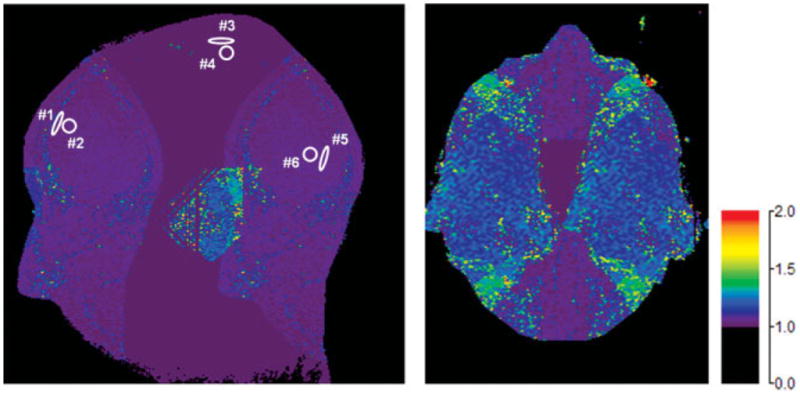
Images of g-factors for R = 4 2D SENSE whole-brain acquisitions taken from midline sagittal (a) and midbrain axial (b) sections. The color scale quantitates the g-values. Measured g-values for ROIs 1– 6 identified in a are tabulated in Table 1 and are representative of those used for measurements of rSNR.

Table 1.

Summary of Measured g-Factors for Regions of Interest Within the Superior Sagittal Sinus

	Anterior		Superior		Posterior
	Vessel	Bkgd	Vessel	Bkgd	Vessel	Bkgd
ROI identifier in Fig. 3a	#1	#2	#3	#4	#5	#6
Area of ROI (mm2)	20.8	45.2	22.6	48.8	48.8	48.8
Area of ROI (number of pixels)	34	74	37	80	80	80
Range of g-values	1.02–1.05	1.01–1.06	1.00–1.00	1.00–1.00	1.02–1.05	1.02–1.06
Mean g-value	1.03	1.03	1.00	1.00	1.04	1.03
SD	0.01	0.01	0.00	0.00	0.01	0.01
g-value used for calculating Aexp	1.03		1.00		1.04
Mean g-value within region across all 20 volunteers	1.031 ± 0.016		1.000 ± 0.000		1.042 ± 0.022
Standard deviation of g-value within region across all 20 volunteers	0.023 ± 0.018		0.000 ± 0.000		0.022 ± 0.020

Bkgd = background, Aexp = signal amplification.

Effects of Tissue Inhomogeneity

In nonaccelerated MRI, it is common when measuring the SNR to take as the noise level the SD in the reconstructed values in air, outside the object, along the phase-encoding direction (28). However, in SENSE-accelerated images, regions outside the object are generally not reconstructed because of a lack of calibration information, and these areas are masked out in the display. Thus, if one attempts to use measurements within the object, even if such measurements are confined to small areas in which the g-factor is only slowly varying, they are still prone to effects caused by any underlying inhomogeneity in the object, as opposed to the statistical noise level.

For the specific hypothesis under study in this work—the existence of an intrinsic amplification of the vascular SNR—tissue inhomogeneity can mimic this effect. This can be understood as follows: Suppose the SD of the statistical noise in a small region of background tissue in an unaccelerated image is σ_N. Also suppose that the SD of the underlying nonhomogeneous tissue signal in the same region is σ_t. Then, the observed SD in a measurement of the reconstructed values in that region will be a combination of the statistical and inhomogeneous components. If the measured signal level for that region is S, and if it is assumed that the two components of the SD add in quadrature, then the observed SNR is given by:

$$\text{SNR}=\frac{\text{S}}{{[{\sigma }_{\text{N}}^2+{\sigma }_1^2]}^{1/2}}$$ [9]

Next, suppose that a SENSE-accelerated acquisition is performed. If the object magnetization is constant over the acquisition, the mean SENSE signal will match the mean signal in the unaccelerated scan. Also, the tissue inhomogeneity levels in both scans will match. However, the statistical noise level will increase in accordance with the standard SENSE behavior. In this case the SNR of the SENSE scan will be:

$$\text{SNR}=\frac{\text{S}}{{[{\sigma }_{\text{t}}^2+\text{R}·{\text{g}}^2·{\sigma }_{\text{N}}^2]}^{1/2}}$$ [10]

The rSNR in background tissue can be defined as the ratio of Eq. [10] to Eq. [9]:

$${\text{rSNR}}_{\text{t}}=\frac{{[{\sigma }_{\text{t}}^2+{\sigma }_{\text{N}}^2]}^{1/2}}{{[{\sigma }_{\text{t}}^2+\text{R}·{\text{g}}^2·{\sigma }_{\text{N}}^2]}^{1/2}}$$ [11]

If the tissue inhomogeneity is parameterized in terms of the statistical noise level, i.e.,

$${\sigma }_{\text{t}}=\alpha ·{\sigma }_{\text{N}}$$ [12]

then rSNR_t can be reexpressed as:

$${\text{rSNR}}_1=\frac{1}{\text{g}·\sqrt{\text{R}}}·{\left[\frac{(1+{\alpha }^2)}{\left(1+\frac{{\alpha }^2}{{\text{g}}^2·\text{R}}\right)}\right]}^{1/2}$$ [13]

This reverts to the standard SENSE equation if there is no contribution to the measured noise level from tissue inhomogeneity, i.e., α = 0. However, for any nonzero tissue inhomogeneity the quantity within brackets exceeds unity and the rSNR is larger than that predicted by the SENSE equation, and as a consequence mimics the very effect being studied in this work. Thus, it is important to somehow distinguish SNR amplification due to modulation of the vascular signal from that intrinsic to taking measurements within non-enhancing tissue.

Evaluation

The hypothesis was tested by comparing the rSNR in enhancing vasculature with that in adjacent nonvascular background tissue. The vascular signal was measured as the mean of a 20–50 mm² ROI within the anterior aspect of the SSS in a central sagittal partition (e.g., ROI 1 of Fig. 3). The noise was taken as the SD in nonvascular, low-signal brain tissue in a similarly-sized ROI located no further than 2 cm from the SSS ROI in the same partition (ROI 2). Such regions are also illustrated in Fig. 4a. The SNR was taken to be the ratio of the signal to the noise measures just described. This process was performed for both the SENSE and non-SENSE scans. The experimental rSNR, rSNR_exp, was then calculated from the ratio:

$${\text{rSNR}}_{\mathit{exp}}=\frac{{\text{SNR}}_{\text{SENSE}}}{{\text{SNR}}_{\text{Non}-\text{SENSE}}}$$ [14]

FIG. 4.

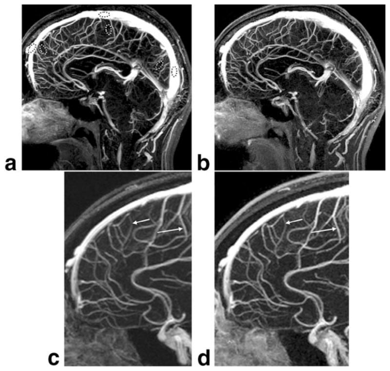
Comparison of midline sagittal partitions taken from reference non-SENSE (a) and R = 4 SENSE (b) whole-brain MR venograms from volunteer 7. Enlargements c and d, which correspond to the dashed box regions of a and b, respectively, illustrate improved vessel sharpness of the SENSE result (arrows, d vs. c) for equal sampling resolution. In this volunteer the SENSE acquisition was done with the second bolus injection. The window and level are normalized to the vessel signal and background.

Using Eq. [8] and the mean measured g-value of 1.03 for the anterior portion of the SSS (Table 1), the experimentally measured amplification factor A_exp was then calculated as:

$${\text{A}}_{exp}={\text{rSNR}}_{exp}\text{g}\sqrt{\text{R}}$$ [15]

The above process was then repeated for background tissue. In this case the mean value within ROI 2 was taken as the signal level, the SD within ROI 2 was used as the noise measure, and the ratio was taken to determine the SNR. This was done for the SENSE and non-SENSE scans, and rSNR_exp and A_exp were calculated for background tissue per Eqs. [14] and [15], and compared with the corresponding values for the vasculature. Because the noise is taken from ROI 2 for both the vascular and background measurements, both are subject to the identical g-factor and the identical effect of tissue inhomogeneity.

The process was repeated for all 20 volunteer studies. Mean values of rSNR_exp and A_exp were calculated separately for the 10 volunteers in whom the non-SENSE scan was done using the first contrast injection, and the other 10 volunteers in whom SENSE was performed using the first injection as well as in aggregate. This was done to check for any potential bias from residual contrast from the first vs. second injection even with the 10-min delay between scans. The hypothesis was tested by determining whether the mean value of A_exp was larger for the vasculature than for the background tissue. Significance was tested by means of a one-tailed Student’s t-test using paired samples (29), with P < 0.05 taken as significant.

This process was repeated for regions in the superior and posterior aspects of the SSS using the respective mean g-values of 1.00 and 1.04 (Table 1). If necessary, in some volunteers a sagittal partition different from that used for the anterior aspect of the SSS was used for the superior or posterior aspects to account for any slight obliquity of the head orientation, but in all cases the signal and noise were measured from the same partition. Also, because of large potential inaccuracy of very low SNR values due to signal rectification (30), any sample for which one of the measured SNR values was less than 2 was discarded from the statistical analysis, with the number of degrees of freedom reduced accordingly.

RESULTS

The measured results for rSNR_exp and A_exp are summarized in Table 2. The range in the individual values reflects intervolunteer variability. Looking at the cumulative results for rSNR_exp, the results for the vascular regions are significantly larger than for adjacent background tissue for all three regions, with P < 0.01, 0.01, and 0.02, respectively. Because the fractional uncertainty in g (typically <3% per Table 1) is small compared to that in rSNR_exp (typically 0.10/0.55 per Table 2, or 18%), upon conversion of rSNR_exp to A_exp the results are maintained with the same level of precision and significance. Thus, the hypothesis is proven.

Table 2.

Summary of Experimental Relative SNR (rSNRexp) and Signal Amplification (Aexp) Measurements for Background Tissue and Vasculature^*

Volunteer	rSNRexp									Aexp
	Anterior			Superior			Posterior			Anterior			Superior			Posterior
	Bkgd	Vascular	Δ	Bkgd	Vascular	Δ	Bkgd	Vascular	Δ	Bkgd	Vascular	Δ	Bkgd	Vascular	Δ	Bkgd	Vascular	Δ
First injection: non-SENSE (N = 10)
1	0.31	0.52	0.22	0.81	0.69	−0.12				0.63	1.07	0.44	1.62	1.38	−0.24
3	0.82	0.91	0.09	0.55	0.67	0.13	0.69	0.59	−0.10	1.70	1.88	0.18	1.09	1.35	0.25	1.44	1.24	−0.21
5	0.63	0.80	0.18	0.44	0.67	0.23	0.40	0.48	0.07	1.29	1.66	0.37	0.89	1.34	0.45	0.84	0.99	0.15
7	0.39	0.44	0.05				0.39	0.34	−0.05	0.80	0.90	0.10				0.81	0.70	−0.11
8	0.42	0.62	0.20	0.61	0.78	0.17	0.51	0.62	0.11	0.88	1.29	0.41	1.22	1.56	0.33	1.06	1.30	0.24
10	0.43	0.68	0.25	0.61	0.52	−0.10	0.42	0.52	0.11	0.88	1.40	0.52	1.23	1.03	−0.20	0.87	1.09	0.22
12	0.39	0.48	0.08	0.47	0.55	0.08	0.49	0.55	0.06	0.81	0.99	0.17	0.94	1.10	0.16	1.03	1.15	0.12
14	0.86	0.81	−0.05	0.52	0.49	−0.04	0.41	0.46	0.06	1.77	1.67	−0.10	1.05	0.97	−0.08	0.84	0.97	0.12
17	0.39	0.56	0.17	0.52	0.59	0.08	0.51	0.61	0.10	0.80	1.15	0.35	1.04	1.19	0.15	1.06	1.27	0.21
19				0.46	0.48	0.02	0.50	0.63	0.13				0.92	0.96	0.04	1.03	1.30	0.27
Mean	0.52	0.65	0.13	0.56	0.60	0.05	0.48	0.53	0.05	1.06	1.33	0.27	1.11	1.21	0.10	1.00	1.11	0.11
SD of mean	0.06	0.05	0.03	0.04	0.03	0.04	0.03	0.03	0.03	0.13	0.11	0.07	0.07	0.07	0.08	0.06	0.06	0.05
t-value			4.15			1.23			2.08			4.15			1.23			2.08
P-value			<0.01			NS			<0.05			<0.01			NS			<0.05
First injection: SENSE (N = 10)
2	0.58	0.62	0.04	0.48	0.66	0.18	0.39	0.63	0.24	1.19	1.28	0.09	0.96	1.32	0.36	0.82	1.32	0.50
4	0.55	0.56	0.01	0.38	0.52	0.14	0.71	0.64	−0.08	1.13	1.16	0.03	0.76	1.04	0.27	1.49	1.32	−0.16
6	0.61	0.63	0.02	0.50	0.61	0.11	0.68	0.69	0.01	1.26	1.29	0.03	1.00	1.22	0.22	1.41	1.43	0.02
9	0.33	0.57	0.24	0.35	0.86	0.51	0.39	0.71	0.32	0.68	1.17	0.49	0.70	1.72	1.03	0.81	1.48	0.67
11	0.48	0.57	0.08	0.64	0.77	0.13	0.51	0.66	0.15	0.99	1.17	0.17	1.28	1.55	0.27	1.06	1.38	0.32
13	0.60	0.46	−0.14	0.58	0.84	0.26	0.70	0.77	0.07	1.24	0.95	−0.29	1.15	1.67	0.52	1.46	1.61	0.15
15	0.53	0.50	−0.03	0.58	0.85	0.27	0.49	0.48	−0.01	1.09	1.03	−0.06	1.17	1.70	0.53	1.03	1.01	−0.02
16	0.42	0.53	0.11	0.52	0.66	0.14	0.41	0.42	0.01	0.87	1.09	0.22	1.04	1.32	0.27	0.84	0.87	0.02
18	0.54	0.53	−0.02	0.57	0.70	0.13	0.51	0.49	−0.02	1.12	1.08	−0.03	1.13	1.40	0.26	1.06	1.02	−0.04
20	0.65	0.70	0.05	0.74	0.79	0.05	0.48	0.42	−0.06	1.33	1.44	0.11	1.48	1.58	0.10	1.01	0.88	−0.12
Mean	0.53	0.57	0.04	0.53	0.73	0.19	0.53	0.59	0.06	1.09	1.17	0.08	1.07	1.45	0.38	1.10	1.23	0.13
SD of mean	0.03	0.02	0.03	0.04	0.04	0.04	0.04	0.04	0.04	0.06	0.04	0.06	0.07	0.07	0.08	0.08	0.08	0.09
t-value			1.18			4.66			1.52			1.18			4.66			1.52
P-value			NS			<0.01			NS			NS			<0.01			NS
Cumulative results (N = 20)
Mean	0.52	0.60	0.08	0.54	0.67	0.12	0.51	0.57	0.06	1.08	1.25	0.17	1.09	1.34	0.25	1.05	1.18	0.12
SD of mean	0.03	0.03	0.02	0.03	0.03	0.03	0.03	0.03	0.02	0.07	0.06	0.05	0.05	0.06	0.07	0.05	0.05	0.05
t-value			3.35			3.81			2.41			3.35			3.81			2.41
P-value			<0.01			<0.01			<0.02			<0.01			<0.01			<0.02

^*For both Rexp and Aexp, Δ is defined as the difference between the vascular and background values immediately to the left. The blank entries are for cases in which results were discarded because the raw SNR values were <2 and prone to high inaccuracy. Mean g-factors used for Regions 1, 2, and 3, are 1.03, 1.00, and 1.04, respectively (Table 1). Regions used are from the anterior, superior, and posterior portions of superior sagittal sinus.

Bkgd = background, NS = not significant.

For the non-SENSE-first group the mean values of rSNR-_exp and A_exp for the vasculature in the anterior and posterior regions are significantly larger than for the background tissue, with P < 0.01 and 0.05, respectively. For the other region (superior), the values for the vasculature are larger than for the background tissue but are not significant (P > 0.05). For the SENSE-first group, the rSNR_exp and A_exp are larger for vasculature vs. background for all three regions, but are statistically significant only for the superior region.

Although not shown in Table 2, when the results from the non-SENSE-first studies are pooled from the three vascular regions (30 samples less three discards), the rSNR and A_exp are larger for vasculature vs. background with P < 0.01. Similarly, when the SENSE-first studies are pooled (30 samples), the same result is obtained with the same significance. These results indicate that there is no bias in whether the SENSE scan was first or second.

Figure 4 is a sample comparison of the midline sagittal partition from a reference non-SENSE acquisition (a) and R = 4 2D SENSE result (b) from volunteer 7. In this volunteer the SENSE scan was done using the second contrast injection. Note the comparable image quality between Fig. 4a and b, especially around the superior portions of the brain where the SNR measurements were made, and where the g-factor values are known from Fig. 3 to be near unity.

DISCUSSION

It has been shown how the application of the 2D SENSE parallel acquisition technique to EC-encoded CE-MRA and MRV can provide a signal amplification A. This can compensate in part for the loss in SNR of $g\sqrt{\text{R}}$ in SENSE scans due to the reduced number of samples and the coil g-factor. The signal amplification is due to the scaling in k-space caused by SENSE of a transient magnetization level that is forced to decrease monotonically in the k_Y-k_Z plane by the EC phase-encoding order. The theoretical bound on the amplification factor A is R = R_Y × R_Z, which occurs when the magnetization has substantially decayed to zero over the duration of the non-SENSE scan. This signal amplification effect was derived analytically, shown graphically, predicted numerically, and demonstrated experimentally in 2D SENSE whole-brain MR venograms with acceleration of R = 4. The mean experimental measurements of A_exp from three specific regions over 20 volunteer studies all exceeded those of adjacent background tissue, which themselves exceeded unity.

A potential complicating factor in using measurements of the noise level from within the nonzero background tissue is the inhomogeneity in this tissue signal. As shown in Eqs. [11]–[13], the variation in this background signal can itself cause the rSNR of the SENSE-to-unaccelerated scans to be larger than that expected using the standard SENSE noise behavior, leading to an A_exp that artifactually exceeds unity and mimics the very effect under study. The hypothesis of this work was demonstrated by showing that the A_exp of the enhancing vasculature was larger than even that of the surrounding background tissue. This was proven using no assumption or measurement of the parameter α of Eq. [12]. Rather, the ROI sizes used were small enough that the tissue inhomogeneity effect was not significant but still large enough to provide adequate statistical power over the set of volunteer studies.

An additional potential complicating factor is the spatial variation of the g-factor. For a given acceleration R, in general this is known to be less severe in 2D vs. 1D SENSE (18). The smooth behavior of the g-map within the typical sagittal partition used can be appreciated from Fig. 3a. For this work, small ROIs were selected in which the variation in g-values was small (3% or less). Moreover, these g-values and g-value maps in general were highly consistent across all 20 volunteers, primarily due to the consistent intersubject position of the SSS within the FOV.

Yet another possible complication is the rectification of signal and noise under conditions of low SNR (30). Each measurement of rSNR was formed from the ratio of two SNR values (one from a non-SENSE image and the other from a SENSE image). Under low-SNR conditions the magnitude operation causes the measured SNR to overestimate the actual SNR. However, other than discarding several samples, no correction was deemed necessary. Within the vascular regions all 120 SNR values exceeded 18 and rectification effects were insignificant. For the nonvascular background tissue, all 60 measured SNR values in the non-SENSE image exceeded 3.5 and the overestimation was small, on the order of several percent. In the SENSE images the measured SNR of background tissue was in all 60 instances smaller than in the companion non-SENSE measurement, and thus the degree of overestimation was larger. This means that any corrected rSNR value in background tissue would be smaller than that measured, thereby increasing the difference with the rSNR of the vasculature. To avoid high potential inaccuracy, for the three instances in which the measured SNR of background in the SENSE image was less than 2, the data were eliminated from analysis (reflected as blank entries in Table 2). Retaining or correcting these low-SNR data would have increased the t-values and further strengthened the statistical significance. It is noted that the minimum SNR of tissue inhomogeneity superimposed on a mean signal can upon rectification have a minimum value smaller than the 1.91 value of Ref. 30 because the inhomogeneity is solely along the real channel.

The observed values of A_exp for the aggregate 20 cases were 1.24, 1.31, and 1.26 for the three regions. Normalizing these values to those observed in the adjacent tissue, the degrees of signal amplification due to the effect under study are calculated as 1.17, 1.24, and 1.21 for the three regions, which compare favorably with the factor of 1.31 determined from Fig. 2.

In a separate experiment, the parameter α of Eq. [12] was estimated. Two unaccelerated image sets from a volunteer were formed using the same 3D image acquisition technique as described above. The volunteer was asked to keep as immobile as possible, the image sets were formed with minimal time delay between them, and no contrast agent was used. A central sagittal partition similar to that used for the above-described analysis was taken from each un-subtracted image set and the difference between them was formed. ROIs similar to those used previously were identified and the SDs were measured in the difference and unsubtracted images and taken respectively to be estimates for ${\sigma }_{\text{N}}\sqrt{\text{2}}$ and ${[{\sigma }_{\text{N}}^2+{\alpha }^2·{\sigma }_{\text{N}}^2]}^{1/2}$, i.e., the deterministic tissue inhomogeneity was assumed to subtract out in the difference image. From these estimates, α was estimated to be approximately 0.3, which when inserted into Eq. [13] leads to an intrinsic amplification factor A of 1.07 from tissue inhomogeneity alone. This compares favorably with the mean values of A_exp for background tissue (1.06, 1.06, and 1.04) in Table 2.

The signal amplification effect in the vasculature described in this work is potentially significant in that higher acceleration factors may be found to be more clinically acceptable for imaging transient magnetization (e.g., contrast-agent passage) than constant magnetization, in which case this effect reverts to A = 1. For example, in this work the mean cumulative rSNR_exp in the vasculature ranged from 0.57 to 0.67 for the fourfold-accelerated SENSE. These values were all larger than the expected rSNR of 0.48 – 0.50 for imaging constant magnetization using our own measured g-factors. In contrast to these results, in the initial 2D SENSE work Weiger et al. (18) measured rSNRs in the range of 0.22– 0.41 (reciprocals of the reported values of 2.4 – 4.4) for much the same kind of pulse sequence (R = 4 GRE imaging of the whole brain) but one with constant magnetization levels and thus no signal amplification effect.

The hypothesis was tested by performing non-SENSE and SENSE CE-MRV in 20 consecutive volunteers. For each volunteer a 10-min wait was used between scans to allow contrast clearance. Although contrast material may persist longer than this (up to several tens of minutes), this is highly subject-specific and it was impractical to wait until residual vessel contrast was reduced to zero from the first scan before performing the second. To account for this, the rSNR_exp and A_exp measurements were made separately for the non-SENSE-scan-first and SENSE-scan-first groups. Because of the reduced statistical power due to having only 10 samples within each group vs. the full 20, in only three of the six cases (two groups × three regions) were the mean A_exp values significantly greater for vessel than for background tissue. However, there was no consistent trend that A_exp was higher for one group vs. the other. Some statistical spread of rSNR_exp and A_exp values, as shown in Table 2, is expected, as has been observed in intersubject tabulations of contrast bolus arrival times in CE-MRA (31).

Related to the signal amplification provided by SENSE imaging of transient magnetization is the potential improvement in net spatial resolution. Figure 4c and d show enlargements of the rectangular dashed regions shown in Fig. 4a and b, respectively, and illustrate improved vessel sharpness in the SENSE result (d) vs. the reference (c). This improvement is due to the PSF of the SENSE-accelerated scan (Eq. [6]) having a narrower width compared to the nonaccelerated case, again a consequence of the signal being maintained at a relatively high level over a broader region of k-space in the accelerated vs. the nonaccelerated case (e.g., Fig. 1b). This effect in which resolution is not dictated solely by sampling was previously demonstrated for 1D parallel imaging (16,17), similarly noted for 1D SENSE CE-MRA (11), and described for non-parallel MR acquisition methods involving nonconstant magnetization, including echo-planar imaging (EPI) (32), fast-spin-echo (FSE) imaging (33), and CE-MRA (19). This result of improved net resolution for the same extent of k-space sampling of 2D SENSE vs. reference is presented here anecdotally. A rigorous study of this effect is outside the scope of this work.

This work used non-time-resolved CE-MRA and MRV with the EC view order as the targeted application for the signal amplification effect. The effect is dependent upon the manner in which the acquisition maps the time-varying signal to k-space, and how this is further altered by the incorporation of SENSE encoding, i.e., the process used to generate Figs. 1 and 2. This phenomenon is applicable to other view orders in which, after an initial phase, the long-term behavior is used to map time to increase radial k-space (34). For non-view-shared time-resolved sequences (e.g., Ref. 35), which are simply replications of a non-time-resolved sequence, then depending upon the view order and the timing of the contrast peak with sampling of central k-space, the analysis may apply directly. Other sequences, such as those that use view sharing (e.g., Refs. 36 –39), all need to be considered with respect to their individual sampling pattern. However, in general it is expected that the image formed at peak contrast with a view-shared, SENSE-accelerated sequence will benefit from some degree of the signal amplification effect presented here because the high contrast signal will be extended over a larger extent of k-space due to the increased k-space sampling rate (the effect of Eq. [4]) provided by SENSE.

In summary, it has been shown that the combination of 2D SENSE acceleration and EC phase-encode ordering causes the decreasing magnetization levels in 3D CE-MRA to have less k-space modulation compared to the nonaccelerated case. This provides an intrinsic signal amplification effect that compensates in part for the SNR loss in SENSE due to the traditional factor $g\sqrt{\text{R}}$.

References

- 1.Pruessmann KP, Weiger M, Scheidegger MB, Boesiger P. SENSE: sensitivity encoding for fast MRI. Magn Reson Med. 1999;42:952–962. [PubMed] [Google Scholar]
- 2.Sodickson DK, Manning WJ. Simultaneous acquisition of spatial harmonics (SMASH): fast imaging with radiofrequency coil arrays. Magn Reson Med. 1997;38:591–603. doi: 10.1002/mrm.1910380414. [DOI] [PubMed] [Google Scholar]
- 3.Griswold MA, Jakob PM, Heidemann RM, Nittka M, Jellus V, Wang J, Kiefer B, Haase A. Generalized autocalibrating partially parallel acquisitions (GRAPPA) Magn Reson Med. 2002;47:1202–1210. doi: 10.1002/mrm.10171. [DOI] [PubMed] [Google Scholar]
- 4.Ohliger MA, Grant AK, Sodickson DK. Ultimate intrinsic signal-to-noise ratio for parallel MRI: electromagnetic field considerations. Magn Reson Med. 2003;50:1018–1030. doi: 10.1002/mrm.10597. [DOI] [PubMed] [Google Scholar]
- 5.Wiesinger F, Boesiger P, Pruessmann KP. Electrodynamics and ultimate SNR in parallel MR imaging. Magn Reson Med. 2004;52:376–390. doi: 10.1002/mrm.20183. [DOI] [PubMed] [Google Scholar]
- 6.Weiger M, Pruessman KP, Kassner A, Roditi G, Lawton T, Ried A, Boesinger P. Contrast-enhanced 3D MRA using SENSE. J Magn Reson Imaging. 2000;12:671–677. doi: 10.1002/1522-2586(200011)12:5<671::aid-jmri3>3.0.co;2-f. [DOI] [PubMed] [Google Scholar]
- 7.Golay X, Brown SJ, Itoh R, Melhem ER. Time-resolved contrast-enhanced carotid MR angiography using sensitivity encoding (SENSE) AJNR Am J Neuroradiol. 2001;22:1615–1619. [PMC free article] [PubMed] [Google Scholar]
- 8.Maki JH, Wilson GJ, Eubank WB, Hoogeveen RM. Utilizing SENSE to achieve lower station sub-millimeter isotropic resolution and minimal venous enhancement in peripheral MR angiography. J Magn Reson Imaging. 2002;15:484–491. doi: 10.1002/jmri.10079. [DOI] [PubMed] [Google Scholar]
- 9.Ohno Y, Kawamitsu H, Higashino T, Takenaka D, Watanabe H, Van Cauteren M, Fuji M, Hatabu H, Sugimura K. Time-resolved contrast-enhanced pulmonary MR angiography using sensitivity encoding (SENSE) J Magn Reson Imaging. 2003;17:330–336. doi: 10.1002/jmri.10261. [DOI] [PubMed] [Google Scholar]
- 10.deVries M, Nijenhuis RJ, Hoogeveen RM, de Haan MW, van Engelshoven JM, Leiner T. Contrast-enhanced peripheral MR angiography using SENSE in multiple stations: feasibility study. J Magn Reson Imaging. 2005;21:37–45. doi: 10.1002/jmri.20240. [DOI] [PubMed] [Google Scholar]
- 11.Born M, Willinek WA, Gieseke J, von Falkenhausen M, Schild H, Kuhl CK. Sensitivity encoding (SENSE) for contrast-enhanced 3D MR angiography of the abdominal arteries. J Magn Reson Imaging. 2005;22:559–565. doi: 10.1002/jmri.20425. [DOI] [PubMed] [Google Scholar]
- 12.Riedy G, Golay X, Melhem ER. Three-dimensional isotropic contrast-enhanced MR angiography of the carotid artery using sensitivity-encoding and random elliptic centric k-space filling: technique optimization. Neuroradiology. 2005;47:668–673. doi: 10.1007/s00234-005-1416-2. [DOI] [PubMed] [Google Scholar]
- 13.Kramer H, Schoenberg SO, Nikolaou K, Huber A, Struwe A, Winnik E, Wintersperger BJ, Dietrich O, Kiefer B, Reiser MF. Cardiovascular screening with parallel imaging techniques and a whole-body MR imager. Radiology. 2005;236:300–310. doi: 10.1148/radiol.2361040609. [DOI] [PubMed] [Google Scholar]
- 14.Wilman AH, Riederer SJ. Performance of an elliptical centric view order for signal enhancement and motion artifact suppression in breathhold three dimensional gradient echo imaging. Magn Reson Med. 1997;38:793–802. doi: 10.1002/mrm.1910380516. [DOI] [PubMed] [Google Scholar]
- 15.Wilman AH, Riederer SJ, King BF, Debbins JP, Rossman PJ, Ehman RL. Fluoroscopically-triggered contrast-enhanced three-dimensional MR angiography with elliptical centric view order: application to the renal arteries. Radiology. 1997;205:137–146. doi: 10.1148/radiology.205.1.9314975. [DOI] [PubMed] [Google Scholar]
- 16.Griswold MA, Jakob PM, Chen Q, Goldfarb JW, Manning WJ, Edelman RR, Sodickson DK. Resolution enhancement in single-shot imaging using simultaneous acquisition of spatial harmonics (SMASH) Magn Reson Med. 1999;41:1236–1245. doi: 10.1002/(sici)1522-2594(199906)41:6<1236::aid-mrm21>3.0.co;2-t. [DOI] [PubMed] [Google Scholar]
- 17.Jaermann T, Pruessman KP, Valavanis A, Kollias S, Boesinger P. Influence of SENSE on image properties in high-resolution single-shot echo-planar DTI. Magn Reson Med. 2006;55:335–342. doi: 10.1002/mrm.20769. [DOI] [PubMed] [Google Scholar]
- 18.Weiger M, Pruessman KP, Boesinger P. 2D SENSE for faster 3D MRI. Magma. 2002;14:10–19. doi: 10.1007/BF02668182. [DOI] [PubMed] [Google Scholar]
- 19.Fain SB, Riederer SJ, Bernstein MA, Huston J. Theoretical limits of spatial resolution in elliptical-centric contrast-enhanced 3D-MRA. Magn Reson Med. 1999;42:1106–1116. doi: 10.1002/(sici)1522-2594(199912)42:6<1106::aid-mrm15>3.0.co;2-q. [DOI] [PubMed] [Google Scholar]
- 20.Thompson HK, Starmer F, Whalen RE, McIntosh HD. Indicator transit time considered as a gamma variate. Circ Res. 1964;14:502–515. doi: 10.1161/01.res.14.6.502. [DOI] [PubMed] [Google Scholar]
- 21.Haacke EM, Brown RW, Thompson MR, Venkatesan R. Magnetic resonance imaging: physical principles and sequence design. New York: Wiley-Liss; 1999. pp. 269–272. [Google Scholar]
- 22.Haider CR, Hu HH, Madhuranthakam AJ, Kruger DG, Campeau NG, Huston J, III, Riederer SJ. Time-resolved 3D contrast-enhanced MRA with 2D homodyne and view sharing for contrast bolus dynamics of the brain. Proceedings of the 14th Annual Meeting of ISMRM; Seattle, WA, USA. 2006. p. Abstract 812. [Google Scholar]
- 23.Fain SB, Riederer SJ. Dependence of venous enhancement on the field of view in 3D contrast-enhanced MRA using the elliptical centric view order. Magn Reson Med. 2001;45:1134–1141. doi: 10.1002/mrm.1151. [DOI] [PubMed] [Google Scholar]
- 24.Farb RI, Scott JN, Willinsky RA, Wright GA, terBrugge KG. Intracranial venous system: gadolinium-enhanced three-dimensional MR venography with auto-triggered elliptic centric-ordered sequence—initial experience. Radiology. 2003;226:203–209. doi: 10.1148/radiol.2261020670. [DOI] [PubMed] [Google Scholar]
- 25.Wetzel SG, Law M, Lee VS, Cha S, Johnson GA, Nelson K. Imaging of the intracranial venous system with a contrast-enhanced volumetric interpolated examination. Eur Radiol. 2003;13:1010–1018. doi: 10.1007/s00330-002-1714-6. [DOI] [PubMed] [Google Scholar]
- 26.Mermuys KP, Vanhoenacker PK, Chappel P, Van Hoe L. Three-dimensional venography of the brain with a volumetric interpolated sequence. Radiology. 2005;234:901–908. doi: 10.1148/radiol.2343031956. [DOI] [PubMed] [Google Scholar]
- 27.Nael K, Fenchel M, Salamon N, Duckwiler GR, Laub G, Finn JP, Villablanca JP. Three-dimensional cerebral contrast-enhanced magnetic resonance venography at 3. 0 Tesla. Invest Radiol. 2006;41:763–768. doi: 10.1097/01.rli.0000236992.21065.04. [DOI] [PubMed] [Google Scholar]
- 28.Haacke EM, Brown RW, Thompson MR, Venkatesan R. Magnetic resonance imaging: physical principles and sequence design. New York: Wiley-Liss; 1999. p. 340. [Google Scholar]
- 29.Rosner B. Fundamentals of biostatistics. Duxbury Press; Belmont CA: Thomson Learning; 2000. pp. 275–278. [Google Scholar]
- 30.Henkelman RM. Measurement of signal intensities in the presence of noise in MR images. Med Phys. 1985;12:232–233. doi: 10.1118/1.595711. [DOI] [PubMed] [Google Scholar]
- 31.Riederer SJ, Bernstein MA, Breen JF, Busse RF, Ehman RL, Fain SB, Hulshizer TC, Huston J, King BF, Kruger DG, Shah S. Three-dimensional contrast-enhanced MR angiography with real-time fluoroscopic triggering: design specifications and technical reliability in 330 patient studies. Radiology. 2000;215:584–593. doi: 10.1148/radiology.215.2.r00ma21584. [DOI] [PubMed] [Google Scholar]
- 32.Farzaneh F, Riederer SJ, Pelc NJ. Analysis of T2 limitations and off-resonance effects on spatial resolution and artifacts in echo-planar imaging. Magn Reson Med. 1990;14:123–139. doi: 10.1002/mrm.1910140112. [DOI] [PubMed] [Google Scholar]
- 33.Constable RT, Gore JC. The loss of small objects in variable TE imaging: implications for FSE, RARE, and EPI. Magn Reson Med. 1992;28:9–24. doi: 10.1002/mrm.1910280103. [DOI] [PubMed] [Google Scholar]
- 34.Willinek WA, Gieseke J, Conrad R, Strunk H, Hoogeveen R, von Falkenhausen M, Keller E, Urbach H, Kuhl CK, Schild HH. Randomly segmented central k-space ordering in high-spatial-resolution contrast-enhanced MR angiography of the supraaortic arteries: initial experience. Radiology. 2002;225:583–588. doi: 10.1148/radiol.2252011167. [DOI] [PubMed] [Google Scholar]
- 35.Finn JP, Baskaran V, Carr JC, McCarthy RM, Pereles FS, Kroeker R, Laub G. Thorax: low-dose contrast-enhanced three-dimensional MR angiography with subsecond temporal resolution—initial results. Radiology. 2002;224:896–904. doi: 10.1148/radiol.2243010984. [DOI] [PubMed] [Google Scholar]
- 36.Riederer SJ, Tasciyan T, Farzaneh F, Lee JN, Wright RC, Herfkens RJ. MR fluoroscopy: technical feasibility. Magn Reson Med. 1988;8:1–15. doi: 10.1002/mrm.1910080102. [DOI] [PubMed] [Google Scholar]
- 37.van Vaals JJ, Brummer ME, Dixon WT, Tuithof HH, Engels H, Nelson RC, Gerety BM, Chezmar JL, denBoer JA. “Keyhole” method for accelerating imaging of contrast agent uptake. J Magn Reson Imaging. 1993;3:671–675. doi: 10.1002/jmri.1880030419. [DOI] [PubMed] [Google Scholar]
- 38.Korosec FR, Frayne R, Grist TM, Mistretta CA. Time-resolved contrast-enhanced 3D MR angiography. Magn Reson Med. 1996;36:345–351. doi: 10.1002/mrm.1910360304. [DOI] [PubMed] [Google Scholar]
- 39.Cashen TA, Carr JC, Shin W, Walker MT, Futterer SF, Shaibani A, McCarthy FM, Carroll TJ. Intracranial time-resolved contrast-enhanced MR angiography at 3T. AJNR Am J Neuroradiol. 2006;27:822–829. [PMC free article] [PubMed] [Google Scholar]