Recognition of prokaryotic promoters based on a novel variable-window Z-curve method

Abstract

Transcription is the first step in gene expression, and it is the step at which most of the regulation of expression occurs. Although sequenced prokaryotic genomes provide a wealth of information, transcriptional regulatory networks are still poorly understood using the available genomic information, largely because accurate prediction of promoters is difficult. To improve promoter recognition performance, a novel variable-window Z-curve method is developed to extract general features of prokaryotic promoters. The features are used for further classification by the partial least squares technique. To verify the prediction performance, the proposed method is applied to predict promoter fragments of two representative prokaryotic model organisms (Escherichia coli and Bacillus subtilis). Depending on the feature extraction and selection power of the proposed method, the promoter prediction accuracies are improved markedly over most existing approaches: for E. coli, the accuracies are 96.05% (σ⁷⁰ promoters, coding negative samples), 90.44% (σ⁷⁰ promoters, non-coding negative samples), 92.13% (known sigma-factor promoters, coding negative samples), 92.50% (known sigma-factor promoters, non-coding negative samples), respectively; for B. subtilis, the accuracies are 95.83% (known sigma-factor promoters, coding negative samples) and 99.09% (known sigma-factor promoters, non-coding negative samples). Additionally, being a linear technique, the computational simplicity of the proposed method makes it easy to run in a matter of minutes on ordinary personal computers or even laptops. More importantly, there is no need to optimize parameters, so it is very practical for predicting other species promoters without any prior knowledge or prior information of the statistical properties of the samples.

INTRODUCTION

In genetics, a promoter is a region of DNA that facilitates the transcription of particular genes. In bacteria, the promoter is recognized by RNA polymerase (RNAP) and associated sigma factors, which may be recruited to the promoter by regulatory proteins binding to specific sites in the region. Thus, control of transcription initiation accounts for much of the overall regulation of gene expression (1). The continued development of large, sophisticated databases and repositories has made vast amounts of biological data accessible to researchers. Additionally, advances in molecular biology and computational techniques are enabling the systematic investigation of the complex molecular processes underlying biological systems. Many algorithms have been developed for the detection of promoters in prokaryotic genomes. For example, Askary et al. and Rangannan and Bansal developed a promoter prediction algorithm based on the difference in stability between neighbouring upstream and downstream regions in the vicinity of experimentally determined transcription start sites (TSSs) (2,3). Rani and Bapi used n-grams (n = 3) as features for a neural network classifier for promoter prediction in Escherichia coli and achieved 67.75% prediction sensitivity and 86.10% specificity (4). Mann et al. used a hybrid technique combining profile hidden Markov models (HMMs) and artificial neural networks (ANNs) methods with Viterbi scoring optimizations (5). Burden et al. and Bland et al. also used ANNs to improve the promoter prediction accuracy (6,7). Lin and Li developed a hybrid approach (called IPMD) combining position correlation score function and increment of diversity with modified Mahalanobis Discriminant to predict eukaryotic and prokaryotic promoters (8). By applying the IPMD to E. coli and Bacillus subtilis promoter sequences, they achieved the sensitivities and specificities of 84.9% and 91.4% for E. coli, as well as 80.4% and 91.3% for B. subtilis.

Although these attempts, which employ sophisticated machine-learning methods to identify promoters, offer increased accuracy in certain circumstances, the improvements may not justify the heavy computational requirements they impose for training classifiers. Moreover, the selection and optimization of parameters (such as the type and parameters of kernel functions, number of hidden layer nodes, etc.) need enough prior knowledge of the statistical properties of the samples, which makes it unpractical for the analysis of new genome sequences.

The regular Z-curve (or Z-curve) method originally proposed by Zhang is a powerful tool in visualizing and analysing DNA sequences (9,10). It is a 3D curve or point representation for a DNA sequence in the sense that each can be uniquely reconstructed given the other. The resulting curve has a zigzag shape, hence the name Z-curve. The 3D curve or point of a given DNA sequence is calculated from the frequencies of the four bases occurring in it to evaluate the sequence from three main components: distribution of purine/pyrimidine, distribution of amino/keto and distribution of strong H-bonds/weak H-bonds. Z-curve method has been used in many different areas of genome research, such as replication origin identification (11,12), ab initio gene prediction (13), isochore identification (14), genomic island identification (15) and comparative genomics (16). However, the regular Z-curve method could not able to extract the information of w-nucleotides sequence patterns occurring in DNA sequences, the promoter recognition accuracy based on it is far from satisfactory.

Hence, a novel variable-window Z-curve (vw Z-curve) method is proposed here as a feature-extraction tool for prokaryotic promoter recognition for the first time. The features extracted by it (with window size w = 1, 2, … , 6) are used as the input variables for further classification by a partial least squares (PLS) classifier. Promoter fragments of two prokaryotic model organisms (E. coli and B. subtilis) are used to verify the prediction performance of the proposed method. The feature extraction power of the vw Z-curve method and the iterative feature selection power of the PLS technique make the prediction performance improved markedly over most existing approaches: for E. coli, the accuracies are 96.05% (σ⁷⁰ promoters, coding negative samples), 90.44% (σ⁷⁰ promoters, non-coding negative samples), 92.13% (known sigma-factor promoters, coding negative samples), 92.50% (known sigma-factor promoters, non-coding negative samples), respectively; for B. subtilis, the accuracies are 95.83% (known sigma-factor promoters, coding negative samples) and 99.09% (known sigma-factor promoters, non-coding negative samples). The results are verified relying on a 10-fold cross-validation jackknife test. Moreover, the proposed method is a linear technique, thus its computational simplicity makes it possible to be run on ordinary personal computers or laptops with run times of several minutes. In particular, because there is no need to optimize parameters, this method is very practical for predicting other species promoters without any prior knowledge or prior information of the statistical properties of the samples.

MATERIALS AND METHODS

Databases

The complete genomic sequences of E. coli K-12 and B. subtilis are obtained from NCBI GenBank (17). The positions of experimentally determined TSSs of them are retrieved from RegulonDB version 7.0 (18) and DBTBS (19). Then promoter regions [TSS-60 … TSS+19] (the site of TSS is +1) are taken as the positive examples. The positive sample database of E. coli consists of two kinds of promoter fragments: 576 experimentally confirmed σ⁷⁰ promoters and 825 experimentally confirmed promoters of several known sigma factors (576 σ⁷⁰ promoters, 63 σ³⁸ promoters, 40 σ³⁸ and σ⁷⁰ promoters, 64 σ²⁴ promoters, 4 σ²⁴ and σ⁷⁰ promoters, 9 σ²⁸ promoters, 44 σ³² promoters, 7 σ³² and σ⁷⁰ promoters, 18 σ⁵⁴ promoters). Considering the comparatively small size of experimentally confirmed B. subtilis promoters, all 660 promoters of known sigma factors (e.g. σ⁴³, σ⁵⁴, σ³⁷ and so on) are used as the positive samples of B. subtilis.

As there is no enough experimentally confirmed negative data (i.e. the positions that are confirmed not to be TSS), the risk has to be taken to choose the negative examples randomly from the same chromosome. Approximately, for E. coli K-12, 81% of known TSSs are located in the intergenic non-coding regions and 19% in the coding regions (20). So two kinds of negative examples are prepared:

1. Coding negative examples: fragments extracted from the coding regions (genes). For E. coli, the coding negative sample set contains 836 80-bp fragments extracted from the start of the open reading frames (ORFs) with lengths of 80–380 bp. For B. subtilis, the coding negative sample set contains 665 80-bp fragments extracted from the start of the ORFs with lengths of 80–335 bp.

2. Non-coding negative examples: fragments extracted from the non-coding regions (convergent intergenic spacers). For E. coli, the non-coding negative sample set contains 825 fragments with lengths of 80 bp. For B. subtilis, the non-coding negative sample set contains 331 fragments with lengths of 80 bp.

The data sets and the corresponding detailed descriptions are shown in Table 1.

Table 1.

The detailed descriptions of data sets

Data set	Positive samples	Negative samples
Data set-1	576 σ70 promoters of E. coli	836 coding fragments of E. coli
Data set-2	576 σ70 promoters of E. coli	825 non-coding fragments of E. coli
Data set-3	825 known sigma-factor promoters of E. coli	836 coding fragments of E. coli
Data set-4	825 known sigma-factor promoters of E. coli	825 non-coding fragments of E. coli
Data set-5	660 known sigma-factor promoters of B. subtilis	665 coding fragments of B. subtilis
Data set-6	660 known sigma-factor promoters of B. subtilis	331 non-coding fragments of B. subtilis

The novel variable-window Z-curve feature extraction method

Being the first transcription step, initiation promoted by interaction of RNAP with gene promoter is a key level of control of gene expression. RNAP holoenzyme is recruited at a given promoter through the recognition of a promoter by transcriptional factors, called ‘sigma (σ) factors’, which are variable subunit of RNAP holoenzyme.

Typically, housekeeping σ⁷⁰ factors of E. coli bind to the −35 and −10 DNA sequence elements in a promoter with the consensus sequences TTGACA at position −35 and TATAAT at position −10, respectively (positions indicate the location of each sequence with respect to the TSS). Two other important sites are the extended −10 element with the consensus sequence ‘TGN’ and the AT-rich UP element (21,22). Alternatively, σ⁵⁴ factors, which control several ancillary processes including the degradation of xylene and toluene, transport of dicarboxylic acids and so on, bind to ‘GG’ at −24 location and ‘GC’ at −12 location of promoters (23). For B. subtilis, DegU promoter has the ‘GNCATTTA’ consensus DNA-binding sequence (24), σ^E-independent sigG promoters have ‘TTT’ and ‘AAA’ motifs (25) and so on.

It is well known that different sigma factors bind to different motifs of promoters. One genome may encode many different σ-factors. In general, bacterial housekeeping sigma-factors, which regulate genes that are involved in cellular growth, σ-factors are similar to the E. coli σ⁷⁰ factors (26,27). Several members of the σ⁷⁰ factor family have been described: E. coli K-12 has six σ⁷⁰ family σ-factors (28), whereas B. subtilis has 17 known variants of σ⁷⁰ (19). A specific subfamily of σ-factors that directly incorporates signals from the extracellular environment in regulating transcription (ECF σ-factors) also exists (29). More details about promoter architecture and sigma factors are available in the Supplementary Data.

Mismatches between RNAP, σ-factors and the given binding sites can be tolerated and even allow for the modulation of promoter strength at some specific genes. Multiple occurrences of promoters in the same regulatory region of one gene can be found for different regulatory functions (30). Unless mutagenesis is performed, each site has the chance to be the place chosen by the RNAP to bind the DNA. Unlike eukaryotic promoters, tightly packed prokaryotic genes and promoters frequently overlap each other (18) obscuring promoter motifs.

Experimental procedures are efficient to identify individual promoters but not conceivable for sets of genes at the whole genome scale. This motivated the search for computational methods based on the knowledge gained about the properties of known promoters or based on an efficient representation of DNA motifs by means of combinatorial or stochastic methods. Unfortunately, the absence of relatively strong sequence patterns identifying true promoters, the diversity of the motifs, the comparatively uncertainty of the locations of the motifs and the incompletely understood mechanisms of the regulation of promoters confound exact predictions of prokaryotic promoters.

The aims of this work are not only to predict promoters with very high accuracy, but to predict promoters of different sigma factors that have different recognition motifs in one collective data set (Tables 1 and 3). So it is important to draw out these distinctions with different sigma factors whose motifs usually comprise more than 1 nt. While the regular Z-curve parameters are only derived from the frequencies of mononucleotides occurring in a DNA sequence. Consequently, the features extracted by regular Z-curve method are not enough for promoter recognition problems and the promoter prediction accuracy based on these features is far from satisfactory. Up to now, only Yang et al. (31) used Z-curve method in Human Pol II promoter recognition.

Table 3.

Prediction results of all known sigma-factor promoters of E. coli using different combination of vw Z-curve features**

Number*	Data set-3					Data set-4
	4095	650	350	280	230	4095	1100	610	360
Results (%)
	79.63	87.07	91.59	91.95	92.44	82.56	89.63	91.34	92.20
	75.98	88.17	90.49	91.46	91.83	84.51	90.12	91.10	92.80
	77.80	87.62	91.04	91.71	92.13	83.54	89.88	91.22	92.50

*Number: number of selected vw Z-curve variables

**The average accuracies of the vw Z-curve methods with 230 parameters for Data set-3 and 360 parameters for Dataset-4, which were the best ones among the algorithms evaluated here, were shown in boldface.

According to the key motifs mentioned above, it is reasonable to assume that the parameters derived from the distributions of w-nucleotides patterns (the window size w∈N) are the essential features which could able to distinguish between promoter regions and non-promoter regions successfully. Hence, a novel variable-window Z-curve (vw Z-curve) method which introduces variable window technique into the regular Z-curve method is developed and used in prokaryotic promoter recognition for the first time to improve the prediction accuracy of the issue. The following paragraphs provide a detailed explanation of the methodology of the vw Z-curve method.

Let Word is a set consisting the 4 nt A, G, C and T, that is: Word = {A,G,C,T}, (the window size w∈N, i = 1, … ,4^w) is a string constructed by picking w elements from the set Word with order and repetition. For example: when w = 2, = ‘AA’, = ‘AT’, = ‘AG’, … , = ‘TT’.

Let the frequency of sequence pattern ‘’ occurring in an ORF or a fragment of DNA sequence be denoted by , where X = A, C, G and T. Using the Z-curve method of DNA sequences (32,33), the uniform definition of vw Z-curve variables (the window size w∈N) could be deduced as Equation (1)

(1)

It can be easily seen that the mono-nucleotide, di-nucleotides and tri-nucleotides phase-independent Z-curve parameters illustrated by Gao and Zhang (32) are the special instances of the vw Z-curve method where w = 1, 2, 3. The detailed descriptions of them are shown in Equations (2–4), respectively.

• (1) The Z curve parameters for frequencies of phase-independent mononucleotides (window size w = 1, variable number n = 3 × 4⁰ = 3): the frequencies of bases A, C, G and T occurring in a DNA sequence are denoted by a, c, g and t, respectively. Based on the Z-curve method, a, c, g and t are mapped onto a point P in a 3D space V, which are denoted by x, y, z (33).

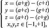(2)

• (2) The Z curve parameters for frequencies of phase-independent di-nucleotides (window size w = 2, variable number n = 3 × 4¹ = 12): let the frequency of di-nucleotides XY be denoted by p(XY), where X, Y = A, C, G and T. Using the Z-curve method of DNA sequences, the following equation could be deduced as:

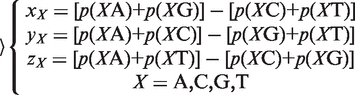(3)

where x_X, y_X and z_X are the coordinates of a point in a 3D space.

• (3) The Z curve parameters for frequencies of phase-independent tri-nucleotides (window size w=3, variable number n = 3 × 4² = 48): using similar notations, it could be deduced as:

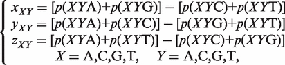(4)

By the same way, the vw Z-curve parameters for frequencies of w-nucleotides could be deduced easily. By a selective combination of n variables or parameters derived from the vw Z-curve method, a DNA sequence can be represented by a point or a vector in an n-dimensional space V.

Unlike the variables extracted by Position Weight Matrix (PWM) based algorithms (30), vw Z-curve parameters are derived from the distributions of w-nucleotides patterns occurring in the same sequence fragment not from their frequencies occurring in different sequence fragments. Thus, the vw Z-curve parameters are not influenced by the uncertainty of motif positions relative to the TSS. Due to the introduce of the window size w, the distributions of w-nucleotides patterns according to different sigma factors could be taken into account synchronously. Consequently, this novel vw Z-curve method is especially suitable for solving motif-finding or pattern recognition (PR) problems of DNA sequence researching.

Considering both the length of those widely known motifs and the computational requirement, the window sizes of the proposed vw Z-curve method used for promoter recognition problems are set w = 1, 2, … ,6. The detailed descriptions of them are shown in Supplementary Table S1.

For researchers’ convenience, the MATLAB codes of the vw Z-curve method are given in the Supplementary Data.

Partial least squares classifier

Supervised pattern analysis could be taken as the regression problems in which the dependent variables are defined as l∈{−1,+1} in two-class problems or as l∈{1, 2, … , N} in multi-class problems, here N is the number of classes. Hence regression algorithms could be used as classifiers in supervised PR.

PLS algorithm is a key technique for modelling linear relationships between a set of output variables (known class-labels) and a set of input variables (predictors). PLS algorithm creates orthogonal latent variables (LVs), which are linear combinations of the original variables. The basic point of the procedure is that the weights used to determine these linear combinations of the original variables are proportional to the maximum covariance among input and output variables (34). Hence, by the projection of the PLS algorithm, the n-dimensional X-space is compressed into the v-dimensional LV-space (v<<n in common cases) to remove the noise and the multi-colinearity of the original data. This leads to a biased but lower variance estimate of the regression coefficients compared to the least squares method (34). PLS has been proven to be very useful in situations where the number of observed variables (n) is significantly greater than the number of observations (m) and high multi-colinearity among the variables exists (35,36). This is especially true in the case of the current study. Thus, PLS is expected to be a useful supervised PR method with potential applications in the discovery of key vw Z-curve features.

For more detailed mathematical descriptions of the PLS classifier, please refer to the Supplementary Data.

The performance of promoter prediction

To evaluate the performance of promoter prediction, the following measurements are used here.

(5)

(6)

(7)

where TP, TN, FP and FN are fractions of positive correct, negative correct, false positive and false negative predictions, respectively.

The sensitivity Sn is the proportion of promoter sequences that have been correctly predicted as promoters. The specificity Sp is the proportion of negative samples that have been correctly predicted as negative samples. The accuracy a is defined as the average of Sn and Sp. Thus the goal in this study is to maximize the prediction accuracy a of testing set as well as make good trade-off between Sn and Sp.

To overcome the randomicity of samples and to evaluate the prediction performance forcefully, 10-fold leave-one-out method is performed as the cross-validation jack-knife test, in which the data set is divided into 10 parts and tested on the 10 different one-tenths while trained on the remaining nine-tenths.

RESULTS AND DISCUSSION

Optimum combination of the vw Z-curve features for promoter prediction using the PLS based iterative feature selection method

Apart from feature extraction, feature selection (also known as variable selection) is one of the most useful techniques for improving the performance of PR. By removing the most irrelevant and redundant features, feature selection helps to do the following:

• Alleviate the effect of the curse of dimensionality.

• Enhance generalizability.

• Speed up the learning process.

• Improve model interpretability.

To select an optimal set of features, it is necessary to quantitatively evaluate the contribution of each feature of the vw Z-curve method. As mentioned above, two-class supervised pattern analysis can be handled as a univariate regression problem in which the dependent variables are defined as l∈{−1,+1}. For univariate regression problems, the absolute value of the regression coefficient of each variable is a reasonable measurement of its contribution.

The total number of all vw Z-curve variables of the issue is 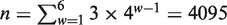(w = 1, … ,6). The absolute values of the coefficients of all 4095 variables in the PLS promoter recognition model of data set-1 and data set-5 are shown in Supplementary Figure S3. The figure shows that only a few variables stand out above the others with high absolute coefficient values. Obviously, important information gets buried in a sea of trivialities, a phenomenon known as ‘information saturation’. Moreover, the methodology of the vw Z-curve method indicates there are strong multi-collinear relationships among all these features. Hence, the feature selection method relying on the PLS algorithm is used to improve the recognition performance.

Considering the large number of variables compared to the number of samples, iterative feature selection is used as a way to improve the recognition performance. The detailed procedure is as follows (take the iterative feature selection of data set-1 for an example):

1. Selecting m positive and m negative samples (here, m = 576, the number of positive samples).

2. Using n vw Z-curve variables for training the promoter recognition model (for first feature selection iteration n = 4095).

3. Sorting variables in descending order according to their absolute coefficient values.

4. Selecting the top p variables (e.g. p = 600) with the highest absolute coefficient values and use of a cross-validation procedure to assess the prediction performance of these selected variables.

5. Optimizing p to maximize the prediction average accuracy and to ensure a good trade-off between sensitivity (Sn) and specificity (Sp) of the recognition model.

6. Repeating steps 2–6 (setting n = p) until the prediction average accuracy converges.

It is notable that, for different sample sets, the iteration number of the feature selection procedure and the optimal combination of vw Z-curve variables may be different.

The prediction results shown in Tables 2–4 demonstrate that the promoter recognition performance strongly lowered by information saturation and multi-collinearity is remarkably improved by the iterative feature selection method.

Table 2.

Prediction results of the σ⁷⁰ promoters of E. coli using different combination of vw Z-curve features**

Number*	Data set-1				Data set-2
	4095	600	350	330	4095	600	500	245	220
Results (%)
	80.00	92.63	95.79	96.32	81.40	88.42	87.02	91.40	92.11
	75.96	93.86	95.61	95.79	75.44	84.74	85.09	86.14	88.77
	77.98	93.25	95.70	96.05	78.42	86.58	86.05	88.77	90.44

*Number: number of selected vw Z-curve variables.

**The average accuracies of the vw Z-curve methods with 330 parameters for Data set-1and 220 parameters for Dataset-2, which were the best ones among the algorithms evaluated here, were shown in boldface.

Table 4.

Prediction results of all known sigma-factor promoters of B. subtilis using different combination of vw Z-curve features**

Number*	Data set-5				Data set-6
	4095	872	405	340	4095	740	490
Results (%)
	80.91	92.73	95.30	95.76	66.97	94.55	98.79
	81.82	91.97	94.24	95.91	73.03	95.76	99.39
	81.36	92.35	94.77	95.83	70.00	95.15	99.09

*Number: number of selected vw Z-curve variables.

**The average accuracies of the vw Z-curve methods with 340 parameters for Data set-5 and 490 parameters for Dataset-6, which were the best ones among the algorithms evaluated here, were shown in boldface.

From the results shown in Table 2, it can be seen that after the first iteration of feature selection, the number of useful vw Z-curve variables is markedly reduced from 4095 variables to 600 variables. By eliminating the interference of irrelevant variables, the prediction accuracy of data set-1 is improved by 15.27%, and the accuracy of data set-2 is improved by 8.16%. These 600 variables are used to build recognition models to again re-evaluate their importance clearly and fairly. To further improve the prediction accuracy, features are selected according to their re-evaluated importance. The prediction accuracy is improved until no more useless variables could be eliminated. After three iterations of feature selection, the final prediction accuracy of data set-1 reaches as high as 96.05%, much better than the accuracy obtained with any previously developed method. The final accuracy of data set-2 is only 90.44%, but it is much better than the accuracy achieved by most other methods. Furthermore, the trade-off between the Sn and Sp is also improved by the feature selection procedure: the difference between Sn and Sp for data set-1 is reduced from 4.04% of 4095 variables to 0.53% of 330 variables; for data set-2, it is reduced from 5.96% to 3.34%.

The prediction results of all experimentally confirmed promoters of known sigma-factors of E. coli are shown in Table 3. It is obvious that the prediction accuracies are both improved markedly using the iterative feature selection method. The highest average accuracies of data set-3 and data set-4 are 92.13% and 92.50%, respectively.

To verify the prediction performance of the proposed method further, it is used to predict promoter sequences of B. subtilis, a typical gram-positive model organism. The samples are contained in data set-5 and data set-6 and the details of them are also shown in Table 1. The prediction results of them are shown in Table 4. Surprisingly, the average accuracies of data set-5 and data set-6 are as high as 95.83% and 99.09% respectively, which are much higher than the accuracies obtained by any other existing method.

Comparison with other existing methods

Evaluation of the performance of the proposed method requires comparisons with other available methods. Because different algorithms use different negative sample sets and different fragment sizes for promoter samples, it is only possible to give a rough comparison between the proposed method and other methods.

Comparing the prediction performance of E. coli promoter

Most existing methods tested their prediction performance using σ⁷⁰ promoter fragments of E. coli K-12 with 80 bp (TSS-60 … TSS+19). They used two kinds of negative samples: coding segments and intergenic segments. The best prediction results of different methods are shown in Table 5 in detail. The most commonly used measurements of these methods are introduced to evaluate the performance of them. For both coding and non-coding negative samples, the performance of the proposed method is much better than that of other methods.

Table 5.

The best prediction results of E. coli promoters obtained by different methods (fragments length is 80 bp)**

Methods	Results (%)
	Sensitivity TP/(TP+FN)	Specificity TN/(TN+FP)	Precision TP/(TP+FP)
Negative samples: Coding segments
IPMD (8)	84.9	91.4	–
Sequence Alignment Kernel+SVM (20)	82	–	84
The proposed method	96.32	95.79	95.81
Negative samples: Intergenic segments
3-gram* (4)	67.75	86.10	–
IPMD (8)	81	92.7	–
Sequence Alignment Kernel+SVM (20)	81	–	81
The proposed method	92.11	88.77	89.13

*The negative sample set contained 709 sequence fragments from the coding region and 709 sequence segments from intergenic portions. Training data set size for E. coli was 1669. The paper did not give more details about the training and testing set.

**The best average accuracies among the algorithms evaluated here were shown in boldface.

When taking intergenic segments as negative samples, the specificity obtained by IPMD is 92.7%, which is higher than the specificity obtained by the proposed method. But the average accuracy (the mean of sensitivity and specificity) obtained by IPMD is 86.85%, while the accuracy obtained by the proposed method is 90.44%. It is obviously, compared with IPMD, the average accuracy is improved by 3.59% by the proposed method. Additionally, the difference between specificity and sensitivity of IPMD and the proposed method is 11.7% and 3.34%, respectively. Consequently, the trade-off between Sn and Sp obtained by the proposed method is much better than that obtained by IPMD.

As mentioned above, approximately, for E. coli K-12, 81% of known TSSs are located in the intergenic non-coding regions and 19% in the coding regions (20). Partly due to these facts, the difference of patterns distribution between coding sequences and promoter sequences is much more statistically significant than that between intergenic sequences and promoter sequences. Consequently, from the results shown in Table 5, it could be seen that, for all listed methods, the recognition performance between promoter and coding sequences is better than that of promoter and non-coding sequences.

The promoter region is less stable and hence more prone to melting as compared to other genomic regions. Thus, there are some methods based on the differences in the stability of DNA sequences in the promoter and non-promoter region. Askary et al. presented a modified ANN (named N4) fed by nearest neighbours and based on DNA duplex stability (2). The promoter prediction sensitivity [TP/(TP+FN)] and precision [TP/(TP+FP)] of N4 for predicting promoters in E. coli are both 94%. To this author’s knowledge, this represents the best result achieved in the existing literature.

Comparisons of the method presented here with that of Askary et al. (2) are made by using the same measurements and similar database construction methods. The positive sample set consists of 576 experimentally confirmed σ⁷⁰ promoters fragments with 414 bp ([−207 … TSS …], the site of TSS is +1). The negative sample set consists of the first 414-bp fragment of the 530 ORFs with length of 414–585 bp. The best recognition results obtained by these two different methods are shown in Table 6. It is also obvious that the prediction accuracy of the proposed method is much better than the accuracy obtained by N4 method.

Table 6.

The best recognition results of E. coli promoters obtained by different methods (fragments length is 414 bp)*

Methods	Sensitivity (%) TP/(TP+FN)	Precision (%) TP/(TP+FP)
The proposed method	97.10	97.31
N4 Neural Networks (2)	94	94

*The best average accuracies among the algorithms evaluated here were shown in boldface.

Comparing the prediction performance of B. subtilis promoter

Bacillus subtilis, a representative Gram positive bacterium, is often used to demonstrate the performance of the prokaryotic promoter prediction methods. Lin and Li applied the IPMD method to predict B. subtilis promoters (8). To this author's knowledge, this represents the best result achieved in the existing literature.

Comparisons of the proposed method with that of Lin and Li (8) are made by using the same measurements and similar database construction methods. The best recognition results obtained by these two different methods are shown in Table 7. In the case of coding negative samples, the prediction average accuracy is improved from 85.85% to 95.83% by the proposed method, as well as the difference between Sn and Sp is decreased from 10.9% to 0.15%. In the case of non-coding negative samples, the prediction average accuracy is improved by 15.54% by the proposed method, as well as the difference between Sn and Sp is decreased by 21.3%. The results strongly indicate that both the prediction accuracy and the trade-off between Sn and Sp are improved remarkably.

Table 7.

The best recognition results of B. subtilis promoters obtained by different methods (fragments length is 80 bp)*

Methods	Results (%)
	Sensitivity (Sn) TP/(TP+FN)	Specificity (Sp) TN/(TN+FP)	Average accuracy	Difference between Sn and Sp
Negative samples: coding segments
IPMD (8)	80.4	91.3	85.85	10.9
The proposed method	95.76	95.91	95.83	0.15
Negative samples: intergenic segments
IPMD (8)	72.6	94.5	83.55	21.9
The proposed method	98.79	99.39	99.09	0.6

*The best average accuracies among the algorithms evaluated here were shown in boldface.

CONCLUSIONS

With the explosive development of the research on synthetic biology and genetic regulatory networks, understanding the gene regulation process has been one of the main challenges for biologists. In this context, important regulatory mechanisms involve the high precise prediction of promoter regions, which promote the initialization of gene expression processes. In this paper, a novel vw Z-curve method is developed as a feature extraction tool for prokaryotic promoter recognition for the first time. The proposed method is used in promoter prediction in E. coli and B. subtilis. Together with the iterative feature selection and classification power of the PLS algorithm, recognition accuracy and the trade-off between sensitivity and specificity are improved markedly. The simplicity of this method allows it to be particularly practical for performing research without any prior knowledge or prior information and to be run on ordinary personal computers or laptops with run times of several minutes.

Although this method is developed for prokaryotic promoter recognition, and it has only been tested on samples of E. coli and B. subtilis promoter fragments, it can easily be used for the development of eukaryotic promoter prediction methods or for the development of new motif-finding methods.

SUPPLEMENTARY DATA

Supplementary Data are available at NAR online: Supplementary Tables S1, Supplementary Figures S1–3, Supplementary Methods, Supplementary MATLAB codes and Supplementary References [37–56].

FUNDING

Funding for open access charge: National Natural Science Foundation of China (31000592); Doctoral Fund of Ministry of Education of China (200800561005).

Conflict of interest statement. None declared.

REFERENCES

- 1.Alberts B. Essential Cell Biology: An Introduction to the Molecular Biology of the Cell. New York: Garland Pub; 1998. [Google Scholar]
- 2.Askary A, Masoudi-Nejad A, Sharafi R, Mizbani A, Parizi SN, Purmasjedi M. N4: A precise and highly sensitive promoter predictor using neural network fed by nearest neighbors. Genes Genet. Syst. 2009;84:425–430. doi: 10.1266/ggs.84.425. [DOI] [PubMed] [Google Scholar]
- 3.Bansal M, Rangannan V. Identification and annotation of promoter regions in microbial genome sequences on the basis of DNA stability. J. Biosci. 2007;32:851–862. doi: 10.1007/s12038-007-0085-1. [DOI] [PubMed] [Google Scholar]
- 4.Rani TS, Bapi RS. Analysis of n-gram based promoter recognition methods and application to whole genome promoter prediction. In Silico Biol. 2009;9:S1–S16. [PubMed] [Google Scholar]
- 5.Mann S, Li J, Chen YP. A pHMM-ANN based discriminative approach to promoter identification in prokaryote genomic contexts. Nucleic Acids Res. 2007;35:e12. doi: 10.1093/nar/gkl1024. [DOI] [PMC free article] [PubMed] [Google Scholar]
- 6.Burden S, Lin YX, Zhang R. Improving promoter prediction Improving promoter prediction for the NNPP2.2 algorithm: a case study using Escherichia coli DNA sequences. Bioinformatics. 2005;21:601–607. doi: 10.1093/bioinformatics/bti047. [DOI] [PubMed] [Google Scholar]
- 7.Bland C, Newsome AS, Markovets AA. Promoter prediction in E. coli based on SIDD profiles and Artificial Neural Networks. BMC Bioinformatics. 2010;11:S17. doi: 10.1186/1471-2105-11-S6-S17. [DOI] [PMC free article] [PubMed] [Google Scholar]
- 8.Lin H, Li QZ. Eukaryotic and prokaryotic promoter prediction using hybrid approach. Theor. Biosci. 2011;130:91–100. doi: 10.1007/s12064-010-0114-8. [DOI] [PubMed] [Google Scholar]
- 9.Zhang CT. A symmetrical theory of DNA sequences and its applications. J. Theor. Biol. 1997;187:297–306. doi: 10.1006/jtbi.1997.0401. [DOI] [PubMed] [Google Scholar]
- 10.Zhang CT, Zhang R, Ou HY. The Z curve database: a graphic representation of genome sequences. Bioinformatics. 2003;19:593–599. doi: 10.1093/bioinformatics/btg041. [DOI] [PubMed] [Google Scholar]
- 11.Gao F, Zhang CT. Origins of replication in Cyanothece 51142. Proc. Natl Acad. Sci. USA. 2008;105 doi: 10.1073/pnas.0809987106. E125; author reply E126–E127. [DOI] [PMC free article] [PubMed] [Google Scholar]
- 12.Zhang R, Zhang CT. Identification of replication origins in archaeal genomes based on the Z-curve method. Archaea. 2005;1:335–346. doi: 10.1155/2005/509646. [DOI] [PMC free article] [PubMed] [Google Scholar]
- 13.Guo FB, Ou HY, Zhang CT. ZCURVE: a new system for recognizing protein-coding genes in bacterial and archaeal genomes. Nucleic Acids Res. 2003;31:1780–1789. doi: 10.1093/nar/gkg254. [DOI] [PMC free article] [PubMed] [Google Scholar]
- 14.Zhang CT, Zhang R. Isochore structures in the mouse genome. Genomics. 2004;83:384–394. doi: 10.1016/j.ygeno.2003.09.011. [DOI] [PubMed] [Google Scholar]
- 15.Zhang R, Zhang CT. A systematic method to identify genomic islands and its applications in analyzing the genomes of Corynebacterium glutamicum and Vibrio vulnificus CMCP6 chromosome I. Bioinformatics. 2004;20:612–622. doi: 10.1093/bioinformatics/btg453. [DOI] [PubMed] [Google Scholar]
- 16.Zhang R, Zhang CT. Identification of genomic islands in the genome of Bacillus cereus by comparative analysis with Bacillus anthracis. Physiol. Genomics. 2003;16:19–23. doi: 10.1152/physiolgenomics.00170.2003. [DOI] [PubMed] [Google Scholar]
- 17.Benson DA, Karsch-Mizrachi I, Lipman DJ, Ostell J, Sayers EW. GenBank. Nucleic Acids Res. 2010;38:D46–D51. doi: 10.1093/nar/gkp1024. [DOI] [PMC free article] [PubMed] [Google Scholar]
- 18.Gama-Castro S, Salgado H, Peralta-Gil M, Santos-Zavaleta A, Muniz-Rascado L, Solano-Lira H, Jimenez-Jacinto V, Weiss V, Garcia-Sotelo JS, Lopez-Fuentes A, et al. RegulonDB version 7.0: transcriptional regulation of Escherichia coli K-12 integrated within genetic sensory response units (Gensor Units) Nucleic Acids Res. 2011;39:D98–D105. doi: 10.1093/nar/gkq1110. [DOI] [PMC free article] [PubMed] [Google Scholar]
- 19.Sierro N, Makita Y, de Hoon M, Nakai K. DBTBS: a database of transcriptional regulation in Bacillus subtilis containing upstream intergenic conservation information. Nucleic Acids Res. 2008;36:D93–D96. doi: 10.1093/nar/gkm910. [DOI] [PMC free article] [PubMed] [Google Scholar]
- 20.Gordon L, Chervonenkis AY, Gammerman AJ, Shahmuradov IA, Solovyev VV. Sequence alignment kernel for recognition of promoter regions. Bioinformatics. 2003;19:1964–1971. doi: 10.1093/bioinformatics/btg265. [DOI] [PubMed] [Google Scholar]
- 21.Hook-Barnard IG, Hinton DM. Transcription initiation by mix and match elements: flexibility for polymerase binding to bacterial promoters. Gene Regul. Syst. Biol. 2007;1:275–293. [PMC free article] [PubMed] [Google Scholar]
- 22.Shultzaberger RK, Chen Z, Lewis KA, Schneider TD. Anatomy of Escherichia coli sigma70 promoters. Nucleic Acids Res. 2007;35:771–788. doi: 10.1093/nar/gkl956. [DOI] [PMC free article] [PubMed] [Google Scholar]
- 23.Barrios H, Valderrama B, Morett E. Compilation and analysis of sigma(54)-dependent promoter sequences. Nucleic Acids Res. 1999;27:4305–4313. doi: 10.1093/nar/27.22.4305. [DOI] [PMC free article] [PubMed] [Google Scholar]
- 24.Tsukahara K, Ogura M. Promoter selectivity of the Bacillus subtilis response regulator DegU, a positive regulator of the fla/che operon and sacB. BMC Microbiol. 2008;8:8. doi: 10.1186/1471-2180-8-8. [DOI] [PMC free article] [PubMed] [Google Scholar]
- 25.Evans L, Feucht A, Errington J. Genetic analysis of the Bacillus subtilis sigG promoter, which controls the sporulation-specific transcription factor sigma G. Microbiology. 2004;150:2277–2287. doi: 10.1099/mic.0.26914-0. [DOI] [PubMed] [Google Scholar]
- 26.Gruber TM, Gross CA. Multiple sigma subunits and the partitioning of bacterial transcription space. Ann. Rev. Microbiol. 2003;57:441–466. doi: 10.1146/annurev.micro.57.030502.090913. [DOI] [PubMed] [Google Scholar]
- 27.Paget MS, Helmann JD. The sigma70 family of sigma factors. Genome Biol. 2003;4:203. doi: 10.1186/gb-2003-4-1-203. [DOI] [PMC free article] [PubMed] [Google Scholar]
- 28.Perez-Rueda E, Collado-Vides J. The repertoire of DNA-binding transcriptional regulators in Escherichia coli K-12. Nucleic Acids Res. 2000;28:1838–1847. doi: 10.1093/nar/28.8.1838. [DOI] [PMC free article] [PubMed] [Google Scholar]
- 29.Helmann JD. The extracytoplasmic function (ECF) sigma factors. Adv. Microbial Physiol. 2002;46:47–110. doi: 10.1016/s0065-2911(02)46002-x. [DOI] [PubMed] [Google Scholar]
- 30.van Hijum SA, Medema MH, Kuipers OP. Mechanisms and evolution of control logic in prokaryotic transcriptional regulation. MMBR. 2009;73:481–509. doi: 10.1128/MMBR.00037-08. Table of Contents. [DOI] [PMC free article] [PubMed] [Google Scholar]
- 31.Yang JY, Zhou Y, Yu ZG, Anh V, Zhou LQ. Human Pol II promoter recognition based on primary sequences and free energy of dinucleotides. BMC Bioinformatics. 2008;9:113. doi: 10.1186/1471-2105-9-113. [DOI] [PMC free article] [PubMed] [Google Scholar]
- 32.Gao F, Zhang C-T. Comparison of various algorithms for recognizing short coding sequences of human genes. Bioinformatics. 2004;20:673–681. doi: 10.1093/bioinformatics/btg467. [DOI] [PubMed] [Google Scholar]
- 33.Zhang CT, Zhang R. Analysis of distribution of bases in the coding sequences by a diagrammatic technique. Nucleic Acids Res. 1991;19:6313–6317. doi: 10.1093/nar/19.22.6313. [DOI] [PMC free article] [PubMed] [Google Scholar]
- 34.Rosipal R, Trejo LJ. Kernel partial least squares regression in reproducing Kernel Hilbert space. J. Mach. Learn. Res. 2002;2:97–123. [Google Scholar]
- 35.Wold S, Sjöström M, Eriksson L. PLS-regression: a basic tool of chemometrics. Chemometr. Intell. Lab. 2001;58:109–130. [Google Scholar]
- 36.Kvalheim OM. The latent variable. Chemometr. Intell. Lab. 1992;14:1–3. [Google Scholar]
- 37.Samal A, Jain S. The regulatory network of E. coli metabolism as a Boolean dynamical system exhibits both homeostasis and flexibility of response. BMC Syst. Biol. 2008;2:21. doi: 10.1186/1752-0509-2-21. [DOI] [PMC free article] [PubMed] [Google Scholar]
- 38.Gruber TM, Gross CA. Multiple sigma subunits and the partitioning of bacterial transcription space. Ann. Rev. Microbiol. 2003;57:441–466. doi: 10.1146/annurev.micro.57.030502.090913. [DOI] [PubMed] [Google Scholar]
- 39.Wosten MM. Eubacterial sigma-factors. FEMS Microbiol. Rev. 1998;22:127–150. doi: 10.1111/j.1574-6976.1998.tb00364.x. [DOI] [PubMed] [Google Scholar]
- 40.Paget MS, Helmann JD. The sigma70 family of sigma factors. Genome Biol. 2003;4:203. doi: 10.1186/gb-2003-4-1-203. [DOI] [PMC free article] [PubMed] [Google Scholar]
- 41.Perez-Rueda E, Collado-Vides J. The repertoire of DNA-binding transcriptional regulators in Escherichia coli K-12. Nucleic Acids Res. 2000;28:1838–1847. doi: 10.1093/nar/28.8.1838. [DOI] [PMC free article] [PubMed] [Google Scholar]
- 42.Sierro N, Makita Y, de Hoon M, Nakai K. DBTBS: a database of transcriptional regulation in Bacillus subtilis containing upstream intergenic conservation information. Nucleic Acids Res. 2008;36:D93–D96. doi: 10.1093/nar/gkm910. [DOI] [PMC free article] [PubMed] [Google Scholar]
- 43.Hook-Barnard IG, Hinton DM. Transcription initiation by mix and match elements: flexibility for polymerase binding to bacterial promoters. Gene Regul. Syst. Biol. 2007;1:275–293. [PMC free article] [PubMed] [Google Scholar]
- 44.Shultzaberger RK, Chen Z, Lewis KA, Schneider TD. Anatomy of Escherichia coli sigma70 promoters. Nucleic Acids Res. 2007;35:771–788. doi: 10.1093/nar/gkl956. [DOI] [PMC free article] [PubMed] [Google Scholar]
- 45.Estrem ST, Ross W, Gaal T, Chen ZW, Niu W, Ebright RH, Gourse RL. Bacterial promoter architecture: subsite structure of UP elements and interactions with the carboxy-terminal domain of the RNA polymerase alpha subunit. Genes Dev. 1999;13:2134–2147. doi: 10.1101/gad.13.16.2134. [DOI] [PMC free article] [PubMed] [Google Scholar]
- 46.McCracken A, Turner MS, Giffard P, Hafner LM, Timms P. Analysis of promoter sequences from Lactobacillus and Lactococcus and their activity in several Lactobacillus species. Arch. Microbiol. 2000;173:383–389. doi: 10.1007/s002030000159. [DOI] [PubMed] [Google Scholar]
- 47.Barrios H, Valderrama B, Morett E. Compilation and analysis of sigma(54)-dependent promoter sequences. Nucleic Acids Res. 1999;27:4305–4313. doi: 10.1093/nar/27.22.4305. [DOI] [PMC free article] [PubMed] [Google Scholar]
- 48.Helmann JD. The extracytoplasmic function (ECF) sigma factors. Adv. Microbial Physiol. 2002;46:47–110. doi: 10.1016/s0065-2911(02)46002-x. [DOI] [PubMed] [Google Scholar]
- 49.Burnham AJ, MacGregor JF, Viveros R. Latent variable multivariate regression modeling. Chemometr. Intell. Lab. 1999;48:167–180. [Google Scholar]
- 50.Kvalheim OM. The latent variable. Chemometr. Intell. Lab. 1992;14:1–3. [Google Scholar]
- 51.Rosipal R, Trejo LJ. Kernel partial least squares regression in Reproducing Kernel Hilbert Space. J. Mach. Learn. Res. 2002;2:97–123. [Google Scholar]
- 52.Geladi P, Kowalski BR. Partial least-squares regression: a tutorial. Analytica Chimica Acta. 1986;185:1–17. [Google Scholar]
- 53.Höskuldsson A. PLS regression methods. J. Chemometr. 1988;2:211–228. [Google Scholar]
- 54.Wold H. Causal flows with latent variables: partings of the ways in the light of NIPALS modelling. Eur. Economic Rev. 1974;5:67–86. [Google Scholar]
- 55.Lindgren F, Geladi P, Wold S. The kernel algorithm for PLS. J. Chemometr. 1993;7:45–59. [Google Scholar]
- 56.Rännar S, Lindgren F, Geladi P, Wold S. A PLS kernel algorithm for data sets with many variables and fewer objects. Part 1: Theory and algorithm. J. Chemometr. 1994;8:111–125. [Google Scholar]
Associated Data
This section collects any data citations, data availability statements, or supplementary materials included in this article.