Incorporating Naturalistic Correlation Structure Improves Spectrogram Reconstruction from Neuronal Activity in the Songbird Auditory Midbrain

Abstract

Birdsong is comprised of rich spectral and temporal organization, which might be used for vocal perception. To quantify how this structure could be used, we have reconstructed birdsong spectrograms by combining the spike trains of zebra finch auditory midbrain neurons with information about the correlations present in song. We calculated maximum a posteriori estimates of song spectrograms using a generalized linear model of neuronal responses and a series of prior distributions, each carrying different amounts of statistical information about zebra finch song. We found that spike trains from a population of mesencephalicus lateral dorsalis (MLd) neurons combined with an uncorrelated Gaussian prior can estimate the amplitude envelope of song spectrograms. The same set of responses can be combined with Gaussian priors that have correlations matched to those found across multiple zebra finch songs to yield song spectrograms similar to those presented to the animal. The fidelity of spectrogram reconstructions from MLd responses relies more heavily on prior knowledge of spectral correlations than temporal correlations. However, the best reconstructions combine MLd responses with both spectral and temporal correlations.

Introduction

Understanding the neural mechanisms that subserve vocal perception and recognition remains a fundamental goal in auditory neuroscience (Eggermont, 2001; Theunissen and Shaevitz, 2006). The songbird has emerged as a particularly useful animal model for pursuing this goal because its complex vocalizations are used for communication (Catchpole and Slater, 1995; Gentner and Margoliash, 2002). Behavioral experiments have shown that songbirds can discriminate between similar, behaviorally relevant sounds (Lohr and Dooling, 1998; Shinn-Cunningham et al., 2007) and use song for establishing territorial boundaries (Peek, 1972; Godard, 1991) and in mate preference (O'Loghlen and Beecher, 1997; Hauber et al., 2010). Although the ethological importance of songbird vocalizations is well known, the neural basis underlying vocal recognition remains unknown.

The idea that song is processed by neurons that selectively respond to features of the song's time-varying amplitude spectrum (spectrogram) has been quantified by modeling neuronal responses using spectrotemporal receptive fields (STRFs) (Eggermont et al., 1983; Decharms et al., 1998; Theunissen et al., 2000; Sen et al., 2001; Woolley et al., 2006; Calabrese et al., 2010). These models can successfully predict neuronal responses to novel stimuli with a high degree of accuracy. In particular, neurons in the auditory midbrain region, the mesencephalicus lateral dorsalis (MLd), have STRFs that can be categorized into independent functional groups that may function in detecting perceptual features in song such as pitch, rhythm, and timbre (Woolley et al., 2009). Midbrain responses from single and multiple neurons have also been used, without the STRF model, to discriminate among conspecific songs (Schneider and Woolley, 2010).

These results provide compelling evidence that zebra finch auditory midbrain neurons are tuned to specific spectrotemporal features that could be important for song recognition. Here, we test whether responses encode enough information about song so that an “ideal observer” of MLd spike trains could reconstruct song spectrograms. This method of assessing the information about stimuli preserved in neural responses by reconstructing the stimulus is well studied (Hesselmans and Johannesma, 1989; Bialek et al., 1991; Rieke et al., 1995, 1997; Mesgarani et al., 2009; Koyama et al., 2010; Pillow et al., 2011), and some of the earliest applications have been in the auditory system. Hesselmans and Johannesma (1989) created coarse reconstructions of a grass frog mating call, represented using a transformation known as the Wigner coherent spectrotemporal intensity density, using neural responses from the frog auditory midbrain. Rieke et al. (1995) used stimulus reconstruction to show that auditory nerve fibers in the frog encode stimuli with naturalistic amplitude spectra more efficiently than broadband noise, and Mesgarani et al. (2009) previously used stimulus reconstruction to study the effects of behavioral state on responses properties of ferret auditory cortex.

Like most natural sounds, zebra finch songs have highly structured correlations across frequency and time, statistical redundancies that the nervous system might use for perceiving sound (Singh and Theunissen, 2003). To test how these statistical redundancies could be used in song recognition, we asked whether reconstructions based on MLd responses, and a novel generalized linear model (GLM) of these responses (Calabrese et al., 2010), improve when responses are combined with prior knowledge of correlations present across zebra finch songs. We tested whether the fidelity of spectrogram reconstructions from MLd responses relies more heavily on prior knowledge of spectral correlations rather than temporal correlations, and we examined how the filtering properties of MLd neurons affect reconstruction. Finally, we compared spectrogram reconstructions under a generalized linear model of responses to reconstructions based on the more common method of linear regression.

Materials and Methods

All procedures were in accordance with the National Institutes of Health and Columbia University Animal Care and Use policies. Thirty-six adult male zebra finches (Taeniopygia guttata) were used in this study.

Electrophysiology

The surgical and electrophysiological procedures used have been described elsewhere (Schneider and Woolley, 2010). Briefly, zebra finches were anesthetized 2 d before recording with a single injection of 0.04 ml of Equithesin. After administration of lidocaine, each bird was placed in a stereotaxic holder with its beak pointed 45° downward. Small openings were made in the outer layer of the skull, directly over the electrode entrance locations. To guide electrode placement during recordings, ink dots were applied to the skull at stereotaxic coordinates (2.7 mm lateral and 2.0 mm anterior from the bifurcation of the sagittal sinus). A small metal post was then affixed to the skull using dental acrylic. Each bird recovered for 2 d after surgery.

Before electrophysiological recording, each bird was anesthetized with three injections of 0.03 ml of 20% urethane, separated by 20 min. All experiments were performed in a sound-attenuating booth (IAC) where the bird was placed in a custom holder 23 cm away from a single speaker. Recordings were made from single auditory neurons in the MLd using either glass pipettes filled with 1 M NaCl (Sutter Instruments) or tungsten microelectrodes (FHC) with a resistance between 3 and 10 MΩ (measured at 1 kHz). The duration of the recording sessions ranged from 4 to 15 h. Awake recording sessions were no longer than 6 h. For a single animal, awake recordings were performed over a period of approximately 2 weeks. Electrode signals were amplified (1000×) and filtered (300–5000 Hz; A-M Systems). A threshold discriminator was used to detect potential spike times. Spike waveforms were upsampled four times off-line using a cubic spline function, and action potentials were separated from nonspike events by cluster sorting the first three principal components of the action potential waveforms (custom software, Matlab). The number of neurons used in the analysis varied from 1 to 189.

Auditory stimuli

Stimuli consisted of a set of 20 different adult male zebra finch songs sampled at 48,828 Hz and frequency filtered between 250 and 8000 Hz. Each song was presented, in a pseudorandom order, 10 times at an average intensity of 72 dB sound pressure level. Song duration ranged from 1.62 to 2.46 s, and a silent period of 1.2 to 1.6 s separated the playback of subsequent songs. All songs were unfamiliar to the bird from which recordings were made.

Bayesian decoding

In the Bayesian framework, the spectrogram decoding problem is equivalent to determining the posterior probability distribution, p(s|n, θ), for observing a spectrogram, s, given the measured neural responses, n, and parameters, θ. In principle, the posterior contains all available information about s. We use different statistics from this distribution (for example, the mode or mean) to reconstruct the particular stimulus presented to the animal.

The encoding model specifies the likelihood, p(n|s, θ), which assigns probabilities to spike trains given the stimulus and parameters. The posterior distribution is related to the encoding model by Bayes' rule:

where p(s) is the prior distribution over song spectrograms. Here, we reconstruct song spectrograms using single and multiple neurons and different prior distributions (see below, Birdsong priors) that systematically add information about the birdsong spectrotemporal statistics.

Encoding model

For a population of N midbrain neurons, we model the number of spikes fired by neuron i at time t by a random variable n_it, where i can range from 1 to N, and t from 1 to T. We must assume that neurons are conditionally independent given the stimulus since we recorded cells one by one. Under this assumption, the likelihood in Equation 1 is given by the following:

We discretize time into bins of width dt and model the conditional distribution for n_it given the spectrogram, spike-history up to time t, and parameters, θ as Poisson:

where r_it is the instantaneous firing rate of the ith neuron at time t. The rate r_it is given as the output of a GLM. The GLM and its application to neural data have been described in detail previously (Brillinger, 1988; McCullagh and Nelder, 1989; Paninski, 2004; Truccolo et al., 2005; Calabrese et al., 2010), and we give only a brief overview. The GLM for r_it applies a nonlinearity (we use an exponential) to a linear mapping of input stimuli. As discussed previously by Calabrese et al. (2010), the model's ability to predict spikes slightly improves with this nonlinearity. In addition, the exponent prevents the model firing rate from taking on negative values and allows us to tractably fit the model to experimental data. The linear mapping is characterized by b_i, a stimulus-independent parameter that models baseline firing; k_i, which will be referred to as the STRF as it performs a linear mapping of stimulus to response; and a “spike-history” filter, h_i(τ), which allows us to model neuronal effects such as firing-rate saturation, refractory periods, and/or bursting behavior. Even though the GLM conditional distribution, p(n_it|s, θ, n_i1,…, n_{i,t −1}), is Poisson, the joint spike train, n_i1, …, n_i,T, does not follow a Poisson process because of the feedback from the spike-history filter. This procedure for mapping stimuli onto neural responses is schematized in Figure 1, which shows STRFs derived from data and shows simulated spike responses produced by the GLM.

Figure 1.

Encoding model and parameters. In the encoding model, each neuron is modeled with a spectrogram filter (STRF) and postspike filter that captures stimulus-independent spiking properties. The stimulus is temporally convolved and frequency multiplied with the STRF and then exponentiated to obtain the instantaneous firing rate used for generating spikes. The spikes are convolved with the post-spike filter and used in the model as a feedback signal that affects future spike generation.

Denoting the spectrogram by s(f, t) (f indicates the spectral bin number, and t denotes the temporal bin number), the firing rate r_it is modeled as follows:

where F is the total number of frequency bins in the spectrogram, M is the maximal lag time of the STRF, and J is the maximal lag time of the spike-history filter. Unless explicitly stated otherwise, spectrograms were temporally binned at 3 ms with 35 linearly spaced frequency bins (F = 35) from 400 to 6000 Hz. The power density of all spectrograms is log transformed so that units of power are expressed in decibels. We set M = 7 (21 ms) and J = 10 (30 ms). Model parameters, θ_i = {b_i, k_i, h_i} for i = 1…N are fit from MLd responses to conspecific song using L1-penalized maximum likelihood (Lee et al., 2006). See Calabrese et al. (2010) for full details about the penalized fitting procedures.

Birdsong priors

Equation 1 shows that song reconstruction depends on p(s), the prior distribution of power spectral densities present in spectrograms. We test how song reconstruction depends on prior distributions that have the same spectrotemporal covariations present in song. We used several Gaussian priors because these distributions depend only on the covariance and mean. Other distributions might lead to better reconstructions by providing information about higher-order statistics in song, but are much more complicated to fit and optimize over. All Gaussians had the same frequency dependent mean, but each had its own covariance matrix. All prior parameters were computed using the same songs as those used to collect the data (see above, Auditory stimuli). These songs appear to be sufficient to estimate the prior parameters under the Gaussian models presented below. Estimating the prior parameters for more complicated models may require more data, which can be obtained by using more bird songs than the ones used to collect the neural data. Each song is reconstructed with a prior whose parameters are estimated from all songs in the data set, except the one being reconstructed. The prior mean, μ̂_f, was found by assuming temporal stationarity of song and computing the empirical average power density across all temporal bins in the song data set.

Noncorrelated Gaussian prior.

To measure how well a population of midbrain neurons alone could reconstruct the spectrogram, we used a minimally informative prior. The least informative prior we used is an uncorrelated Gaussian:

where μ̂_f is the empirical average power density discussed above, and σ̂_f² is the empirical variance of songs in our data set at each frequency bin f. This prior does not provide information about spectral and/or temporal correlations in song. The prior variance is estimated by the empirical variance of songs in our data set. Figure 2 shows a histogram of spectrogram power density values across all spectrogram bins in the song data set (blue dots) and a univariate Gaussian with mean and variance equal to those found in the data.

Figure 2.

Least informative prior: uncorrelated Gaussian distribution. A, An example spectrogram with power spectral density indicated by color. B, Normalized histogram of power spectral density values across all songs and spectrogram bins (blue dots). The mean and variance of these power values is used to construct a Gaussian prior (black line) that confines estimated values of power spectral density to regions found in actual song spectrograms. C, To visualize the information provided by the prior, a sample spectrogram drawn from this prior is plotted. This prior does not provide information on spectrotemporal correlations in spectrograms, as demonstrated by this sample.

Spectrally correlated Gaussian prior.

Next we measured how well spectrograms can be reconstructed when midbrain neuronal responses are combined with prior knowledge of spectral correlations across multiple conspecific songs. To do this we used a Gaussian prior whose covariance matrix depended only on frequency. Writing the covariance in spectrogram power between one time and frequency bin, {t, f}, and another, {t′, f′}, as C({t, f}, {t′, f′}), this prior covariance is written as follows:

where δ() is the Dirac delta function. The prior distribution is given by the following:

where we use s(., t) to denote the column vector of power density across frequencies at time t. The Φ matrix is empirically fit from example songs:

where N_t is the total number of time bins in the data set. The value of N_t can be different from that of T, because T refers to the number of time-bins in the spectrogram being reconstructed, whereas N_t is the number of time bins in the entire data set used for training. For the data set used here, N_t = 13,435. Figure 3A (top) plots the Φ matrix. The spectral correlations averaged across all songs are larger at higher frequencies.

Figure 3.

Spectrotemporaly correlated Gaussian prior. A, The spectrotemporal covariance matrix is modeled as separable in frequency and time. The frequency component is the spectral covariance matrix (top). The temporal component is fully described by the temporal autocorrelation function in song spectrogram power density (bottom, red line). The prior uses an approximation to this function using an autoregressive model (blue line). B, The full spectrotemporal covariance matrix is a concatenation of several spectral covariance matrices, like those shown in the top, each corresponding to the covariance at a different temporal lag. The bottom, Approximate Covariance, plots the separable covariance matrix, and the middle, True Covariance, plots the nonseparable covariance matrix. C, Top, An example spectrogram used in determining song statistics for constructing the Gaussian prior. Bottom, Sample spectrogram drawn from the Correlated Gaussian prior. D, Two-dimensional power spectra, also called the modulation power spectra (MPS), for song spectrograms (top) and for the prior (bottom); the prior does a good job of capturing information about spectrotemporal modulations except at joint regions of high spectral modulations and temporal modulations near zero.

Temporally correlated Gaussian prior.

To measure how well songs can be reconstructed when midbrain responses are combined with prior knowledge of temporal correlations across conspecific songs, we reconstructed spectrograms with a prior containing temporal correlations but no spectral correlations:

The prior distribution is given by the following:

where s(f, .) denotes the column vector of power density across time at frequency bin f.

We estimated the covariance matrix C_T by modeling the temporal changes in power density at a given frequency bin f as a stationary, order p, autoregressive (AR) process:

where the constant terms a_i and σ̂′ are model coefficients, and ε_t is a white noise, Gaussian random variable with unit variance. We used the covariance of this AR process instead of the empirical temporal covariance matrix to construct C_T. This is beneficial because it allowed us to approximate song correlations with far fewer parameters. Without an AR model, the number of nonzero values in the matrix C_T⁻¹ would grow quadratically with T, the temporal size of the spectrogram. This is troubling because each matrix element must be estimated from data, and therefore the amount of data required for accurately estimating C_T⁻¹ grows with T. The inverse covariance matrix, C_T⁻¹, under an AR model is given by the square of a sparse Toeplitz matrix, A (Percival and Walden, 1993):

As seen in Equation 14, when we estimate the correlations using an AR model, the number of nonzero values in the matrix C_T⁻¹ depends only on the parameters a_i and σ̂′ and, importantly, is independent of T. Thus the amount of data required to accurately estimate C_T⁻¹ using an AR model is independent of T. To fit the AR coefficients, we used the Burg method to minimize the sum of squares error between the original and AR model power density (Percival and Walden, 1993). We combined the temporal changes across all songs and spectral bins to fit the AR coefficients. Figure 3A (bottom) compares the correlations of a 26 order (p = 26) AR model with empirical temporal correlations, averaged across songs and spectral bins. There is a trade-off between increasing the order of the AR model for obtaining good fits to the birdsong correlation function and the memory required to store the inverse covariance matrix/computational time to reconstruct spectrograms. We set p = 26 because lower-order models did not do a sufficient job of capturing the dip and rise present in the correlation function visible between 0 and 100 ms (Fig. 3A). Note that we do not show a covariance matrix because an AR process assumes that the covariance between time points t and t′ depends only on the absolute difference or lag time between the points C_T(t, t′) = C_T(|t − t′|); i.e., all necessary information is contained in the correlation function. It is clear from Figure 3A that the temporal correlation function of the AR model closely matches the empirical correlation function found directly from the data.

Gaussian prior with spectrotemporal correlations.

Finally, we measured how well songs can be reconstructed when midbrain responses are combined with the spectral and temporal correlations across conspecific songs. To do this, we reconstructed songs using a Gaussian prior with covariance equal to the separable product of the previously described AR covariance matrix and the Φ matrix:

The factor α is set so that the marginal variance of C({t′, f′}, {t′, f′}) is matched to the average variance of the song spectrograms, ∑_f σ̂_f².

The prior distribution is given by the following:

Equation 15 shows that C has a particular block structure in which each element of the Φ matrix is multiplied by the C_T matrix. This structure is known as a Kronecker product and leads to computational advantages when manipulating the C matrix. For example, the inverse matrix C⁻¹ also has a Kronecker product form. This is particularly advantageous because we can use this fact to compute the required matrix multiplication C⁻¹(s⃗ − μ̂) in a time that scales linearly with the dimension T [O(F³T) instead of the usual O((FT)³) time]. To do so, we must construct the spectrogram vector s⃗ so that same time-frequency bands are contiguous, s⃗ = [s(., 1), s(., 2), …, s(., T)]^T.

The matrix C does not exactly match the correlations in birdsong because it assumes that spectral and temporal correlations can be separated. Using a separable covariance matrix and our AR model is beneficial because we do not need to estimate and store the full (FT) × (FT) covariance matrix, a task that becomes infeasible as we increase the number of time bins in our reconstruction. Importantly, we wanted to find reconstruction algorithms that could be performed in a computationally efficient manner. As discussed below, the separability approximation allows us to reconstruct spectrograms in a manner that is much more efficient than using a nonseparable matrix. To examine the validity of the separability assumption, we computed an empirical covariance matrix, Ĉ(f, f′, |t − t′|) without assuming separability:

where N_t is again the total number of time bins in the data set. In Figure 3B (middle, True covariance) we plot the matrix Ĉ and compare it with the separable matrix used in this study (Fig. 3B, bottom, Approximate covariance). Each lag, τ, can be thought of as an index for an F × F frequency matrix. For example, the top in Figure 3B plots these F × F matrices when the lag equals zero. The matrix C and its separable approximation plot these F × F matrices, one for each lag, next to each other. The two matrices fall to zero power at the same rate and are closely matched near zero lags. The separable approximation has less power in the off-diagonal frequency bands at intermediate lags, but overall the separable approximation is fairly accurate.

To visualize the information about song provided by this prior, Figure 3C (bottom) shows a sample spectrogram drawn from this Gaussian. The differences between this sample and a typical song spectrogram (top) are attributable to the separable approximation to the song covariance matrix and the Gaussian prior model for the distribution of song spectrograms. Comparing the two-dimensional power spectra (also called the modulation spectra) of song spectrograms and of this prior is another method for assessing the effects of assuming a separable matrix. Figure 3D shows that the prior distribution lacks the peak across spectral modulations at temporal modulations close to zero, but otherwise has a similar spectrum.

Hierarchical model prior.

One clear failure of the previous prior models is that real songs have silent and vocal periods. We can capture this crudely with a two-state model prior. This prior consists of a mixture of two correlated Gaussian priors and a time-dependent, latent, binary random variable, q_t, that infers when episodes of silence and vocalization occur. We refer to this model as the hierarchical prior. One of the Gaussian distributions has mean power and spectral covariance determined by only fitting to the silent periods in song, whereas the other has mean power and spectral covariance fit to the vocalization periods. The two covariance matrices are shown in Figure 4B (top).

Figure 4.

Most informative prior: hierarchical model with a two-state hidden variable that infers whether the spectrogram is in a vocalization or silent period. These periods have different statistical properties not captured by a single Gaussian prior. The state variable determines which spectral covariance matrix and mean the prior uses to inform reconstructions. A, Example spectrogram overlaid with vocalization and silent states (black line). B, Top left, Spectral covariance matrix used during vocal periods. Top right, Spectral covariance matrix used for silent periods. Bottom, Prior information of transition rates between silent and vocal periods determined from song spectrograms. C, Sample spectrogram drawn from this prior; the sharp transitions in song statistics during vocal and silent periods better match song spectrograms.

Vocalization periods and silent episodes are extracted from the spectrogram data set by using a slightly ad hoc method that works well for our purposes here. A hard threshold is placed on the total power density summed across spectral bins, a variable we call y_t, and on the power density variance, σ̂_t², across spectral bins:

Figure 4A shows an example spectrogram and associated state transitions found using the above thresholding procedure, with q*₁ set to one standard deviation below the mean power density in the song and q*₂ set to an empirically determined value of 90 dB².

We model q_t as a Markov process and fit the transition matrix using maximum likelihood with training data found by taking state transitions from real song. The data set used here consisted of 13,435 state samples. This procedure leads to the transition rates displayed in Figure 4B (bottom). Temporal correlations come from the AR model covariance matrix (described above) and from the temporal correlations induced by the Markovian model for q. Modeling q_t as a Markov process captures features of state transitions found in song and allows us to decode spectrograms using well-known algorithms (see below, Song reconstructions). However, by using a Markov model we assume that state durations are exponentially distributed, which only approximates the distribution of durations found in birdsong.

A sample from this prior is shown in Figure 4C. The differences between vocal and silent periods are more clearly pronounced in this sample than that of the correlated Gaussian prior (Fig. 3A). Because of the large differences in spectral correlations between vocal and silent periods, samples from this model also show spectral correlations closer to those found in song.

Song reconstructions

Most of our reconstructions will be given by the spectrogram matrix that maximizes the log of the posterior distribution (the MAP estimate). Substituting Equations 2 and 3 into Equation 1, the objective function that we maximize is then as follows:

where N is the total number of neurons used in decoding, θ refers to the encoding model parameters, r_it is the firing rate for the ith neuron at time t (computed via Eq. 4), and p(s) denotes the prior distribution. We write the term log p(n|θ) as “const” because it is constant with respect to the stimulus. In general, MAP estimates are found by searching over probabilities for all combinations of power density in a spectrogram and determining the most probable configuration. This task can be extremely computationally difficult as the number of spectral and temporal bins in the estimate grows. However, this problem is computationally tractable using standard Newton–Raphson (NR) optimization methods with the likelihood and prior distributions discussed above (Paninski et al., 2009; Pillow et al., 2011). In general, NR optimization computes the optimal configuration in a time that is on the order of d³ [written as O(d³)], where d is the dimensionality of the quantity being optimized (in our case, d = FT). This is because the rate-limiting step in NR optimization is the time required to solve a linear equation involving the matrix of second derivatives of the objective function, L, in Equation. 21, which requires O(d³) time in general. The likelihood and AR model used here yield sparse, banded Hessian matrices, which reduces the time for optimization to O(F³T) (Paninski et al., 2009; Pillow et al., 2011). This speedup is critical since the dimensionality of the decoded spectrograms is approximately d ∼ 7000.

Song reconstructions under the hierarchical prior are created using the posterior mean, E[s|n]. The posterior mean is an optimal statistic to use for reconstruction as it is the unique estimate that minimizes the averaged squared error between the reconstruction and presented spectrogram. Using a Gaussian prior, we decoded spectrograms with the MAP estimate because it is computationally efficient and because E[s|n] ≈ MAP in this case (Ahmadian et al., 2011; Pillow et al., 2011). It is easier to compute E[s|n] using Markov chain Monte Carlo (MCMC) sampling when we decode using the hierarchical prior. The idea behind MCMC sampling is that if we can generate samples from the posterior distribution we can use these samples to estimate the mean (Robert and Casella, 2005). It is difficult to sample directly from the posterior distribution using the hierarchical prior described above. However, it is possible to generate samples from the joint distribution, p(s, q|n, θ), which can then be used to estimate E[s|n] (q again refers to the vocalization state). By definition E[s|n] is given by the following multidimensional integral:

The relationship in Equation 24 shows how E[s|n] is related to the joint distribution. We do not compute the sum in Equation 24 directly but instead use samples from the joint distribution p(s, q|n, θ) to evaluate E[s|n]. The details are given in the appendix.

Simulating STRFs

We also examined how our results depended on the spectral filtering properties of the STRF. We compute MAP estimates using simulated STRFs that have no spectral blur, no history dependence and peak frequency locations sampled from a distribution fit to real STRFs. This distribution was empirically constructed by creating a histogram of spectral bins at which STRFs obtained their maximal value. Denoting the ith neuron's filter at frequency bin f and temporal lag τ by k′_ifτ, our simulated STRFs take the following form:

where δ_ij is the Kronecker delta function. We choose the values of a′_i and the new encoding model bias parameters, b′_i, to obtain model responses whose first and second moments are approximately matched to those of the true responses. For each neuron, we use k and b to compute the linear mapping:

Then we compute the median, x̃_i, and absolute median deviation, |x_i − x̃_i| across time of x_i. Given x̃_i and |x_i − x̃_i|, we algebraically determine values of a′_i and b′_i which yield equivalent linear medians and absolute median deviations when convolved with the input spectrogram s. In other words, we solve the following linear equations for a′_i and b′_i:

Spike trains generated using simulated STRFs with parameters fit as described previously have first and second moments approximately matched to spikes generated from real STRFs (see Fig. 10B, compare raster plots, middle, bottom).

Figure 10.

Spectral blur of STRFs causes a small loss of information for reconstructions. A, Top left, Example STRF and localized point STRF (top right) with equivalent peak frequency. Bottom left, Frequency vectors at the latency where the STRF obtains maximal value for the population of neurons used in this study. Bottom right, The equivalent plot for point STRFs. Point STRF peak locations were randomly drawn from a distribution constructed using the peak locations of real STRFs. B, First two rows, Song spectrogram and evoked responses of 189 real neurons. Middle, Reconstructed song spectrogram given simulated responses using a point STRF model. Simulated responses are shown immediately below the reconstruction. Bottom two rows, Reconstructed song spectrogram given simulated responses using full STRFs. Responses are shown immediately below the reconstruction. Reconstructions with full STRFs show slightly different spectral details but otherwise look very similar to reconstructions using point STRFs. C, SNR growth (±1 SE) as a function of the number of neurons used in decoding for point STRFs and full STRFs; on average, the point STRFs have higher SNRs than full STRFs.

Optimal linear estimator

We compare our estimates with the optimal linear estimator (OLE) (Bialek et al., 1991; Warland et al., 1997; Mesgarani et al., 2009). In brief, this model estimates the spectrogram by a linear filter g_ift, which linearly maps a population of spike responses n_it to a spectrogram estimate ŝ(f, t):

where N is again the total number of neurons used in decoding, and τ is the maximal lag used in the decoding filter. The mean subtracted spike response is denoted by n′ and is used to ensure that the OLE and spectrogram have the same means. The function g is found by minimizing the average, mean-squared error between s′ and the spectrogram s at each frequency bin. The solution to this problem (Warland et al., 1997; Mesgarani et al., 2009) is given by the following:

where C_nn denotes the auto-covariance of neural responses, and _Cns(f) denotes the cross-covariance of the response with the temporal changes in bin f of the spectrogram. The amount of data required to accurately estimate the matrices C_nn and _Cns(f) increases as the filter length and the number of neurons used in the estimation increases. We did not implement any regularization on the matrices C_nn and _Cns(f) to deal with this problem (see Pillow et al., 2011 for further discussion). As is customarily done (Theunissen et al., 2001), we assume stimuli and responses are stationary so that temporal correlations between two points in time, say t and t′, depend only on the distance or lag between these points, t − t′. We compute the covariances up to a maximal lag of 18 ms using spectrograms with time binned into 3 ms intervals with 35 linearly spaced frequency bins from 250 to 8000 Hz. These values were chosen in an attempt to maximize OLE performance.

Measuring reconstruction accuracy

The quality of reconstructions is measured using the signal-to-noise ratio (SNR), which is defined as the variance in the original spectrogram divided by the mean-squared error between the original and estimated spectrograms. Each song is reconstructed four times using the responses to different presentations of the same song. Since there are 20 songs in the data set, we obtain 80 different samples of mean-squared error between the estimated spectrograms and original. The mean-squared error is estimated by averaging these estimates together. The estimator's stability is measured using the SE, which is the sample standard deviation of these estimates divided by the square root of our sample size (80). Songs were reconstructed using different numbers of neurons. The neurons used for reconstruction were chosen by randomly sampling without replacement from the complete data set of neural responses.

We also examined reconstruction quality in the Fourier domain. For each prior used, we computed the coherence between the estimated spectrogram and the original. The coherence between the original spectrogram, S, and the reconstructed spectrogram, Ŝ, is defined as

The cross-spectral density function, R, for each reconstruction-spectrogram pair was estimated using Welch's modified periodogram method with overlapping segments (Percival and Walden, 1993). For each pair, the spectrograms were divided into segments that overlap by 25% and whose length, L, was one-eight the number of time bins in the spectrogram. Within each segment, we computed a modified periodogram of the following form:

where Y* denotes the complex conjugate of Y, h is known as a data taper, and U denotes the window size. Data tapers and the use of overlapping windows were used because they can reduce the bias and variance associated with estimating R by a naive periodogram using data of finite length (Percival and Walden, 1993). Data was zero-padded so that U equaled 256 even though the window length was variable. The product of two Hanning windows is denoted by h:

We estimated R by averaging the estimates across segments. We computed C as in Equation 32, substituting in the estimated R for the cross-spectral density function. We plot coherence values in decibels, given by the base-10 logarithm of the coherence multiplied by a factor of 10.

Results

Two-alternative forced choice discrimination

We begin by asking if an ideal observer of MLd neural responses could discriminate between conspecific songs using the GLM encoding model. Zebra finches can accurately discriminate between songs based on a single presentation, so it is interesting to determine whether MLd responses can also discriminate between songs. We performed multiple two-alternative forced choice tests using an optimal decision rule and counted the fraction of correct trials from the different runs. Each test consisted of two segments of different conspecific songs and the spike trains, from multiple neurons, produced in response to one of the segments (Fig. 5A). Using the log-likelihood Equations 2–4, we evaluated the probability of observing the spike trains given both segments and chose the segment with the higher likelihood. This procedure is optimal for simple hypothesis tests (Lehmann and Romano, 2005). The likelihood depends on the STRFs of the neurons used for discrimination and thus this test directly measures if the information about song provided by these STRFs can be used for song discrimination.

Figure 5.

Conspecific song discrimination based on the likelihood of spike-trains from multiple neurons. A, Spike trains from multiple neurons in response to presentation of song segment 1. Under a two-alternative forced choice (2AFC) test, song discrimination is performed by choosing the song which leads to a greater likelihood of observing the given spikes. Spikes from a given neuron are plotted at the BF at which that neuron's receptive field reaches maximal value. Neurons with the same BF are plotted on the same row. B, 2AFC results as a function of response duration and the number of neurons used for discrimination. The 2AFC test was performed multiple times for each possible pairing of the 20 songs in the data set. Each panel shows the frequency of correct trials across all possible song pairings. Above each panel, the average of the histogram is reported. On average, neurons performed at chance level when stimulus segments were only 3 ms in duration. Near-perfect song discrimination can be achieved using 189 responses and response durations of at least ∼30 ms, or 104 neurons and durations of ∼100 ms.

Figure 5B shows the fraction of correct trials for four different response/segment durations, when single spike trains produced by 1, 104, and 189 neurons are used for decision making. As expected, the probability of responding correctly increases with longer response durations and as more neurons are used for discrimination. Given the very short response duration of 3 ms, single neurons discriminated at chance level. As the response duration increased to 102 ms, the average fraction correct increased to approximately 70%. Combining the responses of 189 neurons led to a discriminability accuracy as great as that seen in behavioral experiments, 90–100% (Shinn-Cunningham et al., 2007), after response durations around 27 ms, and perfect discrimination after durations of 100 ms. These results show that MLd responses can be used for single presentation conspecific song discrimination.

Decoding song spectrograms using single neurons

The results discussed above are in agreement with previous studies showing that responses from auditory neurons in the forebrain area field L (Wang et al., 2007) and MLd (Schneider and Woolley, 2010) can be used for song discrimination. As in previous studies, MLd responses and our encoding model could be used to determine the most likely song identity, given a predefined set of possible songs. Instead of directly comparing our results with previous methods, we focused on a different problem; we asked whether these responses contain enough information to reconstruct song spectrograms. Spectrogram reconstruction is a more computationally demanding task than song discrimination and is a better test of the information about song encoded by neuronal responses. As explained in Materials and Methods, we use the MAP value to estimate the spectrogram. We first compute spectrogram reconstructions using single-trial responses from single MLd neurons to understand how MAP estimates depend on the STRF and prior information.

The top of Figure 6A shows 250 ms of a spectrogram that elicited the two spikes shown below the spectrogram. The spikes are plotted at the frequency at which that neuron's STRF reaches a maximum [the best frequency (BF)]. Below the evoked spike train is the MAP estimate (see Materials and Methods) computed without prior information of spectrotemporal correlations in song power (Fig. 6B, top) and with prior information (Fig. 6B, bottom).

Figure 6.

Single-cell decoding of song spectrogram. A, Top, Spectrogram of birdsong that elicited the two spikes shown immediately below. Spikes are plotted at the frequency at which this neuron's receptive field reaches maximal value. B, Top left, The most probable spectrogram from the posterior distribution (MAP estimate) given the two spikes shown in A and using an uncorrelated prior. When a single spike occurs, the MAP is determined by the neuron's STRF (right). In the absence of spikes, the MAP is determined by the prior mean. Bottom left, MAP estimate using the correlated Gaussian prior; when a spike occurs the MAP is determined by the neuron's STRF multiplied by the prior covariance matrix (right). Immediately after a spike, the MAP infers spectrogram values using prior knowledge of stimulus correlations.

When the stimulus is only weakly correlated with the neuronal response, i.e., when the convolved spectrogram, computed by ${\displaystyle {\sum }_{f\prime =0}^{F-1}{\displaystyle {\sum }_{\tau \prime =0}^{M-1}k\left(f\prime ,\tau \prime \right)s\left(f\prime ,t-\tau \prime \right)}}$, is much less than one, it is possible to calculate the MAP solution analytically (Pillow et al., 2011). As discussed by Pillow et al. (2011), the analytic MAP solution when a spike occurs is approximately equal to the neuron's STRF multiplied by the prior covariance matrix. Under our uncorrelated prior (see Materials and Methods, Noncorrelated Gaussian prior), this is equivalent to estimating the spectrogram by the STRF scaled by the song variance. In the absence of spiking the analytic MAP solution is equal to the prior mean. We plot the frequency averaged prior mean, Σ_fμ̂_f, in green and adjacent to the MAP estimate we plot the STRF for this particular neuron. Comparing the STRF with the MAP estimate, we see that the analytic solution for the weakly correlated case is valid for this example neuron. This solution is intuitive because it reflects the fact that the only information an MLd neuron has about the spectrogram is from its song filtering properties. It also illustrates a fundamental difficulty in the problem of song estimation; an MLd neuron only responds to a small spectral and temporal area of song power. Because of this, spikes from a single neuron, without prior correlation information, can only contribute information on the small spectrotemporal scales encoded by that neuron.

Information independent of MLd spike responses can aid in song reconstruction by using spectral and temporal correlations to interpolate bands filtered out by the STRF. The MAP solution using our correlated Gaussian prior displays this intuitive behavior. Next to the MAP solution using a correlated prior, we plot the neuron's STRF temporally convolved and spectrally multiplied with the prior covariance matrix:

Comparing the MAP solution with k′, we see that when a spike occurs, to a good approximation, the MAP estimates the spectrogram with a covariance multiplied STRF. The MAP estimate shows values of power after a spike occurs because it uses prior knowledge of the temporal correlations in song to infer spectrogram power at these times.

Population decoding of song spectrograms

We expect reconstruction quality to improve as more neurons are used in decoding. From the intuition developed performing single-neuron reconstructions, we guessed that each neuron, without prior information of song correlations, would estimate an STRF each time it spikes. With the diverse array of STRF patterns known to exist in MLd (Woolley et al., 2009), a population of MLd neurons might faithfully estimate a spectrogram, without prior information, by having each neuron estimate a small spectrotemporal area determined by its STRF.

In Figure 7A (top), we plot 1.25 s of an example song that we attempt to reconstruct given the spike trains from 189 neurons. In Figure 7A (bottom) we plot these responses, with each neuron's spikes plotted at the BF at which that neuron's receptive field reaches a maximal value. Neurons with the same BF are plotted on the same row. Figure 7B shows the MAP estimate using the uncorrelated prior. As in the single-neuron case, during segments of song that result in few spikes from the population, the song is approximately estimated by the prior mean (green segments). This MAP estimate does a good job of distinguishing areas of high power from silent periods. Examination of the population spike responses show that this property is attributable to the population's ability to respond in a manner temporally locked to vocalization episodes.

Figure 7.

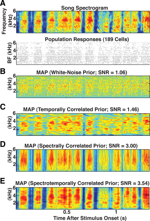
Population decoding of song spectrogram with varying degrees of prior information of song statistics. A, Top, Spectrogram of birdsong played to 189 different neurons leading to the spike responses shown immediately below. Spikes from a given neuron are plotted at the BF at which that neuron's receptive field reaches its maximal value. Neurons with the same BF are plotted on the same row. A–E, MAP estimate given the responses in A using an uncorrelated prior (B), a prior with temporal correlations and no spectral correlations (C), a prior with spectral correlations and no temporal correlations (D), and a prior with spectral and temporal correlations (E). Combining the spike train with spectral information is more important for reconstructing the original spectrogram than combining the spike train with temporal information. However, combining spikes with joint spectrotemporal information leads to the best reconstructions.

Effect of prior information on song estimation

Reconstructions without prior information show discontinuous gaps in power during vocal periods. They also show sparse spectrotemporal correlations at frequencies above 4 kHz. As in the single-neuron case, these features probably reflect the fact that each neuron only filters small spectrotemporal segments of song. In addition, most STRFs have peak frequencies below 4 kHz (this is evident in the plot of spike responses ordered by BF) (Fig. 7B). Intuitively we expect MAP estimates constructed with prior information of song correlations to enhance reconstructions by filling in these “gaps” in power density.

Figure 7 shows how the MAP estimate given the responses from 189 neurons changes as prior information is added. We plot MAP estimates using a prior covariance matrix that contains temporal information but no spectral information (Fig. 7C), spectral information but no temporal information (Fig. 7D), and both spectral and temporal correlations (Fig. 7E) (for details, see Materials and Methods, Birdsong priors) (see Fig. 10 for a plot of preferred frequency tuning across the neural population). Comparing these estimates with the estimate using an uncorrelated prior (Fig. 7B) shows that information about the second-order statistics in zebra finch song enhances reconstructions by interpolating correlations in spectrogram areas not covered by MLd STRFs.

A clear improvement in estimates using the spectrally correlated priors occurs at times where spiking activity is sparse. At these times, the MAP estimate using the uncorrelated prior equals the prior mean. When given knowledge of song correlations, the MAP uses the sparse activity in MLd to correctly infer the deflections from the mean that occur in the original song spectrogram. The correlations also help the MAP infer that, during episodes of high spiking activity, spectral bands above 4 kHz should have similar levels of power as those below 4 kHz. In the supplemental material (available at www.jneurosci.org) we provide the reconstruction in the time domain created by combining the spectrogram in Figure 7E with random phase. For comparison purposes, we also provide the original song constructed with randomized phase.

In Figure 8 we quantify how reconstruction quality improves as a function of the number of neurons used in decoding. We use the SNR (see Materials and Methods) as a quantitative method for evaluating reconstruction accuracy. As described in Materials and Methods, the neurons chosen for reconstruction were randomly chosen from the population.

Figure 8.

Decoding performance given different amounts of prior information and numbers of neurons. A, Spectrogram reconstructions (top) for an example song (Fig. 7A) using a Gaussian prior with spectrotemporal correlations and using varying numbers of neuronal responses (bottom). Above each reconstruction is the SNR used to measure similarity between the reconstructed song and the song presented to the bird. B, Solid lines show the SNR averaged across all decoded songs, whereas dashed lines show 1 SE. The prior used for decoding is denoted by color. Spectral prior information leads to faster growth in the SNR than temporal information. For reference, the magenta line shows the growth in SNR for the commonly used the OLE. The OLE has access to both spectral and temporal correlations. C, Coherence between spectrograms and reconstructions under the four different priors. The horizontal axis reports temporal modulations and the vertical axis reports spectral modulations. All plots display the highest coherence at low spectral and temporal modulations. The primary effect of adding spectrotemporal prior information is to improve reconstructions at lower spectral and temporal modulations.

Figure 8A plots example MAP estimates using the Gaussian prior with spectrotemporal correlations as a function of the number of neurons for a single example song. The associated value of the SNR is given above the MAP estimate. The solid lines in Figure 8B show the SNR averaged across all songs, and dashed lines show the SE about these lines. An SNR value of one corresponds to estimating the spectrogram by a single number, the mean. Improvements in SNR reflect improved estimates in the correlations of song power about the mean. The colors denote which prior was used in computing the MAP estimate. As expected, the SNR from MAP estimates using prior spectrotemporal information (black line) grows the fastest, followed by the SNR from MAP estimates, which use only spectral prior information (green line). The faster growth in SNR using only spectral prior information versus temporal information is probably attributable to the facts that MLd population responses already capture a good deal of temporal information, spectral information helps infer deflections from the mean at times of sparse activity, and most MLd neurons have STRFs with peak frequencies below 4 kHz.

Figure 8C plots the coherence between the reconstructions and original spectrograms. The coherence is a normalized measure of the cross-correlation between the original two-dimensional signal and estimate in the frequency domain. In all of the plots, the vertical axis shows spectral modulations (in units of cycles per kilohertz). These frequencies are often referred to as the ripple density. The horizontal axis shows temporal modulations (in units of hertz). We note that the coherence plot is not the same as the modulation power spectrum shown in Figure 3D. In Figure 8C, the range of the coherence is limited from −10 dB (dark blue), a coherence of 0.1, to 0 dB, i.e., perfect coherence (red). With the exception of the noncorrelated prior, we see a high coherence for temporal modulations between −50 and 50 Hz and ripple densities between 0 and 0.6 cycles/kHz. When we analyzed the coherence within these frequencies, we found that the average coherence is highest for the spectrotemporal prior, second highest for the spectral prior, and smallest for the prior without covariance information. From this plot we conclude that prior knowledge of the stimulus correlations primarily aids in reconstructing lower temporal modulations and ripple densities.

It is interesting to compare the decoding performance just described with the OLE, a simpler and more commonly used decoder (Mesgarani et al., 2009). As discussed in Materials and Methods, the OLE finds the estimate that minimizes the average-squared Euclidean distance between the spectrogram being estimated and a linear combination of the responses. Figure 8 (magenta line) shows the growth in the SNR of the OLE using the same real responses as those used for the nonlinear, Bayesian model. The OLE depends on spectrotemporal correlations in the stimulus so we compare its performance with the prior that contains both spectral and temporal correlations (black line). Comparing these two shows that when the number of neurons is low, the two estimates perform similarly. As more neurons are added to the estimate, the MAP estimator outperforms the OLE. Previous work (Pillow et al., 2011) has shown that this behavior is expected if the encoding model is a good model for spike responses to stimuli and if the prior model does a good job of capturing stimulus correlations. Pillow et al. (2011) showed that when the number of neurons used for estimation is low, the MAP estimate and OLE are equivalent. As the number of neurons grows, the MAP estimate can outperform the OLE because the MAP estimator is not restricted to be a linear function of spike responses.

Hierarchical prior model

We observed visible differences in power density covariance and mean during silent and vocal periods (Fig. 4, covariance matrices, and the differences in color between silent and vocal periods in the plotted spectrograms). These differences are averaged together when constructing the covariance matrix and mean used in the single Gaussian prior. Averaging together the correlation information from these two different periods smoothes the spectral correlation information (compare Figs. 3A, 4B, left, covariance matrices). We reconstructed songs using a hierarchical prior (see Materials and Methods, Hierarchical model prior) to test whether this smoothing hinders the reconstruction performance. This prior includes a state variable that determines the mean and spectral covariance. We first study the case where all possible state trajectories are used for decoding, with trajectory probabilities determined by neural responses and the transition probabilities in our model (see Materials and Methods) (Fig. 4). Each trajectory yields a different reconstructed spectrogram, and the final estimate is determined by averaging across these reconstructions. This is equivalent to estimating the song using the posterior mean. This estimate should be better than an estimate using a single Gaussian if the neural responses provide sufficient information to properly infer state transitions.

In Figure 9A (left) we plot an example song spectrogram with evoked single-neuron, single-trial responses immediately below. We have again plotted the responses at the neuron's best frequency, which in this case is 1.8 kHz. Below this we have plotted the MAP estimate using these responses and a single correlated Gaussian prior (Fig. 9B, top) and the posterior mean using the hierarchical prior (Fig. 9B, bottom). The estimates show surprisingly similar behavior. Under the hierarchical prior, we see power densities slightly closer to those in song, around the neuron's BF, compared to the estimate using a single Gaussian prior. Otherwise, no large differences between the two estimators are seen.

Figure 9.

Single-neuron and population decoding using a hierarchical prior. A, Song spectrogram along with a single cell's response to this song (left) and the response of this cell plus 49 other cells with nearby characteristic frequencies (right). B, MAP estimates using a single, correlated Gaussian prior (top) are compared with estimates using the posterior mean and the hierarchical prior (bottom); in both the single-neuron and population decoding cases, the estimate using a hierarchical prior looks similar to the MAP with a Gaussian prior. C, The expected value for vocalization state given responses; single-cell responses do not yield enough information to accurately infer the spectrogram's vocalization state; however, as the number of neurons used for inference increases, the vocalization state becomes more pronounced.

It is possible that estimates based on the hierarchical model are not much better than those using a single Gaussian because single-neuron responses do not provide enough information to infer the state transitions. Figure 9C shows the average state transition given the neural response. We see that this is indeed the case, and on average, the inferred state transitions do not match those in the song being estimated. Given the above result, we asked whether the hierarchical model would outperform the single Gaussian prior when more neurons are used for decoding. In the right column of Figure 9A, we plot the responses of 49 additional neurons (for a total of 50 neurons) with BFs slightly greater than the single neuron used in the left column. These responses are again plotted below the spectrogram being estimated. Examining the average state changes given responses in Figure 9C, we see a closer resemblance between the inferred state transitions to those present in the estimated song. In the right column of Figure 9B, we plot the posterior mean under the hierarchical prior and the MAP estimate using the same subset of neural responses combined with a single Gaussian (nonhierarchical) prior. The two estimators do not show any prominent differences. Adding more neurons to the estimation should only cause the two estimators to look more similar since the reconstructions will have less dependence on prior information when more data are included. Therefore, we did not compute estimates with >50 neurons using the Hierarchical prior. Finally, we eliminated the portion of reconstruction error caused by problems associated with estimating the state transitions by computing the MAP estimate of the Hierarchical prior given the true underlying state in the song being estimated. We compared this estimate, which has perfect knowledge of the underlying song transitions, to the MAP estimate using a single Gaussian prior. Even in this case, we do not see any large differences between the estimators (data not shown). These results demonstrate that spectrogram estimates do not necessarily improve as more complicated prior information of song is included in the posterior distribution. Although samples from the hierarchical prior contain more statistical information of song and arguably show more resemblance to song than samples from a single, correlated Gaussian prior (compare Figs. 3C, 4C), this advantage does not translate into better spectrogram reconstructions.

Reconstruction dependence On STRF frequency tuning

The information for reconstruction provided by an individual MLd neuron depends on its STRF. Neurons that have STRFs that overlap in their spectrotemporal filtering properties will provide redundant information. Although this redundancy is useful for reducing the noise associated with the spike generation process (Schneider and Woolley, 2010), good spectrogram reconstructions also require enough neurons that provide independent information. We asked whether our results would improve if we used neurons that had either no overlap in their filtering properties or complete overlap. We computed MAP estimates using simulated STRFs, which we will refer to as point STRFs, that have no spectral blur and no history dependence (see Materials and Methods for how these receptive fields were constructed). Figure 10A (top left) plots an STRF calculated from real responses using the method of maximum likelihood (“full” STRF) and a point STRF (top right) with an equivalent peak frequency. In Figure 10A (bottom left), we show the extent of the blurring behavior in our neuronal population. For each neuron, we plot the spectral axis of its STRF at the latency at which that STRF reaches its maximum value. The right panel of Figure 10A shows the same information for the point STRFs (see Materials and Methods for our determination of the number of neurons with a particular peak frequency).

Figure 10B (top) shows an example spectrogram we attempt to reconstruct. For both STRFs, we reconstructed songs using simulated responses. We did not use real responses because we wanted to reduce the differences in reconstruction performance caused by the poorer predictive performance of point STRFs on real data. Using simulated responses allowed us to better control for this effect and focus on differences in reconstruction performance caused by spectral blurring. For comparison purposes, we plot the real responses of 189 neurons, aligned according to their BF, immediately below this spectrogram. The middle panel of Figure 10B shows simulated responses to this example song created using the generalized linear model with point STRFs. The bottom shows simulated responses using full STRFs. Using a correlated Gaussian prior, we reconstructed the spectrogram using the point STRFs and the simulated responses generated from them (middle) and using the full STRFs and their associated simulated responses (bottom).

Stimulus reconstructions using point STRFs show slightly finer spectral detail compared to reconstructions using full STRFs. However, overall we do not find that spectral blurring of the full STRFs leads to much degradation in stimulus reconstructions. The growth in SNR for point STRFs and full STRFs as a function of the number of neurons is shown in Figure 10C. On average, point STRFs have slightly higher signal-to-noise ratios as the number of neurons increases; however, the difference between the two curves is not too great. It is important to point out that these results depend on the fact that reconstructions were performed using a correlated prior trained on natural stimuli. The spectrotemporal width of the covariance is broad compared to that of the full STRFs. When we reconstructed songs using a prior with no correlations, we found that full STRFs decode slightly better than the point STRFs (data not shown). Also, for the reasons stated above, we used simulated responses, which also influences the results. Reconstructions using point STRFs are slightly worse than reconstructions with full STRFs when real data are used. We attribute this difference to the better predictive performance of the full STRFs on real data.

Discussion

We asked whether the responses of zebra finch auditory midbrain neurons to song encode enough information about the stimulus so that an ideal observer of MLd spike trains could recognize and reconstruct the song spectrogram. We found that 189 sequentially recorded MLd responses can be combined using a GLM to discriminate between pairs of songs that are 30 ms in duration with an accuracy equivalent to that found in behavioral experiments. These results are in agreement with prior studies showing that responses from auditory neurons in the forebrain area field L (Wang et al., 2007) and MLd (Schneider and Woolley, 2010) can be used for song discrimination. Importantly, this previous work did not use the GLM to evaluate the discriminability, and thus provides an independent benchmark to compare with our GLM-dependent results.

We tested the hypothesis that the statistics of zebra finch song can be used to perform vocal recognition by decoding MLd responses to conspecific song using a priori knowledge of the joint spectrotemporal correlations present across zebra finch songs. We explicitly used prior information lacking higher-order information of song to test whether MLd responses only require knowledge of correlations to be used for spectrogram reconstruction. When we evaluated the reconstructed spectrograms in the Fourier domain, we found that these responses do a fair job of reproducing temporal and spectral frequencies, i.e., temporal modulations and ripple densities, between −50 and 50 Hz and below 0.6 cycles per kilohertz. When combined with the joint spectrotemporal correlations of zebra finch song, we found an improvement in the coherence in these regions. These results did not change greatly when we used STRFs with nonoverlapping best frequencies, suggesting that the spectral blur or “bandwidth” limitations of the STRF did not strongly affect reconstruction performance using these responses combined with spectrotemporal correlations in zebra finch song.

None of the reconstructions using MLd neurons and the correlations present in song reproduced all the details of a particular spectrogram. These results are qualitatively similar to previous findings showing that the auditory system of zebra finch, as well as other songbirds, can recognize songs even when some of the fine details of the song signal have been degraded by various types of background noise (Bee and Klump, 2004; Appeltants et al., 2005; Narayan et al., 2006; Knudsen and Gentner, 2010). This may be similar to the finding that humans can recognize speech even after the spectral and temporal content has been degraded (Drullman et al., 1994; Shannon et al., 1995).

It is interesting to speculate whether the song features that were reproduced in this study are relevant to the bird for song recognition. For example, we found that reconstructions were most accurate at low ripple densities and temporal modulations. Song recognition based on these features would be consistent with existing evidence that zebra finch are better able to discriminate auditory gratings with lower ripple density/temporal modulations (Osmanski et al., 2009). Because of the complexity of song, it is difficult to quantify behaviorally relevant song features birds use for recognition and communication (Osmanski et al., 2009; Knudsen and Gentner, 2010). The spectrogram reconstructions reported here may serve as a useful probe for future discrimination studies. For example, one could compare discrimination thresholds between songs whose amplitude spectrums have been degraded according to the regions where reconstructions have low coherence and songs whose amplitude spectrums are randomly degraded. If the MAP reconstructions are relevant to the bird, we would expect performance to be worse on songs with randomly degraded amplitude spectrums. This idea is similar to the previously mentioned study by Osmanski et al. (2009) testing discrimination of auditory gratings in birds; however, the ripple density/temporal modulations used for probes would be more complex than simple gratings. Working with ferret auditory cortical neurons, Mesgarani et al. (2009) previously examined the effects of stimulus correlation on spectrogram decoding. Similar to our findings, they found improvements in reconstruction quality when they used prior information of sound correlations. This suggests that the use of natural sound correlations for vocal recognition might be a general strategy used across species. However, there are important distinctions between the Bayesian approach used here for reconstruction and the optimal linear decoder used by Mesgarani et al. (2009). The optimal linear decoder incorporates stimulus correlations via the stimulus–response cross-covariance matrix and the response auto-covariance matrix. The Bayesian decoder incorporates stimulus statistics using a prior distribution that is independent of the likelihood distribution used to characterize neural responses (Eq. 1). Therefore, this decoder allows one to estimate song correlations independent of the amount of neural data available. This is beneficial for obtaining good estimates of song correlations when it is easier to obtain song samples than physiological data. Another important distinction between the linear decoder and the Bayesian method is that the Bayesian decoder does not have to be a linear function of the spike responses. This seems to be the reason for the Bayesian method's slight improvement over the linear decoder. When we decode songs using a linear, Gaussian, Bayesian decoder with the same correlated Gaussian prior as the one in this study, we find worse reconstruction performance than the GLM. This suggests that the nonlinearity is an important factor in the GLM's improved performance.

Another advantage of separating prior information from neural responses is that we could systematically change the before study which statistical properties of song are most important for stimulus reconstruction without refitting the filters applied to the observed spike trains. We found that reconstructions based on MLd responses with a priori information of spectral correlations yielded better estimates of song than did reconstructions using temporal correlations present in song. Although we cannot conclude from this study whether or not the bird actually uses a prior, we speculate that these results suggest what information, in addition to MLd responses, may be used when the bird recognizes song. These results suggest that there is a greater benefit to the bird, in terms of vocal recognition capabilities, if MLd responses are processed by neuronal circuits that have access to the joint spectrotemporal or spectral song correlations rather than temporal correlations. This interpretation would be consistent with previous work showing that zebra finch appear to be more sensitive to frequency cues than temporal cues when categorizing songs belonging to one of two males (Nagel et al., 2010). However, even though much work has been done relating information encoded within a prior distribution to neuronal spiking properties (Zemel et al., 1998; Beck and Pouget, 2007; Litvak and Ullman, 2009), it is unclear how to predict response properties of cells based on the statistical information about a stimulus they may be encoding. To better understand this relationship, future experiments could perform a similar decoding analysis using the responses from other brain areas to look for spiking activity in which it is more beneficial to store temporal correlations rather then spectral correlations. If such activity exists, these responses could be combined with MLd spike trains to perform reconstructions that presumably would only show marginal improvement when combined with prior knowledge of either temporal or spectral correlations.

There has been much recent interest in determining good priors for describing natural sounds and stimuli (Singh and Theunissen, 2003; Karklin and Lewicki, 2005; Cavaco and Lewicki, 2007; McDermott et al., 2009; Berkes et al., 2009). With the two-state model, we briefly explored the effects on reconstruction quality of prior distributions, which contain more information than just the mean and covariance of birdsong; however, none of the priors used in this study explicitly contain information about the subunits such as song notes, syllables, or motifs typically used to characterize song (Catchpole and Slater, 1995; Marler and Slabbekoorn, 2004). Future work could examine whether reconstruction quality changes using more realistic, non-Gaussian prior distributions of birdsong that contain higher-order information. For example, neurons in the songbird forebrain nucleus HVC are known to be sensitive to syllable sequence (Margoliash and Fortune, 1992; Lewicki and Arthur, 1996; Nishikawa et al., 2008), suggesting that there are neural circuits that could provide prior information of sound categories such as syllables and motifs. One could therefore reconstruct songs using this prior information, for example, by using a hidden Markov model with the hidden states trained on sound categories (Kogan and Margoliash, 1998). Although we did not find much of an improvement in reconstruction quality using the two-state prior compared to a Gaussian prior, more realistic priors may yield better reconstructions. If so, one could determine additional statistical information about song stimuli, other than stimulus correlations, also useful for song recognition.

References

- Ahmadian Y, Pillow J, Paninski L. Efficient Markov chain Monte Carlo methods for decoding neural spike trains. Neural Comput. 2011;1:46–96. doi: 10.1162/NECO_a_00059. [DOI] [PMC free article] [PubMed] [Google Scholar]
- Appeltants D, Gentner TQ, Hulse SH, Balthazart J, Ball GF. The effect of auditory distractors on song discrimination in male canaries (Serinus canaria) Behav Processes. 2005;69:331–341. doi: 10.1016/j.beproc.2005.01.010. [DOI] [PubMed] [Google Scholar]
- Beck JM, Pouget A. Exact inferences in a neural implementation of a hidden Markov model. Neural Comput. 2007;19:1344–1361. doi: 10.1162/neco.2007.19.5.1344. [DOI] [PubMed] [Google Scholar]
- Bee MA, Klump GM. Primitive auditory stream segregation: a neurophysiological study in the songbird forebrain. J Neurophysiol. 2004;92:1088–1104. doi: 10.1152/jn.00884.2003. [DOI] [PubMed] [Google Scholar]
- Berkes P, Turner RE, Sahani M. A structured model of video reproduces primary visual cortical organisation. PLoS Comput Biol. 2009;5:e1000495. doi: 10.1371/journal.pcbi.1000495. [DOI] [PMC free article] [PubMed] [Google Scholar]
- Bialek W, Rieke F, de Ruyter van Steveninck R, Warland D. Reading a neural code. Science. 1991;252:1854–1857. doi: 10.1126/science.2063199. [DOI] [PubMed] [Google Scholar]
- Brillinger D. Maximum likelihood analysis of spike trains of interacting nerve cells. Biol Cybern. 1988;59:189–200. doi: 10.1007/BF00318010. [DOI] [PubMed] [Google Scholar]
- Calabrese A, Schumacher J, Schneider D, Woolley SM, Paninski L. A generalized linear model for estimating receptive fields from midbrain responses to natural sounds. Front Neurosci Conference Abstract: Computational and Systems Neuroscience 2010; 2010. [DOI] [Google Scholar]
- Catchpole C, Slater P. Bird song: Biological themes and variations. New York: Cambridge UP; 1995. [Google Scholar]
- Cavaco S, Lewicki MS. Statistical modeling of intrinsic structures in impacts sounds. J Acoust Soc Am. 2007;121:3558–3568. doi: 10.1121/1.2729368. [DOI] [PubMed] [Google Scholar]
- Decharms RC, Blake DT, Merzenich MM. Optimizing sound features for cortical neurons. Science. 1998;280:1439–1443. doi: 10.1126/science.280.5368.1439. [DOI] [PubMed] [Google Scholar]
- Drullman R, Festen JM, Plomp R. Effect of temporal envelope smearing on speech reception. J Acoust Soc Am. 1994;95:1053–1064. doi: 10.1121/1.408467. [DOI] [PubMed] [Google Scholar]
- Eggermont J. Between sound and perception: reviewing the search for a neural code. Hear Res. 2001;157:1–42. doi: 10.1016/s0378-5955(01)00259-3. [DOI] [PubMed] [Google Scholar]
- Eggermont JJ, Aertsen AM, Johannesma PI. Quantitative characterization procedure for auditory neurons based on the spectro-temporal receptive field. Hear Res. 1983;10:167–190. doi: 10.1016/0378-5955(83)90052-7. [DOI] [PubMed] [Google Scholar]
- Gentner TQ, Margoliash D. The neuroethology of vocal communication: perception and cognition. New York: Springer; 2002. Acoustic communication; pp. 324–386. Chap 7. [Google Scholar]
- Godard R. Long-term memory for individual neighbors in a migratory songbird. Nature. 1991;350:228–229. [Google Scholar]
- Hauber M, Campbell D, Woolley SM. Functional role and female perception of male song in zebra finches. EMU. 2010;110:209–218. [Google Scholar]
- Hesselmans GH, Johannesma PI. Spectro-temporal interpretation of activity patterns of auditory neurons. Math Biosci. 1989;93:31–51. doi: 10.1016/0025-5564(89)90012-6. [DOI] [PubMed] [Google Scholar]
- Karklin Y, Lewicki MS. A hierarchical Bayesian model for learning nonlinear statistical regularities in nonstationary natural signals. Neural Comput. 2005;17:397–423. doi: 10.1162/0899766053011474. [DOI] [PubMed] [Google Scholar]
- Knudsen DP, Gentner TQ. Mechanisms of song perception in oscine birds. Brain Lang. 2010;1:59–68. doi: 10.1016/j.bandl.2009.09.008. [DOI] [PMC free article] [PubMed] [Google Scholar]
- Kogan JA, Margoliash D. Automated recognition of bird song elements from continuous recordings using dynamic time warping and hidden Markov models: A comparative study. J Acoust Soc Am. 1998;103:2185–2196. doi: 10.1121/1.421364. [DOI] [PubMed] [Google Scholar]
- Koyama S, Eden UT, Brown EN, Kass RE. Bayesian decoding of neural spike trains. Ann Inst Stat Math. 2010;62:37–59. [Google Scholar]
- Lee SI, Lee H, Abbeel P, Ng AY. Efficient L1 regularized logistic regression. Proceedings of the Twenty-First National Conference on Artificial Intelligence; Boston: Association for the Advancement of Artificial Intelligence; 2006. pp. 401–408. [Google Scholar]
- Lehmann EL, Romano JP. Testing statistical hypotheses. New York: Springer; 2005. [Google Scholar]
- Lewicki MS, Arthur BJ. Hierarchical organization of auditory temporal context sensitivity. J Neurosci. 1996;16:6987–6998. doi: 10.1523/JNEUROSCI.16-21-06987.1996. [DOI] [PMC free article] [PubMed] [Google Scholar]
- Litvak S, Ullman S. Cortical circuitry implementing graphical models. Neural Comput. 2009;21:3010–3056. doi: 10.1162/neco.2009.05-08-783. [DOI] [PubMed] [Google Scholar]
- Lohr B, Dooling R. Detection of changes in timbre and harmonicity in complex sounds by zebra finches (Taeniopygia guttata) and budgerigars (Melopsittacus undulatus) J Comp Psychol. 1998;112:36–47. doi: 10.1037/0735-7036.112.1.36. [DOI] [PubMed] [Google Scholar]
- Margoliash D, Fortune ES. Temporal and harmonic combination-sensitive neurons in the zebra finch's HVc. J Neurosci. 1992;12:4309–4326. doi: 10.1523/JNEUROSCI.12-11-04309.1992. [DOI] [PMC free article] [PubMed] [Google Scholar]
- Marler PR, Slabbekoorn H. Nature's music: the science of birdsong. London: Elsevier Academic; 2004. [Google Scholar]
- McCullagh P, Nelder JA. Generalized linear models. Ed 2. London: Chapman and Hall/CRC; 1989. [Google Scholar]
- McDermott JH, Oxenham AJ, Simoncelli EP. IEEE Workshop on Applications of Signal Processing to Audio and Acoustics. IEEE: New Paltz, NY; 2009. Sound texture synthesis via filter statistics. October. [Google Scholar]
- Mesgarani N, David SV, Fritz JB, Shamma SA. Influence of context and behavior on stimulus reconstruction from neural activity in primary auditory cortex. J Neurophysiol. 2009;102:3329–3339. doi: 10.1152/jn.91128.2008. [DOI] [PMC free article] [PubMed] [Google Scholar]
- Nagel KI, McLendon HM, Doupe AJ. Differential influence of frequency, timing, and intensity cues in a complex acoustic categorization task. J Neurophysiol. 2010;104:1426–1437. doi: 10.1152/jn.00028.2010. [DOI] [PMC free article] [PubMed] [Google Scholar]
- Narayan R, Grana G, Sen K. Distinct time scales in cortical discrimination of natural sounds in songbirds. J Neurophysiol. 2006;96:252–258. doi: 10.1152/jn.01257.2005. [DOI] [PubMed] [Google Scholar]
- Nishikawa J, Okada M, Okanoya K. Population coding of song element sequence in the Bengalese finch HVc. Eur J Neurosci. 2008;27:3273–3283. doi: 10.1111/j.1460-9568.2008.06291.x. [DOI] [PubMed] [Google Scholar]
- O'Loghlen AL, Beecher MD. Sexual preferences for mate song types in female song sparrows. Anim Behav. 1997;53:835–841. [Google Scholar]
- Osmanski MS, Marvit P, Depireux DA, Dooling RJ. Discrimination of auditory gratings in birds. Hear Res. 2009;256:11–20. doi: 10.1016/j.heares.2009.04.020. [DOI] [PMC free article] [PubMed] [Google Scholar]
- Paninski L. Maximum likelihood estimation of cascade point-process neural encoding models. Network. 2004;15:243–262. [PubMed] [Google Scholar]
- Paninski L, Ahmadian Y, Ferreira D, Koyama S, Rahnama K, Vidne M, Vogelstein J, Wu W. A new look at state-space models for neural data. J Comp Neurosci. 2009;29:107–126. doi: 10.1007/s10827-009-0179-x. [DOI] [PMC free article] [PubMed] [Google Scholar]
- Peek FW. An experimental study of the territorial function of vocal and visual display in the male red-winged blackbird (Agelaius phoeniceus) Anim Behav. 1972;20:112–118. doi: 10.1016/s0003-3472(72)80181-7. [DOI] [PubMed] [Google Scholar]
- Percival DB, Walden AT. Spectral analysis for physical applications: Multitaper and conventional univariate techniques. Cambridge, UK: Cambridge UP; 1993. [Google Scholar]
- Pillow J, Ahmadian Y, Paninski L. Model-based decoding, information estimation, and change-point detection in multi-neuron spike trains. Neural Comput. 2011;1:1–45. doi: 10.1162/NECO_a_00058. [DOI] [PubMed] [Google Scholar]
- Rieke F, Bodnar DA, Bialek W. Naturalistic stimuli increase the rate and efficiency of information transmission by primary auditory afferents. Proc R Soc Lond B Biol Sci. 1995;262:259–265. doi: 10.1098/rspb.1995.0204. [DOI] [PubMed] [Google Scholar]
- Rieke F, Warland D, de Ruyter Bialek W. Spikes: exploring the neural code. Cambridge, MA: MIT; 1997. [Google Scholar]
- Robert C, Casella G. Monte Carlo statistical methods. New York: Springer; 2005. [Google Scholar]
- Schneider D, Woolley SM. Discrimination of communication vocalizations by single neurons and groups of neurons in the auditory midbrain. J Neurophysiol. 2010;6:3248–3265. doi: 10.1152/jn.01131.2009. [DOI] [PMC free article] [PubMed] [Google Scholar]
- Sen K, Theunissen FE, Doupe AJ. Feature analysis of natural sounds in the songbird auditory forebrain. J Neurophysiol. 2001;86:1445–1458. doi: 10.1152/jn.2001.86.3.1445. [DOI] [PubMed] [Google Scholar]
- Shannon RV, Zeng FG, Kamath V, Wygonski J, Ekelid M. Speech recognition with primarily temporal cues. Science. 1995;270:303–304. doi: 10.1126/science.270.5234.303. [DOI] [PubMed] [Google Scholar]
- Shinn-Cunningham BG, Best V, Dent ML, Gallun FJ, Mcclaine EM, Narayan R, Sen K. Behavioral and neural identification of birdsong under several masking conditions. Berlin: Springer; 2007. [Google Scholar]
- Singh N, Theunissen F. Modulation spectra of natural sounds and ethological theories of auditory processing. J Acoustical Soc Am. 2003;114:3394–3411. doi: 10.1121/1.1624067. [DOI] [PubMed] [Google Scholar]
- Theunissen FE, Shaevitz SS. Auditory processing of vocal sounds in birds. Curr Opin Neurobiol. 2006;16:400–407. doi: 10.1016/j.conb.2006.07.003. [DOI] [PubMed] [Google Scholar]
- Theunissen FE, Sen K, Doupe AJ. Spectral-temporal receptive fields of nonlinear auditory neurons obtained using natural sounds. J Neurosci. 2000;20:2315–2331. doi: 10.1523/JNEUROSCI.20-06-02315.2000. [DOI] [PMC free article] [PubMed] [Google Scholar]
- Theunissen F, David S, Singh N, Hsu A, Vinje W, Gallant J. Estimating spatiotemporal receptive fields of auditory and visual neurons from their responses to natural stimuli. Network. 2001;12:289–316. [PubMed] [Google Scholar]
- Truccolo W, Eden U, Fellows M, Donoghue J, Brown E. A point process framework for relating neural spiking activity to spiking history, neural ensemble and extrinsic covariate effects. J Neurophysiol. 2005;93:1074–1089. doi: 10.1152/jn.00697.2004. [DOI] [PubMed] [Google Scholar]
- Wang L, Narayan R, Grana G, Shamir M, Sen K. Cortical discrimination of complex natural stimuli: Can single neurons match behavior? J Neurosci. 2007;27:582–589. doi: 10.1523/JNEUROSCI.3699-06.2007. [DOI] [PMC free article] [PubMed] [Google Scholar]
- Warland D, Reinagel P, Meister M. Decoding visual information from a population of retinal ganglion cells. J Neurophysiol. 1997;78:2336–2350. doi: 10.1152/jn.1997.78.5.2336. [DOI] [PubMed] [Google Scholar]
- Woolley SM, Gill PR, Fremouw T, Theunissen FE. Functional groups in the avian auditory system. J Neurosci. 2009;29:2780–2793. doi: 10.1523/JNEUROSCI.2042-08.2009. [DOI] [PMC free article] [PubMed] [Google Scholar]
- Woolley S, Gill P, Theunissen F. Stimulus-dependent auditory tuning results in synchronous population coding of vocalizations in the songbird midbrain. J Neurosci. 2006;26:2499–2512. doi: 10.1523/JNEUROSCI.3731-05.2006. [DOI] [PMC free article] [PubMed] [Google Scholar]
- Zemel R, Dayan P, Pouget A. Probabilistic interpretation of population codes. Neural Comput. 1998;10:403–430. doi: 10.1162/089976698300017818. [DOI] [PubMed] [Google Scholar]