Development and Validation of Transferable Amide I Vibrational Frequency Maps for Peptides

Abstract

Infrared (IR) spectroscopy of the amide I band has been widely utilized for the analysis of peptides and proteins. Theoretical modeling of IR spectra of proteins requires an accurate and efficient description of the amide I frequencies. In this paper, amide I frequency maps for protein backbone and side chain groups are developed from experimental spectra and vibrational lifetimes of N-methylacetamide and acetamide in different solvents. The frequency maps, along with established nearest-neighbor frequency shift and coupling schemes, are then applied to a variety of peptides in aqueous solution and reproduce experimental spectra well. The frequency maps are designed to be transferable to different environments; therefore, they can be used for heterogeneous systems, such as membrane proteins.

I. INTRODUCTION

Proteins play essential roles in biological processes, functioning as structural supporters, catalysts, signal transmitters, and so on.^1–3 Their biological functions are determined by their three-dimensional structures, which undergo constant motions over a wide range of time and length scales.^4,5 The structure and dynamics of proteins can be probed by a variety of experimental techniques. X-ray crystallography is used to determine the complete three-dimensional structure of proteins at high resolution,^6,7 as long as the proteins can be crystallized. Nuclear magnetic resonance spectroscopy measures protein structure in solution at the atomic level and has greatly enriched our understanding of how proteins fold and interact with other molecules.^5,8 Other techniques, such as Raman, circular dichroism, electron paramagnetic resonance, and ultraviolet absorption and fluorescence spectroscopy are also commonly used for the analysis of proteins.^9–13

Infrared (IR) spectroscopy is another sensitive and versatile technique for studying the structure and dynamics of proteins under a variety of sample conditions, such as in aqueous solution or lipid membranes.^14,15 In IR experiments, the amide I vibrational mode, primarily associated with the peptide bond carbonyl stretch,¹⁴ is often utilized for structural analysis. Each local amide I mode is called a chromophore, and the many chromophores in a peptide or protein couple together to form the amide I band. The frequencies at which the amide I band occur, along with the band widths and intensities, depend on different patterns of intra- and intermolecular couplings. Thus, different protein secondary structures have characteristic spectral features in the amide I region (1600–1700 cm⁻¹).^16–18 For example, α-helices absorb near 1650 cm⁻¹, whereas β-sheets have two bands at ~1620 and 1675 cm⁻¹. Recent development of time-resolved two-dimensional infrared (2DIR) spectroscopy has enabled the measurement of molecular dynamics over picosecond time scales and also provides a more detailed picture of the couplings among chromophores.^19–25 Moreover, residue-specific information can be revealed by the isotope-labeling technique. For example, ¹³C and ¹³C=¹⁸O isotope labels lower the amide I frequency by ~40 and 70 cm⁻¹, respectively.^26–40 Carbonyls with isotope labels are essentially shifted out of the main amide I band and can be resolved individually.

The detailed interpretation of experimental spectra is facilitated by theoretical calculations. Modern calculations of vibrational spectra for the amide I region of proteins in complex environments treat the amide stretches quantum mechanically and all other nuclear degrees of freedom, classically.^41–77 For IR absorption spectra, which involve only one quantum of amide vibrational excitation, a central quantity is the one-exciton Hamiltonian and its dependence on the classical degrees of freedom (which evolve in time according to a classical molecular dynamics (MD) simulation). The diagonal terms of this Hamiltonian correspond to the transition frequencies of the local amide chromophores, whereas the off-diagonal terms involve the couplings between pairs of chromophores.

For each configuration of the classical coordinates (each time step in the MD simulation), the exciton Hamiltonian can, in principle, be determined from ab initio electronic structure calculations,^78–80 but in practice, it is impossible to perform accurate enough calculations for peptides in solution or membranes for the very large number of configurations required for computing line shapes. This has led to the development of ab initio-based coupling and frequency “maps”. These are most conveniently discussed by first considering model peptides in the gas phase. Electronic structure calculations are performed for a grid of the relevant dihedral angles. For each set of dihedral angles, the exciton Hamiltonian is determined from the normal modes through the Hessian matrix reconstruction approach.^{42,45,47,50,52,67,72,81,82} This then leads to nearest-neighbor frequency shift (NNFS) maps,⁶⁷ which show explicitly how the local chromophore’s frequency depends on the neighboring dihedral angles. It also leads to coupling maps for both nearest neighbors (the nearest-neighbor coupling (NNC) maps)^42,67 and chromophores that are more distant (through the transition dipole coupling (TDC) approach).^{14,41,42,45,62,64,67,73,74,83–86}

The second step is to include the effects of environmental perturbations, from water, ions, lipids, etc. on the local chromophore frequencies. These are also conveniently expressed as frequency maps.^{46,49,55–58,60,64,66,68,69} Numerous maps have been developed for the amide I vibrational frequencies of protein backbone chromophores in condensed phase, mostly by considering N-methylacetamide (NMA), a molecule with a single amide I chromophore, in water. Experimentally, heavy water (D₂O) is commonly used instead of water to avoid the interference of the water bend mode (~1640 cm⁻¹) with the amide I band. The major isotopic form of NMA in D₂O is N-deuterated NMA (NMAD), as shown in Figure 1a. By performing electronic structure calculations on clusters of NMAD surrounded by D₂O, frequency maps have been developed that relate the amide I frequency to the electric potential^{46,49,55,56,64,66} or electric field^{57,58,60,68,69} on different atom sites from the surrounding solvent molecules.

Figure 1.

Molecular structures of (a) NMAD, (b) ACED, (c) AAO, and (d) AGO.

One example of a field map was developed by Schmidt et al.⁵⁷ In their development, classical MD simulations of NMAD in D₂O were performed, and representative NMAD/D₂O clusters were extracted. For each cluster, ab initio calculations were carried out to obtain the amide I frequency of NMAD. The frequency was assumed to be linear in the electric fields on the NMAD atoms, and the coefficients were determined by multiple linear regression to the ab initio frequencies. The resulting frequency map includes electric fields on the C, O, N, and D atoms, with the largest coefficients on the C and N atoms in the C=O bond direction. Following the same procedure, Lin et al.⁵⁸ simplified the map by fixing the zero-field intercept at the gas-phase absorption frequency of NMAD and incorporating electrostatic contributions only on the C and N atoms in the C=O bond direction. This map is termed as S2 in the following. Both maps reproduced the experimental IR absorption spectrum of NMAD in D₂O fairly well.

Nonetheless, discrepancies between theoretical and experimental spectra reveal problems associated with ab initio-based maps. For example, the level of theory and size of basis set will influence the accuracy of the maps, and the cluster sizes chosen are rather limited and do not account for the entire solvent effect. To circumvent these problems, Lin et al.⁵⁸ switched to an empirical approach. Assuming the same form of S2, they reoptimized the coefficients using the experimental spectrum of NMAD in D₂O. This empirical map was applied to a transmembrane peptide, CD3ζ,⁵⁸ the M2 proton channel of the influenza A virus,³⁹ and an antimicrobial peptide ovispirin⁴⁰ and reproduced the experimental 2DIR diagonal line widths quite well. This approach is appealing in that although its simple functional form is based on ab initio calculations, the parameters are chosen to ensure that it is the best frequency map compared with experiment for a given force field. A drawback of this map is that it is not necessarily transferable to different environments, mainly because it was parametrized in a single solvent (D₂O).

To ameliorate this situation, we present here a new empirical frequency map for protein backbone modes. Again assuming the S2 form, but relaxing the constraint that the zero-field intercept reproduce the gas-phase frequency, the coefficients are optimized from experimental spectra and vibrational lifetimes of NMAD in the three solvents D₂O, DMSO, and CHCl₃, each representing a different electrostatic environment. Using the dielectric constant ε as a rough measure of the solvent’s polarity, these three solvents range from a highly polar environment (water, ε = 78.5); to a polar but aprotic environment (DMSO, ε = 47.2); and finally, to a nearly nonpolar environment (chloroform, ε = 4.8).

Asparagine (Asn) and glutamine (Gln) have amide groups in their side chains, and their absorption spectra contribute to the amide I region. Therefore, for peptides containing these residues, it is also important to include them in the exciton Hamiltonian and provide maps for them. These side chain groups have two hydrogen-bonding sites at the amide hydrogen atoms, so distributions of surrounding solvent molecules are quite different from those around backbone amide I chromophores. Therefore, the backbone map will not necessarily describe these side chains well. We have chosen N-deuterated acetamide (ACED, as shown in Figure 1b) as a model system and use spectra from it to develop a side chain map. Note that as these new backbone and side chain maps are designed to be transferable to different environments; they are potentially applicable to heterogeneous systems, such as membrane proteins.

Armed with these new transferable backbone and side chain frequency maps and existing protocols for NNFS and NNC maps,⁶⁷ as well as TDC for longer range interactions,⁴² we next validate these maps by comparing to experimental spectra for a number of quite different model peptides. Specifically, we first consider simple molecules with one backbone and one side chain chromophore. Next, we consider the α-helical peptide AKA, with and without isotope labels;^32,87 the Trpzip2 peptide, with and without isotope labels;^88,89 and the rat and human versions of islet amyloid polypeptide (IAPP).^90,91 In all cases, agreement between theory and experiment, without any ad hoc frequency shifts or further adjustments, is very good. The paper is organized as follows: In Section II, we describe the mixed quantum/classical treatment of the line shape theory and give the formula used for line shape calculations in this work. We also describe experimental details for spectra and lifetime measurements. Section III presents the development of the frequency maps. Validations of the maps are discussed in Sections IV and V. Finally, conclusions are drawn in Section VI.

II. MATERIALS AND METHODS

A. Line Shape Theory

The absorption line shape can be written as the Fourier transform of the quantum dipole time-correlation function.⁹² If the electric field of the excitation light is polarized in the ε̂ direction, the linear absorption line shape is

$$I(\omega )\sim Re{\int }_0^{\infty }\text{d}t{e}^{-i\omega t}\langle \widehat{\epsilon }·\overrightarrow{\mu }(0)\overrightarrow{\mu }(t)·\widehat{\epsilon }\rangle$$ (1)

where μ⃗ is the dipole operator of the system. The brackets indicate a quantum equilibrium statistical mechanical average, which is impossible to evaluate for proteins in a condensed phase.

As discussed before, one practical approximation is to treat the amide I subspace quantum mechanically, ignore other high-frequency modes, and treat the low-frequency degrees of freedom (translations, rotations, and torsions) classically. Within such a mixed quantum/classical approach, the IR line shape for a multichromophore system is^93,94

$$I(\omega )\sim Re{\int }_0^{\infty }\text{d}t{\text{e}}^{-i\omega t}\sum _{ij}\langle m_i(0)F_{ij}(t)m_j(t)\rangle {\text{e}}^{-t/2T_1}$$ (2)

In the above equation, i and j index the amide I vibrational chromophore; m_i(t) = m⃗_i(t) · ε̂, where m⃗_i(t) is the transition dipole of the ith chromophore at time t. The Hamiltonian (divided by ħ) in the amide I subspace is

$${\kappa }_{ij}(t)={\omega }_i(t){\delta }_{ij}+{\omega }_{ij}(t)(1-{\delta }_{ij})$$ (3)

where ω_i(t) are the local-mode transition frequencies and ω_ij(t) are the vibrational couplings. The matrix F(t) is the time-evolution operator for the one-exciton Hamiltonian,

$$\stackrel{.}{F}(t)=iF(t)\kappa (t)$$ (4)

and it satisfies the initial condition F_ij(0) = δ_ij. The angular brackets now indicate a classical equilibrium statistical mechanical average. T₁ is the lifetime of the first excited state of an isolated amide I vibration, and the term e^−t/2T₁ is added phenomenologically to incorporate lifetime broadening. Equation 2 will be used to calculate theoretical line shapes for the different peptides.

In the map development, both model systems NMAD and ACED contain a single chromophore. For such single-chromophore systems, eq 2 becomes⁹³

$$I(\omega )\sim Re{\int }_0^{\infty }\text{d}t{\text{e}}^{-i\omega t}\langle mk(0)m(t){\text{e}}^{i{\int }_0^t\omega (t^{\prime }){\text{d}t}^{\prime }}\rangle {\text{e}}^{-t/2T_1}$$ (5)

If the frequency fluctuation from its average, δω(t) = ω(t) − 〈ω〉, follows Gaussian statistics, the absorption line shape can be related to the frequency fluctuation time-correlation function, C(t) = 〈δω(t) δω(0)〉. If one makes the cumulant and Condon approximations and neglects orientational dynamics, the IR line shape can be simplified as^58,95,96

$$I(\omega )\sim Re{\int }_0^{\infty }\text{d}t{\text{e}}^{-i(\omega -\langle \omega \rangle )t}{\text{e}}^{-g(t)}{\text{e}}^{-t/2T_1}$$ (6)

where

$$g(t)\equiv {\int }_0^t{\text{d}t}^{\prime }(t-t^{\prime })C(t^{\prime })$$ (7)

This approximation is particularly useful for our map development, since g(t) can be calculated easily for different map parameters.

Actually, the experiments show that vibrational population relaxation is not single-exponential, but rather, is biexponential. Therefore, we modify the above appropriately,⁹⁷

$$I(\omega )\sim Re{\int }_0^{\infty }\text{d}t{\text{e}}^{-i(\omega -\langle \omega \rangle )t}{\text{e}}^{-g(t)}\left\{f{\text{e}}^{-t/2T_s}+(1-f){\text{e}}^{-t/2T_l}\right\}$$ (8)

where T_s and T_l are the “short” and “long” lifetimes, respectively, and f is the amplitude of the fast contribution.

B. Experimental IR Spectra and Pump–Probe Measurements

NMA and acetamide were purchased from Aldrich. NMAD and ACED were obtained by dissolving the samples in D₂O, removing D₂O by speed vacuum concentration, and repeating this procedure three times. FTIR spectra in the three different solvents were taken in an IR cell, with CaF₂ windows separated by a 100 μm Teflon spacer. The concentrations of NMAD and ACED for FTIR measurements were ~20 mM.

Lifetimes were determined through mid-IR pump–probe transient absorption measurements. The femtosecond laser system and optical parametric amplifier used to generate 60 fs mid-IR pulses has been described previously.⁹⁸ The mid-IR pulses were split into pump and probe pulses with 1 μJ and 0.2 μJ pulses energies, respectively, at the sample. The pump pulse polarization was set at 54.7° (magic angle) relative to the probe pulse to eliminate rotational dynamics from the measured kinetics. The pump pulses were chopped at 500 Hz using a mid-IR pulse shaper.⁹⁹ Measurements were made at a series of sample concentrations and checked for consistency to eliminate effects due to self-association. The pump–probe spectrum was recorded as an average over 20–30 scans of the time delay between pump and probe pulses. Transient kinetics at the bleach maxima were fit to a biexponential function convoluted with a Gaussian instrument response function using a nonlinear least-squares fitting routine with the Levenberg–Marquardt algorithm. The standard deviation at each time delay was used as a weighting factor in the fitting routine, and the resulting uncertainties in the fit parameters are reported as twice the standard deviation.

In Table 1, we report the experimental lifetimes and amplitudes, for NMAD in DMSO and chloroform and ACED in DMSO and D₂O (but not in chloroform; see below). The results for NMAD in D₂O are taken from DeCamp et al.⁹⁷ DeCamp et al. also studied NMA in DMSO-d₆ and CDCl₃, but concluded that H/D exchange had not fully occurred, so they were actually studying NMA (rather NMAD). In Table 2, we report the experimental peak frequencies, ω, and full-width-half-maxima, Γ.

Table 1.

Biexponential Fit Parameters from the Pump-Probe Measurements of NMAD and ACED in Different Solvents

solute	solvent	f	Ts (ps)	Tl (ps)
NMAD	D2O 97	0.55	0.20 ± 0.02	0.86 ± 0.09
NMAD	DMSO	0.778	0.66 ± 0.09	3.1 ± 0.7
NMAD	CHCl3	0.769	1.06 ± 0.10	5.2 ± 0.7
ACED	D2O	0.753	0.13 ± 0.05	1.01 ± 0.11
ACED	DMSO	0.651	0.39 ± 0.05	2.27 ± 0.12

Table 2.

Summary of Simulated and Experimental IR Line Shape Parameters for NMAD and ACED in Different Solvents^a

	ωD2O	ΓD2O	ωDMSO	ΓDMSO	ωCHCl3	ΓCHCl3
sim (NMAD)	1621	34	1656	22	1668	16
exptl (NMAD)	162397	2897	1659	23	1665	26
sim (ACED)	1634	40	1666	22	1697
exptl (ACED)	1633	37	1664	22	1700

^aAll quantities are in units of cm⁻¹.

III. DEVELOPMENT OF THE EMPIRICAL AMIDE I FREQUENCY MAPS

The GROMOS96 53a6 force field^100–102 has been extensively used in biological simulations.^{90,91,103,104} In this work, transferable frequency maps for protein backbone and side chain amide chromophores are developed using this force field. We assume the same form of the ab initio-based S2 map,^57,58

$${\omega }_i={\omega }_0+{aE}_{\text{C}i}+{bE}_{\text{N}i}$$ (9)

ω_i is the instantaneous frequency for the ith chromophore, E_Ci is the electric field on the C atom in the ith chromophore along the C=O bond direction, and E_Ni is that on the N atom. Parameters ω₀, a, and b are obtained such that they optimally reproduce the experimental IR absorption spectra of NMAD or ACED in different solvents. Note that the intercept ω₀ is allowed to vary instead of being fixed to the gas-phase absorption frequency. ω₀ is the amide I frequency with no external field. Because we are mainly interested in condensed-phase systems, such a zero-field environment usually represents a nonpolar environment in which nonelectrostatic forces, such as dispersion, dominate. In the GROMOS96 53a6 force field, examples include alkanes, CCl₄, and the hydrophobic tails of lipids. Thus, we allow ω₀ to vary to take those nonelectrostatic effects into account, and thus, ideally the map will reproduce the experimental frequency of NMAD or ACED in those environments.

A. Backbone Frequency Map

NMAD is used as a model compound for the protein backbone amide linkage. Its structure is shown in Figure 1a. NVT MD simulations of NMAD in the solvents D₂O, DMSO, or CHCl₃ were performed at 298 K using the GROMACS simulation package,^105–109 with the GRO-MOS96 53a6 force field.^100–102 In each case, the experimental solvent density determined the simulation volume. The LINCS algorithm¹¹⁰ was used to constrain all bonds in the NMAD/D₂O and NMAD/CHCl₃ systems, and the SHAKE algorithm¹¹¹ was used for NMAD/DMSO. Particle-mesh Ewald (PME)^112,113 was used to calculate the long-range Coulombic interactions. After equilibration, 2 ns production runs with a 2 fs time step were performed. Electric fields on the C and N atoms from solvent molecules within 20 Å were calculated. The line shapes were obtained from eq 8, using the experimental lifetime parameters for NMAD in the three solvents.

The parameters ω₀, a, and b are determined by the Fletcher–Reeves–Polak–Ribiere method,¹¹⁴ which globally minimizes

$${\xi }^2=\sum _{\alpha =1}^3\left\{\frac{{(\mathrm{\Delta }{\omega }_{\alpha }-\mathrm{\Delta }{\omega }_{\alpha ,exp})}^2}{\mathrm{\Delta }{\omega }_{\alpha ,exp}^2}+\frac{{({\mathrm{\Gamma }}_{\alpha }-{\mathrm{\Gamma }}_{\alpha ,exp})}^2}{{\mathrm{\Gamma }}_{\alpha ,exp}^2}\right\}$$ (10)

“1”, “2”, and “3” denote D₂O, DMSO, and CHCl₃, respectively. Δω_α = ω_α − ω_g, which is the frequency shift from the gas phase value of NMAD (1717 cm⁻¹).¹¹⁵ As noted earlier, the experimental line shape parameters are shown in Table 2. The amide I peak frequency of NMAD varies by ~40 cm⁻¹ between D₂O and CHCl₃, showing that the solvents chosen represent different electrostatic environments and the amide I mode is sensitive enough to distinguish among them.

The optimized backbone map is

$${\omega }_i=1684+7729E_{\text{C}i}-3576E_{\text{N}i}$$ (11)

In the above equation, ω_i is in cm⁻¹ and E_Ci and E_Ni are in atomic units. The calculated IR line shapes for NMAD using this map (shown in Table 2 and Figure 2a) are in good agreement with experiment. Note, in particular, that the deviation between experiment and theory for the peak frequency is, at most, 3 cm⁻¹.

Figure 2.

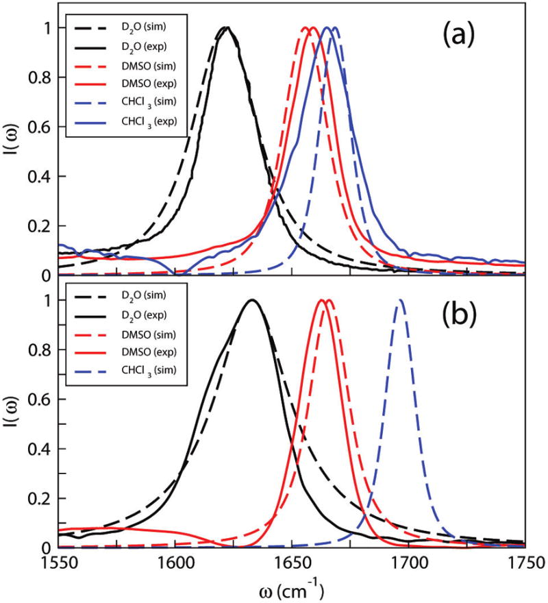
Simulated and experimental absorption spectra of (a) NMAD and (b) ACED in different solvents. The experimental spectrum of NMAD in D₂O is from DeCamp et al.⁹⁷ The experimental spectrum of ACED in CHCl₃ has two peaks and is not shown in the figure.

The map has coefficients a and b with opposite signs, which we can understand as follows. It is generally accepted that the NMAD molecule has three hydrogen-bonding sites and that hydrogen bonds lead to red shifts in local frequencies.^{46,49,50,55,57} The two water molecules hydrogen-bonded to the amide oxygen produce negative (opposite to the CO direction) electric fields on the C atom, and thus, the term +7729E_Ci corresponds to a red shift due to these hydrogen bonds. Similarly, the water molecule hydrogen-bonded to the amide deuterium causes a positive electric field on the N atom, and from eq 11, it also leads to a red shift.

In a nonpolar environment, the map predicts a frequency of 1684 cm⁻¹. Experimentally, spectra for NMA in the nonpolar solvents n-hexane and CCl₄ peak at 1697 and 1688 cm⁻¹, respectively.^116–118 Because NMAD is expected to have a similar (but slightly red-shifted) absorption compared with NMA,¹¹⁷ the map gives a reasonable result for nonpolar solvents.

B. Side Chain Map

We develop a side chain map from ACED following similar procedures. The minimization function is chosen to be

$${\xi }^2={({\omega }_1-{\omega }_{1,exp})}^2+{({\mathrm{\Gamma }}_1-{\mathrm{\Gamma }}_{1,exp})}^2+{({\omega }_2-{\omega }_{2,exp})}^2+{({\mathrm{\Gamma }}_2-{\mathrm{\Gamma }}_{2,exp})}^2+{({\omega }_3-{\omega }_{3,exp})}^2$$ (12)

Absolute peak positions are used in this case because no experimental gas-phase absorption spectrum of ACED is available. The line width in CHCl₃ is not included in the above equation because of self-association of ACED in this solvent. ACED shows two peaks in chloroform, similar to its undeuterated counterpart.^119,120 The strongly overlapped peaks are attributed to monomeric and associated ACED species, with the former absorbing at ~1700 cm⁻¹, and the line width is not well resolved.

The optimized side chain map is

$${\omega }_i^{\text{s}}=1714+2154E_{\text{C}i}+3071E_{\text{N}i}$$ (13)

and the line shape results are shown in Table 2 and Figure 2b. As seen, the experimental and theoretical spectra are in excellent agreement. Note, however, that the experimental spectrum for ACED in D₂O shows a shoulder on the red side not captured by theory. Calculations without making the cumulant approximation (not shown) also do not produce this shoulder. Also note that the calculated peak frequency in chloroform is 1697 cm⁻¹, in good agreement with the monomer absorption discussed above. Unlike the backbone map, for this side chain map, a and b have the same sign. Solvent molecules distribute differently around ACED compared with NMAD. In ACED, the –ND₂ group can form two hydrogen bonds, and the resulting electric field on the N atom depends on the hydrogen-bond angles; thus, E_Ni is not necessarily positive. The zero-field intercept is checked by comparing with spectra for undeuterated acetamide (ACE) in a nonpolar solvent. ACE absorbs at 1714 cm⁻¹ in CCl₄,^121,122 and it is expected that ACED will have similar behavior, which corresponds well to the zero-field intercept of 1714 cm⁻¹.

IV. VALIDATION OF BACKBONE AND SIDE CHAIN MAPS: ONE- AND TWO-CHROMOPHORE SYSTEMS

A. Temperature Dependence of the Amide I Peak Frequency of NMAD in D₂O

Experimentally, it has been shown by Amunson and Kubelka¹²³ that the NMAD amide I peak frequency in D₂O is a very weak function of temperature, increasing by only 6 cm⁻¹ as the temperature varies between 0 and 85 °C. As a check of the map and probably even more of the GROMOS 53a6 force field (which uses the SPC potential¹²⁴ for water), it is interesting to see what our map predicts for the frequency shift with temperature. To this end, 1 ns NVT MD simulations of NMAD in D₂O were performed at temperatures ranging from 5 to 85 °C. The experimental density of heavy water at each temperature was used to determine the simulation box size. Theoretical and experimental¹²³ amide I peak frequencies at the lowest and highest temperature are shown in Table 3. As seen, the theoretical temperature dependence of the peak frequency is also very weak, changing by only 2 cm⁻¹. This rough agreement between theory and simulation is reassuring and suggests the possible application of our maps to temperature-jump transient IR experiments that study protein folding processes.

Table 3.

Temperature Dependence of Theoretical and Experimental¹²³ Peak Frequencies of NMAD in D₂O^a

Tsim/°C	ωsim/cm−1	Texptl/°C	ωexptl/cm−1
5.0	1621.4	0.7	1621.4
85.0	1623.5	83.7	1627.7

^aPeak frequencies at the lowest and highest temperatures studied are listed.

B. Two-Chromophore Systems: AAO and AGO

Side chains often play crucial roles in biological processes, such as protein folding, misfolding, and aggregation. Therefore, tracking their spectroscopic changes can provide important information. Researchers have long been interested in the amide I absorptions of Asn and Gln side chains in proteins,^15,125–130 which, as mentioned earlier, contribute to the overall amide I band. Their absorptions in D₂O are deduced experimentally from two model peptides:¹²⁵ N-acetyl asparagine methyl ester (Ac-Asn-OMe, or AAO) and N-acetyl glutamine methyl ester (Ac-Gln-OMe, or AGO). We have chosen (deuterated) AAO and AGO as test cases for our maps.

Both AAO and AGO contain two amide I chromophores (see Figure 1), and the interactions between them modify their local frequencies and create couplings. Because the two chromophores are relatively far apart in space, their interactions are mainly electrostatic. Local frequencies of the backbone chromophore are modeled using eq 11, with the electric fields coming from all side-chain atoms and surrounding water molecules. Similarly, local frequencies of the side-chain chromophore are calculated from eq 13, with the electrostatic contributions from the backbone atoms and water molecules.

Coupling constants are calculated using the TDC scheme:^{14,41,42,74,83–86}

$${\omega }_{ij}=\frac{A}{\epsilon }\left\{\frac{{\overrightarrow{\text{m}}}_i·{\overrightarrow{\text{m}}}_j}{r_{ij}^3}-3\frac{({\overrightarrow{\text{m}}}_i·{\overrightarrow{\text{r}}}_{ij})({\overrightarrow{\text{m}}}_j·{\overrightarrow{\text{r}}}_{ij})}{r_{ij}^5}\right\}$$ (14)

In the above equation, the vector r⃗_ij (in Å) connects the two transition dipoles m⃗_i and m⃗_j, which are in the units of D Å⁻¹ u^−1/2 (u is atomic mass unit). ε is the dielectric constant and is taken to be 1. The conversion factor, A = 0.1 × 848 619/1650, gives the coupling frequencies in cm^−1.14,61 The TDC parameters are taken from ab initio calculations by Torii and Tasumi.⁴² Specifically, the transition dipoles have the magnitude of 2.73 D Å⁻¹ u^−1/2 and are oriented 10.0° away from the C=O bond, pointing toward the N atom. Their origins are at r⃗_C + 0.665n̂_CO + 0.258n̂_CN (in units of Å), where r⃗_C is the location of the carbonyl carbon atom, n̂_CO = (r⃗_O − r⃗_C)|r⃗_O − r⃗_C| and n̂_CN = (r⃗_N − r⃗_C)|r⃗_N − r⃗_C|.

Note that although D₂O is used as the solvent in experiment, we have instead used H₂O in the simulations. Because H₂O has a smaller mass than D₂O, its dynamics are slightly faster and lead to a slightly larger motional narrowing effect on the spectrum. However, because all potentials involving H₂O are the same as D₂O, the ensembles of configurations in the two cases are identical, so the influence on the IR spectra calculation is expected to be nearly negligible.

Theoretical [using eq 2, a lifetime of 600 fs (a reasonable compromise between the complicated biexponential decays for NMAD and ACED in D₂O, and for peptides in D₂O³¹), and 5 ns trajectories] and experimental¹²⁵ spectra of AAO and AGO in aqueous D₂O solutions are shown in Figure 3. Theoretical spectra correctly capture the blue shift of AAO compared to AGO. The average coupling constants for both peptides are ~1 cm⁻¹ and are not expected to influence the spectra much. Assuming no coupling between the two modes, we are able to obtain spectra for the backbone and side-chain chromophores individually. Theoretical backbone and side-chain absorptions peak at 1631 and 1640 cm⁻¹, respectively, for AAO and 1626 and 1636 cm⁻¹ for AGO. Those values are close to experimentally extracted results.¹²⁵ The blue shift of AAO is mainly due to the higher frequencies of both chromophores, which are determined by its structure. The two chromophores in AAO are closer in space compared with AGO, and this leads to a larger electrostatic repulsion and a blue shift of the local frequencies.

Figure 3.

Theoretical and experimental¹²⁵ IR absorption spectra of AAO and AGO in aqueous D₂O solutions.

V. VALIDATION OF THE AMIDE I FREQUENCY MAPS: APPLICATIONS TO MODEL PEPTIDES

A. General Protocol for Protein Line Shape Calculations in the Amide I Region

As discussed earlier, the frequency maps are developed from model compounds that contain only one chromophore. In the last section, we validated the maps for simple molecules with two (one backbone and one side-chain) chromophores. Further systematic validations are needed before using the maps with confidence for peptides and proteins.

For a chromophore in a protein backbone, the nearby peptide units can be divided into two categories: nearest neighbors and others. It has been shown that nearest-neighbor peptide units affect the local frequency in a through-bond manner,⁶⁷ and we have adopted the NNFS map of Jansen et al.⁶⁷ to account for these effects. On the basis of DFT calculations, the NNFS map relates the frequency shift to (φ, ψ) angles between adjacent peptide units. All other peptide units are treated as charged sites and influence the local frequency in a purely electrostatic way. Therefore, the diagonal terms of the Hamiltonian are calculated as follows: For the ith backbone chromophore, contributions from the (i − 1)th and (i + 1)th residues (termed as Δω_N and Δω_C) are determined by the corresponding (φ, ψ) angles. Electric fields from the rest of the backbone atoms, side chains, solvents and counterions within 20 Å of the ith chromophore are used to calculate ω_i from eq 11. The resulting local frequency is

$${\omega }_i^b={\omega }_i+\mathrm{\Delta }{\omega }_{\text{N}}({\phi }_{i-1},{\psi }_{i-1})+\mathrm{\Delta }{\omega }_{\text{C}}({\phi }_{i+1},{\psi }_{i+1})$$ (15)

The amino acid proline is a special case because its nitrogen atom is bound to two carbons and its φ angle is constrained. Herein, we do not treat proline differently from the other amino acids, but a more refined map should make this distinction.

The frequency of a side-chain chromophore is calculated from eq 13, with electric fields from all atoms within 20 Å. Note that when the C-terminus of the peptide is amidated, this creates an additional chromophore with the same form as the Asn and Gln side chains. Thus, for these chromophores, we use eq 13, but also add the NNFS contribution Δω_N. Also note that for both the backbone and the side chain, electric fields from the C, O, N, and H atoms within the chromophore itself are excluded.

Couplings between adjacent peptide units are mainly due to overlapping charge densities,^45,67,74 and are determined from the NNC map.⁶⁷ Couplings between all other peptide units are primarily long-distance electrostatic interactions,^45,67,74 which are approximated using TDC,^{14,41,42,74,83–86} as in eq 14.

After constructing the system Hamiltonian, eq 2 is used for the line shape calculation. T₁ is set to be 600 fs.³¹ Note that the term m_i(t) = m⃗_i(t) · ε̂ describes rotations of transition dipoles with respect to the electric field unit vector, ε̂, of the excitation light. On the computer simulation time scale, the peptide cannot rotate sufficiently fast to sample all possible orientations, so one needs instead to average over all possible orientations of ε̂ with respect to the lab-fixed axes. This is equivalent to averaging over the three cases where ε̂ is x̂, ŷ, and ẑ, which is what we do here.

A general protocol for the calculation of protein line shapes in the amide I region is as follows:

1. Generate configuration trajectories from MD simulations. At each time step, the configuration can be used to calculate backbone (φ, ψ) angles and electric fields on each chromophore.

2. Calculate ω_i and ${\omega }_i^{\text{s}}$ from eqs 11 and 13, respectively.

3. Determine NNFS and NNC from the corresponding (φ, ψ) angles.⁶⁷

4. ${\omega }_i^{\text{b}}$ is then calculated by adding ω_i and NNFS, as in eq 15.

5. Couplings between all non-nearest-neighbor amide groups are calculated from TDC.⁴²

6. Construct the fluctuating Hamiltonian matrix κ and propagate the F matrix.^131,132

7. Calculate the absorption line shape using eq 2.

Below, we carry out systematic studies on model peptides with well-defined secondary structures. These model systems represent the most abundant protein secondary structure motifs and are used to illustrate how well the frequency maps can work for larger systems.

B. α-Helical Model System: The AKA Peptide

The AKA peptide has been chosen to represent an α-helical configuration. AKA has a sequence motif of (AAAAK)_n, which has been shown to form α-helical structures, especially in the central region.^133–139 The N-acetyl capping further increases the helical stability at the N-terminus.¹³⁷ The sequence and configuration of AKA, with n = 4, are shown in Figures 4 and 5a. Note that acetylation produces a backbone chromophore at the N-terminus, and amidation produces a “side-chain” chromophore at the C-terminus, as discussed above.

Figure 4.

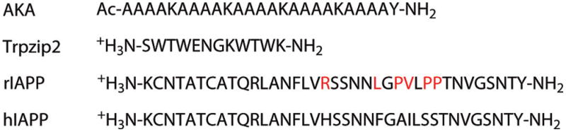
Sequences of peptides in this study: the AKA peptide, Trpzip2, rIAPP, and hIAPP. Different residues between rIAPP and hIAPP are shown in red in the rIAPP sequence. In both IAPP proteins, Cys2 and Cys7 are connected with disulfide bonds.

Figure 5.

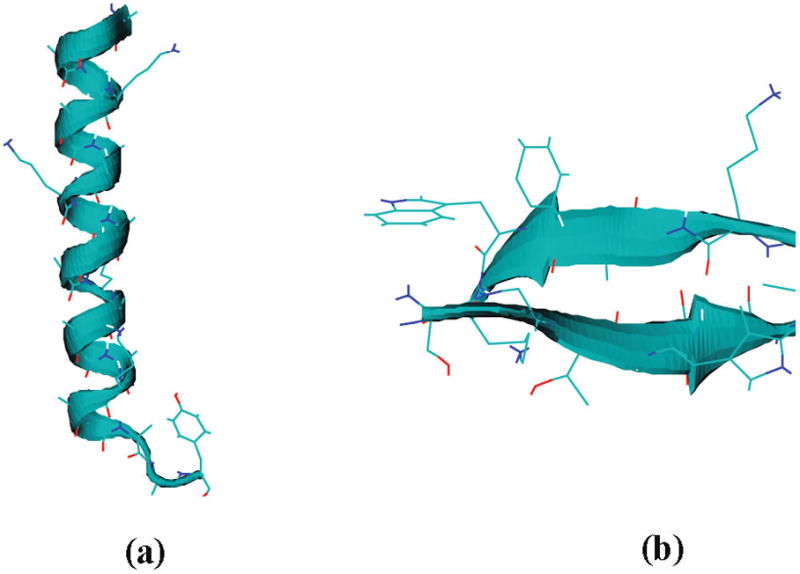
Representative snapshots of (a) AKA and (b) Trpzip2.

The initial structure of AKA was constructed by assuming a perfect α-helix with all (φ, ψ) angles set to (−57°, −47°). It was solvated in enough H₂O molecules to ensure a distance of 1 nm from all box edges. Side chains of lysines are positively charged, and chloride ions were added to neutralize them. The system was then energy-minimized and equilibrated with constant temperature for 20 ps with the positions of protein atoms frozen. Unconstrained simulations were then carried out to equilibrate the system, first in the NVT ensemble for 100 ps and then in the NpT ensemble for 5 ns. Properties such as temperature, pressure, density, and root-mean-square-deviations were monitored to ensure equilibration. An MD run for 10 ns was then performed at a time step of 2 fs. The LINCS algorithm was used to constrain all bonds, and PME was used to calculate the long-range Coulombic interactions. Berendsen coupling schemes for temperature and pressure¹⁴⁰ were used in the simulation. Temperature was set to be 275 K, in accordance with experiment.^30,32,87 The GROMACS source code was modified to report local frequencies on the fly using eqs 11 and 13. Frequencies and configurations were saved every 10 fs for spectra calculations. Throughout the 10 ns simulation, the central part of the peptide stays α-helical, while the C-terminus frays, as described in experimental studies.^{134,136,137,141}

Theoretical and experimental⁸⁷ spectra of unlabeled (but suitably deuterated) AKA peptide in D₂O are shown in Figure 6a. The theoretical spectrum peaks at 1627 cm⁻¹, differing from experiment by only 4 cm⁻¹. This peak position is determined by both the diagonal and off-diagonal elements of the Hamiltonian.¹⁴² On average, local frequencies of individual chromophores, at least in the central region of the helix (see below), are around 1640 cm⁻¹, which provides a central frequency that will be modified by couplings. Coupling constants between peptide units that are adjacent to each other (β₁₂), one residue apart (β₁₃), and two residues apart (β₁₄) have the largest magnitude and, thus, have the largest impact on the overall spectrum. β₁₂’s are positive for α-helices, as predicted by the NNC map and Ham et al.⁴⁷ The overall effect of positive β₁₂’s is a blue shift of the peak frequency. On the other hand, β₁₃, β₁₄, and other couplings between nonadjacent neighbors are negative, which counteract the effect of β₁₂ and lead to a final red shift of the peak position. The average β₁₂, β₁₃, and β₁₄ for residues 2–20 are shown in Table 4. Experimentally, coupling constants were extracted by systematically isotope-labeling two residues zero, one, and two residues apart.³⁰ Compared with experiment, the signs and relative magnitude of the three coupling constants are correct.

Figure 6.

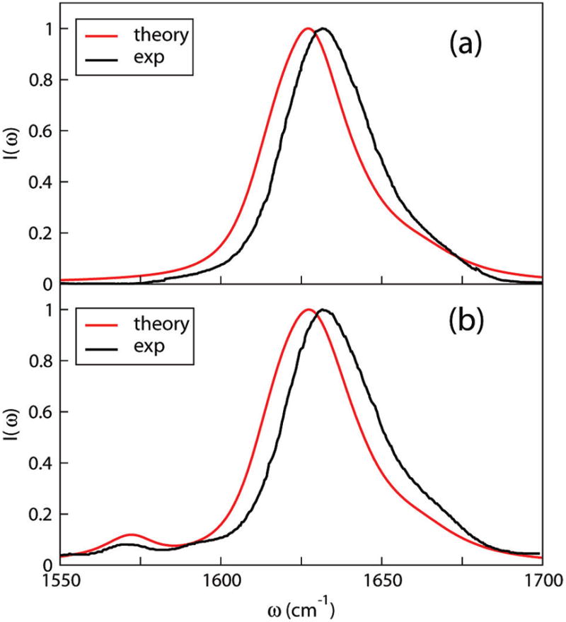
Theoretical and experimental IR absorption spectra of (a) unlabeled⁸⁷ and (b) [12] labeled³² AKA peptide.

Table 4.

Theoretical and Experimental³⁰ Coupling Constants for the AKA Peptide^a

	β12	β13	β14
theory	5.2 ± 0.3	−1.5 ± 0.2	−5.6 ± 0.2
experiment	8.5 ± 1.8	−5.4 ± 1.0	−6.6 ± 0.8

^aTheoretical values are averaged over residues 2–20. All coupling constants are in cm⁻¹.

We also carried out calculations on isotope-edited AKA peptides. The frequency shift of ¹³C=¹⁸O is assumed to be −70 cm⁻¹, consistent with previous experiments and ab initio calculations.^{27–29,32,47} One ¹³C=¹⁸O label was placed on residue 12 (denoted as [12]), and the full spectrum was calculated by shifting the frequency of the labeled residue and retaining all the couplings. This procedure was repeated for residues [13], [14], and [15]. All four spectra appear quite similar. The [12] spectrum is shown in Figure 6b along with the experimental result.³² Note the good agreement of the labeled features at about 1570 cm⁻¹. To compare further the isotope-labeled feature, we assume each residue is ¹³C=¹⁸O-labeled, one at a time, and treat each one of them as an isolated chromophore and neglect couplings. Isotope-labeled peak frequencies as a function of residue are shown in Figure 7. Peaks in the central region stay more or less constant, consistent with a homogeneous α-helical configuration. Experimental results³² for residues [12], [13], [14], and [15], which differ from theory by only a few cm⁻¹, confirm our combined electrostatic and NNFS⁶⁷ scheme for calculating backbone frequencies.

Figure 7.

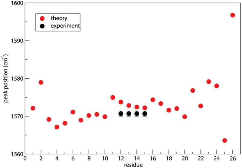
¹³C=¹⁸O labeled peak frequencies as a function of residue number for the AKA peptide. The theoretical isotope shift is taken to be −70 cm⁻¹. Experimental³² isotope-labeled peak frequencies are shown for residues 12–15.

C. β-Hairpin Model System: The Trpzip2 Peptide

Tryptophan zippers (Trpzips) are stable, monomeric β-hairpins in aqueous solution at room temperature.¹⁴³ Trpzip2 is one of the most stable molecules in the Trpzip family and has been extensively studied.^{70,71,88,89,144–146} The sequence and configuration of Trpzip2 are shown in Figures 4 and 5b. Amidated Trpzip2 contains 11 backbone chromophores, 1 “side-chain” chromophore at the C-terminus, and 1 side-chain chromophore on Asn6.

The initial configuration of Trpzip2 was taken from the Protein Data Bank (PDB ID 1LE1). MD simulations were run with procedures similar to those for AKA. The simulation temperature was 298 K. Theoretical and experimental⁸⁸ spectra are shown in Figure 8a, both of which have a two-peak feature. The two peaks are presumably due, in part, to collective motions of chromophores that give rise to a⁻ and a⁺ type peaks.^88,145–148 Agreement between theory and experiment, while not perfect, is still quite good (in that the theoretical positions and intensities of both peaks are about right).

Figure 8.

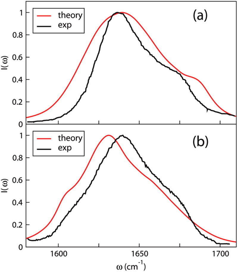
Theoretical and experimental⁸⁸ IR absorption spectra of (a) unlabeled, and (b) T3*– T10* labeled Trpzip2 in D₂O.

Apart from couplings, inhomogeneity of diagonal frequencies also contribute to the spectral features. Assuming that the ¹³C label shifts the frequency by −43 cm⁻¹,^26,34,47,89 and assuming that labeled chromophores are isolated, the labeled peak frequencies as a function of backbone residue number are plotted in Figure 9. The frequencies show a zigzag pattern due to alternating hydrogen-bonding environments, in agreement with previous simulation results.^70,145 Carbonyls facing inside the hairpin form a single intramolecular hydrogen bond, whereas carbonyls facing outside the hairpin form two hydrogen bonds with surrounding water molecules. Correspondingly, the latter have lower frequencies. The nondegenerate local frequencies fall into two regions, corresponding to the two peaks in the spectrum. ¹³C-labeling experiments^88,89 confirm this inhomogeneity because the frequencies of residues 3 and 10 are ~25 cm⁻¹ higher than that of residue 2, which is, in turn, 10 cm⁻¹ higher than the frequency of residue 7. These experimental frequencies are also shown in Figure 9. They are qualitatively in agreement with theory; the lack of quantitative agreement is most likely due (in part) to the fact that ¹³C-labeled residues are not fully localized, as was assumed in these particular theoretical calculations.

Figure 9.

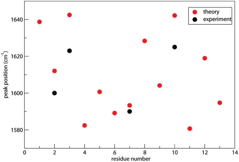
¹³C-labeled peak frequencies as a function of residue number for Trpzip2. Residue 13 is the side chain chromophore on Asn6. The theoretical isotope shift is taken to be −43 cm⁻¹. Also shown are experimental^88,89 isotope-labeled peak frequencies at residues 2, 3, 7, and 10.

Theoretical and experimental spectra of Trpzip2 doubly labeled by ¹³C at positions 3 and 10 (denoted as T3*–T10*) are shown in Figure 8b. In accordance with experiment,⁸⁸ the theoretical spectrum shows a less prominent shoulder around 1680 cm⁻¹, with a new shoulder appearing around 1605 cm⁻¹. The former is easy to understand, since the unlabeled local frequencies of residues 3 and 10 are both about 1680 cm⁻¹ (from the results in Figure 9 plus 43 cm⁻¹), when these residues are labeled the intensity near 1680 cm⁻¹ drops. When residues 3 and 10 are labeled, they mix with other lower-frequency residues, causing the theoretical shift of the main peak and appearance of the low-frequency shoulder.

The lack of quantitative agreement between theory and experiment for the Trpzip2 problem may result from our use of the TDC approximation for nearby chromophores interacting across the β-hairpin, which is questionable.¹⁴⁹

D. IAPP

Islet amyloid polypeptide (IAPP) is a 37-residue peptide. Amyloid fibrils of human IAPP (hIAPP) are a common pathological characteristic of type 2 diabetes.^150,151 The aggregation process and cell disruption mechanisms are not clear due to its fast aggregation kinetics. Rat IAPP (rIAPP), which differs from hIAPP at only 6 residues, does not form aggregates. The sequences of hIAPP and rIAPP are shown in Figure 4. Three proline mutations at positions 25, 28, and 29 are believed to prevent rIAPP from forming aggregates. Investigation of the monomer conformational states of both peptides in solution is a first step toward understanding the aggregation process. Note that rIAPP and hIAPP each have six Asn residues (each with a side-chain chromophore), one Gln residue with its side-chain chromophore, and an additional “side-chain” chromophore at the C-terminus as a result of amidation. For both peptides, Cys2 and Cys7 are connected by disulfide bonds.

Reddy et al. presented combined replica exchange umbrella sampling and MD simulations on rIAPP monomer.⁹⁰ Both “folded” and random-coil conformations were observed for rIAPP in aqueous solution, with relative populations of 55% and 45%, respectively.⁹⁰ Representative configurations of the two conformers are shown in Figure 10. Theoretical IR absorption spectra of rIAPP were presented previously⁹⁰ using the improved S2 map.⁵⁸ In the present paper, the same line shape calculations have been performed with the new frequency maps. The results of each conformer, weighted by their relative populations, and the total spectrum are shown in Figure 11. The theoretical spectrum is considerably improved compared with the previous result⁹⁰ and is in good agreement with experiment.⁹⁰ (Note that the slight disagreement with experiment around 1600 cm⁻¹ might be ameliorated with an improved map for proline because there are three such residues in rIAPP.) In part, the improvement between theory and experiment is due to the new side-chain map (rIAPP has eight side-chain chromophores); the previous calculation used a backbone map for all (including side-chain) chromophores. One notices that both conformers absorb at about 1645 cm⁻¹, and the random-coil conformer has a wider line width due to its flexibility. The similarity in spectral features is due to the similarity in the three-dimensional structures. The folded conformer has an α-helical segment consisting of only residues 7–17, with the remaining part being mainly random coil. The α-helical segment leads to a red shift of the spectrum, but because 70% of the structure is random coil, its spectroscopic feature is quite similar to the random-coil conformer.

Figure 10.

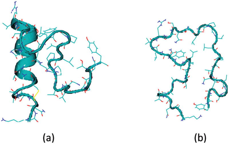
Representative snapshots of rIAPP monomer in (a) folded, and (b) random coil conformation.⁹⁰.

Figure 11.

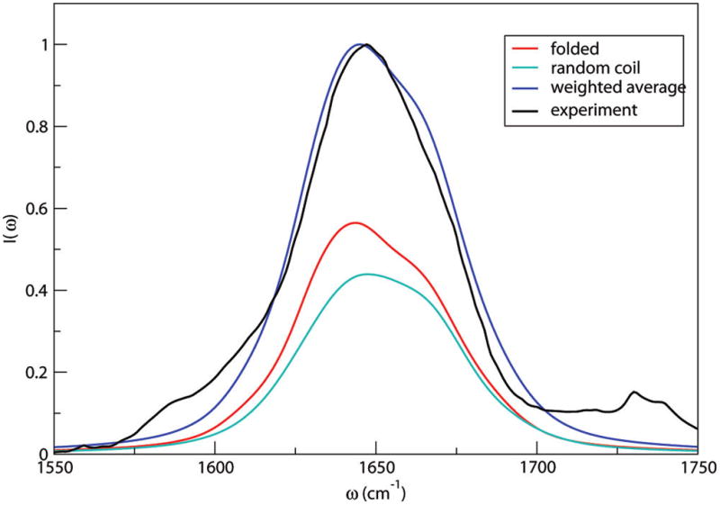
Theoretical (weighted average) and experimental⁹⁰ IR line shapes in the amide I stretch region of rIAPP in D₂O. Also shown are line shapes for the folded and random coil states, weighted by their relative probabilities.

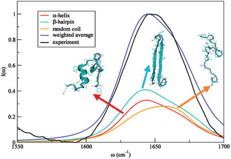
Following similar procedures, the hIAPP monomer is found to adopt α-helical, β-hairpin (“misfolded”), and random-coil conformations, with relative populations of 31%, 40%, and 29%, respectively.⁹¹ Representative snapshots along the simulations are shown in Figure 12. Theoretical and experimental spectra are shown in Figure 13.⁹¹ In this case, the α-helical and random-coil conformers have distinct spectral features. The α-helical conformer has residues 9–17 forming an α-helical structure, with a short antiparallel β-sheet at the C-terminus.^91,152 This more-ordered structure absorbs at 1644 cm⁻¹, 10 cm⁻¹ red-shifted compared with the random-coil conformer. The misfolded conformer has an antiparallel β-hairpin structure,^91,152 whose amide I peaks appear at 1642 and 1670 cm⁻¹. The total spectrum is in good agreement with experiment, suggesting the existence of the β-hairpin structure in the solution phase. The fiber of aggregated hIAPP molecules is composed of parallel β-sheet structures, and the misfolded conformer might be a precursor for aggregation.^91,152

Figure 12.

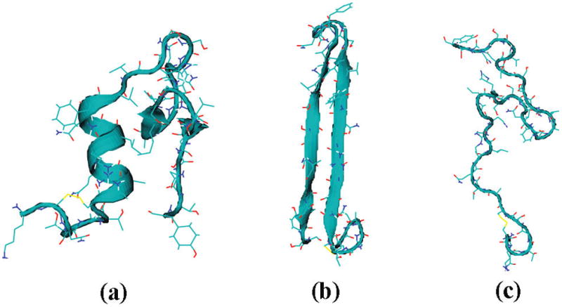
Representative snapshots of hIAPP monomer in (a) α-helical, (b) β-hairpin, and (c) random coil conformation.⁹¹

Figure 13.

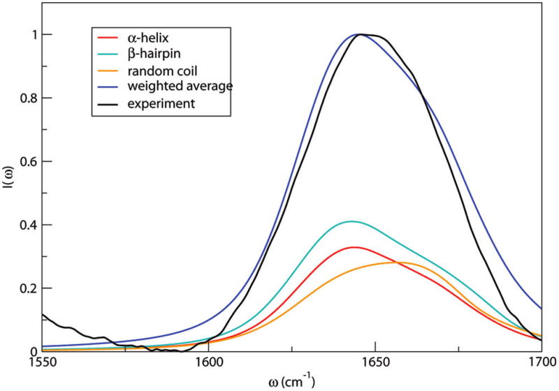
Theoretical (weighted average) and experimental⁹¹ IR line shapes in the amide I stretch region of hIAPP in D₂O. Also shown are line shapes for the α-helical, β-hairpin, and random coil states, weighted by their relative probabilities.

VI. CONCLUSIONS

In this paper, we have developed frequency maps for protein backbone and side chain amide I absorptions, from experimental line shapes and vibrational lifetimes on model compounds in different solvents. We have validated the maps by applying them, together with previously developed NNFS⁶⁷ and coupling maps,^42,67 to absorption spectra of model coupounds with a pair of chromophores, and unlabeled and (isotope)-labeled peptides with well-defined α-helical and β-hairpin secondary structures. Our theoretical results are in very good agreement with experiment, without any ad hoc frequency shifts or further adjustments (typical discrepancies between theory and experiment are on the order of a few wavenumbers). The fact that the frequency maps, applied with the GROMOS96 53a6 force field, are able to capture key features in the experimental spectra for a variety of different systems provides a way to bridge computer simulations and IR experiments. As computer power increases, simulations for large proteins for biologically relevant time scales will soon be possible. This and other theoretical frameworks that can accurately and efficiently calculate IR spectra, combined with experimental approaches, will enable the understanding of protein structure and dynamics at the molecular level.

The advancement of 2DIR opens a wide area for applications of these maps. 2DIR, with its superior time and frequency resolution, has become a powerful tool for probing protein structure and dynamics.^{20–25,37,153} The frequency maps can thus be utilized to study protein folding, hydrogen-bonding dynamics, protein aggregation, and so forth in aqueous solutions. Moreover, because the maps are designed (by considering different solvents) to be transferable, they are potentially applicable to more heterogeneous, including hydrophobic, environments. One possible application is the study of protein structure and dynamics in the presence of membranes. Membrane peptides are usually hard to crystallize and, thus, remain challenging for techniques such as X-ray crystallography, whereas IR spectroscopy can be utilized to study structure and in situ kinetics. We are carrying out further studies to validate the frequency maps using 2DIR experiments both in the presence and absence of lipid membranes.

For example, our ability to reproduce experimental absorption spectra of rIAPP and hIAPP monomers in solution is promising. 2DIR experiments, coupled with ¹³C=¹⁸O isotope labeling techniques, have been applied to the aggregation study of hIAPP in aqueous solution and in lipid vesicles.^37,153 It has been widely accepted that the aggregation process of hIAPP is greatly accelerated in the presence of lipid membranes.^154–156 In turn, intermediates along the aggregation pathway disrupt the membrane structure and possibly lead to cell death.^157–160 Line shape calculations, combined with extensive computer simulations, can provide details on oligomer and aggregate formation and explain changes of spectroscopic features observed in experiment along the aggregation pathway, which may shed light on the aggregation mechanism and, ultimately, on the medical treatment of type 2 diabetes.

References

- 1.Dickerson RE, Geis I. The structure and action of proteins. W. A. Benjamin, Inc; Menlo Park, CA: 1969. [Google Scholar]
- 2.Nelson DL, Cox MM. Lehninger Principles of Biochemistry. W. H. Freeman and Company; New York: 2005. [Google Scholar]
- 3.Berg JM, Tymoczko JL, Stryer L. Biochemistry. W. H. Freeman and Company; New York: 2007. [Google Scholar]
- 4.McCammon JA, Harvey SC. Dynamics of Proteins and Nucleic Acids. Cambridge University Press; Cambridge: 1987. [Google Scholar]
- 5.Boehr DD, Dyson HJ, Wright PE. Chem Rev. 2006;106:3055. doi: 10.1021/cr050312q. [DOI] [PubMed] [Google Scholar]
- 6.Kraut J. Annu Rev Biochem. 1965;34:247. doi: 10.1146/annurev.bi.34.070165.001335. [DOI] [PubMed] [Google Scholar]
- 7.Cartailler J-P, Luecke H. Annu Rev Biophys Biomol Struct. 2003;32:285. doi: 10.1146/annurev.biophys.32.110601.142516. [DOI] [PubMed] [Google Scholar]
- 8.Clore GM, Gronenborn AM, editors. NMR of Proteins. CRC Press Inc; Boca Raton, FL: 1993. [Google Scholar]
- 9.Thomas GJ., Jr Annu Rev Biophys Biomol Struct. 1999;28:1. doi: 10.1146/annurev.biophys.28.1.1. [DOI] [PubMed] [Google Scholar]
- 10.Kelly SM, Price NC. Biochim Biophys Acta. 1997;1338:161. doi: 10.1016/s0167-4838(96)00190-2. [DOI] [PubMed] [Google Scholar]
- 11.Margittai M, Langen R. Q Rev Biophys. 2008;41:265. doi: 10.1017/S0033583508004733. [DOI] [PubMed] [Google Scholar]
- 12.Weng L, Baker GM. Biochemistry. 1991;30:5727. doi: 10.1021/bi00237a014. [DOI] [PubMed] [Google Scholar]
- 13.Yan Y, Marriott G. Curr Opin Chem Biol. 2003;7:635. doi: 10.1016/j.cbpa.2003.08.017. [DOI] [PubMed] [Google Scholar]
- 14.Krimm S, Bandekar J. Adv Protein Chem. 1986;38:181. doi: 10.1016/s0065-3233(08)60528-8. [DOI] [PubMed] [Google Scholar]
- 15.Barth A, Zscherp C. Q Rev Biophys. 2002;35:369. doi: 10.1017/s0033583502003815. [DOI] [PubMed] [Google Scholar]
- 16.Susi H, Byler DM. Methods Enzymol. 1986;130:290. doi: 10.1016/0076-6879(86)30015-6. [DOI] [PubMed] [Google Scholar]
- 17.Haris PI, Chapman D. Trends Biochem Sci. 1992;17:328. doi: 10.1016/0968-0004(92)90305-s. [DOI] [PubMed] [Google Scholar]
- 18.Surewicz WK, Mantsch HH, Chapman D. Biochemistry. 1993;32:389. doi: 10.1021/bi00053a001. [DOI] [PubMed] [Google Scholar]
- 19.Hamm P, Lim M, Hochstrasser RM. J Phys Chem B. 1998;102:6123. [Google Scholar]
- 20.Zanni MT, Hochstrasser RM. Curr Opin Struct Biol. 2001;11:516. doi: 10.1016/s0959-440x(00)00243-8. [DOI] [PubMed] [Google Scholar]
- 21.Hochstrasser RM. Proc Natl Acad Sci USA. 2007;104:14190. doi: 10.1073/pnas.0704079104. [DOI] [PMC free article] [PubMed] [Google Scholar]
- 22.Park S, Kwak K, Fayer MD. Laser Phys Lett. 2007;4:704. [Google Scholar]
- 23.Cho M. Chem Rev. 2008;108:1331. doi: 10.1021/cr078377b. [DOI] [PubMed] [Google Scholar]
- 24.Ganim Z, Chung HS, Smith AW, DeFlores LP, Jones KC, Tokmakoff A. Acc Chem Res. 2008;41:432. doi: 10.1021/ar700188n. [DOI] [PubMed] [Google Scholar]
- 25.Strasfeld DB, Ling YL, Shim S-H, Zanni MT. J Am Chem Soc. 2008;130:6698. doi: 10.1021/ja801483n. [DOI] [PMC free article] [PubMed] [Google Scholar]
- 26.Tadesse L, Nazarbaghi R, Walters L. J Am Chem Soc. 1991;113:7036. [Google Scholar]
- 27.Torres J, Adams PD, Arkin IT. J Mol Biol. 2000;300:677. doi: 10.1006/jmbi.2000.3885. [DOI] [PubMed] [Google Scholar]
- 28.Torres J, Kukol A, Goodman JM, Arkin IT. Biopolymers. 2001;59:396. doi: 10.1002/1097-0282(200111)59:6<396::AID-BIP1044>3.0.CO;2-Y. [DOI] [PubMed] [Google Scholar]
- 29.Fang C, Wang J, Charnley AK, Barber-Armstrong W, Smith AB, Decatur SM, Hochstrasser RM. Chem Phys Lett. 2003;382:586. [Google Scholar]
- 30.Fang C, Wang J, Kim YS, Charnley AK, Barber-Armstrong W, Smith AB, Decatur SM, Hochstrasser RM. J Phys Chem B. 2004;108:10415. [Google Scholar]
- 31.Mukherjee P, Krummel AT, Fulmer EC, Kass I, Arkin IT, Zanni MT. J Chem Phys. 2004;120:10215. doi: 10.1063/1.1718332. [DOI] [PubMed] [Google Scholar]
- 32.Fang C, Hochstrasser RM. J Phys Chem B. 2005;109:18652. doi: 10.1021/jp052525p. [DOI] [PubMed] [Google Scholar]
- 33.Arkin IT. Curr Opin Chem Biol. 2006;10:394. doi: 10.1016/j.cbpa.2006.08.013. [DOI] [PMC free article] [PubMed] [Google Scholar]
- 34.Decatur SM. Acc Chem Res. 2006;39:169. doi: 10.1021/ar050135f. [DOI] [PubMed] [Google Scholar]
- 35.Mukherjee P, Kass I, Arkin I, Zanni MT. Proc Natl Acad Sci USA. 2006;103:3528. doi: 10.1073/pnas.0508833103. [DOI] [PMC free article] [PubMed] [Google Scholar]
- 36.Mukherjee P, Kass I, Arkin IT, Zanni MT. J Phys Chem B. 2006;110:24740. doi: 10.1021/jp0640530. [DOI] [PMC free article] [PubMed] [Google Scholar]
- 37.Shim S-H, Gupta R, Ling YL, Strasfeld DB, Raleigh DP, Zanni MT. Proc Natl Acad Sci USA. 2009;106:6614. doi: 10.1073/pnas.0805957106. [DOI] [PMC free article] [PubMed] [Google Scholar]
- 38.Strasfeld DB, Ling YL, Gupta R, Raleigh DP, Zanni MT. J Phys Chem B. 2009;113:15679. doi: 10.1021/jp9072203. [DOI] [PMC free article] [PubMed] [Google Scholar]
- 39.Manor J, Mukherjee P, Lin Y-S, Leonov H, Skinner JL, Zanni MT, Arkin IT. Structure. 2009;17:247. doi: 10.1016/j.str.2008.12.015. [DOI] [PMC free article] [PubMed] [Google Scholar]
- 40.Woys AM, Lin Y-S, Reddy AS, Xiong W, de Pablo JJ, Skinner JL, Zanni MT. J Am Chem Soc. 2010;132:2832. doi: 10.1021/ja9101776. [DOI] [PubMed] [Google Scholar]
- 41.Torii H, Tasumi M. J Chem Phys. 1992;96:3379. [Google Scholar]
- 42.Torii H, Tasumi M. J Raman Spectrosc. 1998;29:81. [Google Scholar]
- 43.Torii H. J Phys Chem B. 2007;111:5434. doi: 10.1021/jp070301w. [DOI] [PubMed] [Google Scholar]
- 44.Torii H. Mol Phys. 2009;107:1855. [Google Scholar]
- 45.Hamm P, Woutersen S. Bull Chem Soc Jpn. 2002;75:985. [Google Scholar]
- 46.Ham S, Kim J-H, Lee H, Cho M. J Chem Phys. 2003;118:3491. [Google Scholar]
- 47.Ham S, Cha S, Choi J-H, Cho M. J Chem Phys. 2003;119:1451. [Google Scholar]
- 48.Ham S, Cho M. J Chem Phys. 2003;118:6915. [Google Scholar]
- 49.Kwac K, Cho M. J Chem Phys. 2003;119:2247. [Google Scholar]
- 50.Choi J-H, Ham S, Cho M. J Phys Chem B. 2003;107:9132. [Google Scholar]
- 51.Hahn S, Ham S, Cho M. J Phys Chem B. 2005;109:11789. doi: 10.1021/jp050450j. [DOI] [PubMed] [Google Scholar]
- 52.Choi J-H, Hahn S, Cho M. Int J Quantum Chem. 2005;104:616. [Google Scholar]
- 53.Choi J-H, Lee H, Lee K-K, Hahn S, Cho M. J Chem Phys. 2007;126:045102. doi: 10.1063/1.2424711. [DOI] [PubMed] [Google Scholar]
- 54.Jeon J, Yang S, Choi J-H, Cho M. Acc Chem Res. 2009;42:1280. doi: 10.1021/ar900014e. [DOI] [PubMed] [Google Scholar]
- 55.Bouř P, Keiderling T. J Chem Phys. 2003;119:11253. [Google Scholar]
- 56.Bouř P, Michalík D, Kapitán J. J Chem Phys. 2005;122:144501. doi: 10.1063/1.1877272. [DOI] [PubMed] [Google Scholar]
- 57.Schmidt JR, Corcelli SA, Skinner JL. J Chem Phys. 2004;121:8887. doi: 10.1063/1.1791632. [DOI] [PubMed] [Google Scholar]
- 58.Lin Y-S, Shorb JM, Mukherjee P, Zanni MT, Skinner JL. J Phys Chem B. 2009;113:592. doi: 10.1021/jp807528q. [DOI] [PMC free article] [PubMed] [Google Scholar]
- 59.Hochstrasser RM. Adv Chem Phys. 2006;132:1. [Google Scholar]
- 60.Hayashi T, Zhuang W, Mukamel S. J Phys Chem A. 2005;109:9747. doi: 10.1021/jp052324l. [DOI] [PubMed] [Google Scholar]
- 61.Zhuang W, Abramavicius D, Hayashi T, Mukamel S. J Phys Chem B. 2006;110:3362. doi: 10.1021/jp055813u. [DOI] [PMC free article] [PubMed] [Google Scholar]
- 62.Sengupta N, Maekawa H, Zhuang W, Toniolo C, Mukamel S, Tobias DJ, Ge N-H. J Phys Chem B. 2009;113:12037. doi: 10.1021/jp901504r. [DOI] [PMC free article] [PubMed] [Google Scholar]
- 63.Zhuang W, Hayashi T, Mukamel S. Angew Chem, Int Ed. 2009;48:3750. doi: 10.1002/anie.200802644. [DOI] [PMC free article] [PubMed] [Google Scholar]
- 64.Maekawa H, Ge N-H. J Phys Chem B. 2010;114:1434. doi: 10.1021/jp908695g. [DOI] [PubMed] [Google Scholar]
- 65.Ganim Z, Tokmakoff A. Biophys J. 2006;91:2636. doi: 10.1529/biophysj.106.088070. [DOI] [PMC free article] [PubMed] [Google Scholar]
- 66.Watson TM, Hirst JD. Mol Phys. 2005;103:1531. [Google Scholar]
- 67.la Cour Jansen T, Dijkstra AG, Watson TM, Hirst JD, Knoester J. J Chem Phys. 2006;125:044312. doi: 10.1063/1.2218516. [DOI] [PubMed] [Google Scholar]
- 68.la Cour Jansen T, Knoester J. J Chem Phys. 2006;124:044502. doi: 10.1063/1.2148409. [DOI] [PubMed] [Google Scholar]
- 69.Bloem R, Dijkstra AG, la Cour Jansen T, Knoester J. J Chem Phys. 2008;129:055101. doi: 10.1063/1.2961020. [DOI] [PubMed] [Google Scholar]
- 70.Roy S, la Cour Jansen T, Knoester J. Phys Chem Chem Phys. 2010;12:9347. doi: 10.1039/b925645h. [DOI] [PubMed] [Google Scholar]
- 71.Smith AW, Lessing J, Ganim Z, Peng CS, Tokmakoff A, Roy S, la Cour Jansen T, Knoester J. J Phys Chem B. 2010;114:10913. doi: 10.1021/jp104017h. [DOI] [PubMed] [Google Scholar]
- 72.Gorbunov RD, Kosov DS, Stock G. J Chem Phys. 2005;122:224904. doi: 10.1063/1.1898215. [DOI] [PubMed] [Google Scholar]
- 73.Gorbunov RD, Nguyen PH, Kobus M, Stock G. J Chem Phys. 2007;126:054509. doi: 10.1063/1.2431803. [DOI] [PubMed] [Google Scholar]
- 74.Gorbunov RD, Stock G. Chem Phys Lett. 2007;437:272. [Google Scholar]
- 75.Kobus M, Gorbunov RD, Nguyen PH, Stock G. Chem Phys. 2008;347:208. [Google Scholar]
- 76.Cai K, Han C, Wang J. Phys Chem Chem Phys. 2009;11:9149. doi: 10.1039/b910269h. [DOI] [PubMed] [Google Scholar]
- 77.Paschek D, Pühse M, Perez-Goicochea A, Gnanakaran S, Garcia AE, Winter R, Geiger A. ChemPhysChem. 2008;9:2742. doi: 10.1002/cphc.200800540. [DOI] [PubMed] [Google Scholar]
- 78.Kim J, Huang R, Kubelka J, Bouř P, Keiderling TA. J Phys Chem B. 2006;110:23590. doi: 10.1021/jp0640575. [DOI] [PubMed] [Google Scholar]
- 79.Grahnen JA, Amunson KE, Kubelka J. J Phys Chem B. 2010;114:13011. doi: 10.1021/jp106639s. [DOI] [PubMed] [Google Scholar]
- 80.Zhao J, Wang J. J Phys Chem B. 2010;114:16011. doi: 10.1021/jp108324p. [DOI] [PubMed] [Google Scholar]
- 81.Choi J-H, Cho M. J Chem Phys. 2004;120:4383. doi: 10.1063/1.1644100. [DOI] [PubMed] [Google Scholar]
- 82.Choi J-H, Cho M. Chem Phys. 2009;361:168. [Google Scholar]
- 83.Krimm S, Abe Y. Proc Natl Acad Sci USA. 1972;69:2788. doi: 10.1073/pnas.69.10.2788. [DOI] [PMC free article] [PubMed] [Google Scholar]
- 84.Moore WH, Krimm S. Proc Natl Acad Sci USA. 1975;72:4933. doi: 10.1073/pnas.72.12.4933. [DOI] [PMC free article] [PubMed] [Google Scholar]
- 85.Cheam TC, Krimm S. Chem Phys Lett. 1984;107:613. [Google Scholar]
- 86.Cheam TC, Krimm S. J Chem Phys. 1985;82:1631. [Google Scholar]
- 87.Barber-Armstrong W, Donaldson T, Wijesooriya H, Silva RAGD, Decatur SM. J Am Chem Soc. 2004;126:2339. doi: 10.1021/ja037863n. [DOI] [PubMed] [Google Scholar]
- 88.Smith AW, Tokmakoff A. J Chem Phys. 2007;126:045109. doi: 10.1063/1.2428300. [DOI] [PubMed] [Google Scholar]
- 89.Wang J, Chen J, Hochstrasser RM. J Phys Chem B. 2006;110:7545. doi: 10.1021/jp057564f. [DOI] [PMC free article] [PubMed] [Google Scholar]
- 90.Reddy AS, Wang L, Lin Y-S, Ling Y, Chopra M, Zanni MT, Skinner JL, de Pablo JJ. Biophys J. 2010;98:443. doi: 10.1016/j.bpj.2009.10.029. [DOI] [PMC free article] [PubMed] [Google Scholar]
- 91.Reddy AS, Wang L, Singh S, Ling YL, Buchanan L, Zanni MT, Skinner JL, de Pablo JJ. Biophys J. 2010;99:2208. doi: 10.1016/j.bpj.2010.07.014. [DOI] [PMC free article] [PubMed] [Google Scholar]
- 92.McQuarrie DA. Statistical Mechanics. Harper and Row; New York: 1976. [Google Scholar]
- 93.Auer BM, Skinner JL. J Chem Phys. 2007;127:104105. doi: 10.1063/1.2766943. [DOI] [PubMed] [Google Scholar]
- 94.Auer BM, Skinner JL. J Chem Phys. 2008;128:224511. doi: 10.1063/1.2925258. [DOI] [PubMed] [Google Scholar]
- 95.Mukamel S. Principles of Nonlinear Optical Spectroscopy. Oxford; New York: 1995. [Google Scholar]
- 96.Schmidt JR, Corcelli SA, Skinner JL. J Chem Phys. 2005;123:044513. doi: 10.1063/1.1961472. [DOI] [PubMed] [Google Scholar]
- 97.DeCamp MF, DeFlores L, McCracken JM, Tokmakoff A, Kwac K, Cho M. J Phys Chem B. 2005;109:11016. doi: 10.1021/jp050257p. [DOI] [PubMed] [Google Scholar]
- 98.Shim S-H, Strasfeld DB, Zanni MT. Opt Express. 2006;14:13120. doi: 10.1364/oe.14.013120. [DOI] [PubMed] [Google Scholar]
- 99.Shim S-H, Strasfeld DB, Fulmer EC, Zanni MT. Opt Lett. 2006;31:838. doi: 10.1364/ol.31.000838. [DOI] [PubMed] [Google Scholar]
- 100.van Gunsteren WF, Billeter SR, Eising AA, Hünenberger PH, Krüger P, Mark AE, Scott WRP, Tironi IG. Biomolecular Simulation: The GROMOS96 manual and user guide. Hochschuleverlag AG an der ETH Zürich; Zürich, Switzerland: 1996. [Google Scholar]
- 101.Scott WRP, Hünenberger PH, Tironi IG, Mark AE, Billeter SR, Fennen J, Torda AE, Huber T, Krüger P, van Gunsteren WF. J Phys Chem A. 1999;103:3596. [Google Scholar]
- 102.Oostenbrink C, Villa A, Mark AE, van Gunsteren WF. J Comput Chem. 2004;25:1656. doi: 10.1002/jcc.20090. [DOI] [PubMed] [Google Scholar]
- 103.Zagrovic B, van Gunsteren WF. Proteins. 2006;63:210. doi: 10.1002/prot.20872. [DOI] [PubMed] [Google Scholar]
- 104.Zhou Y, Oostenbrink C, Jongejan A, van Gunsteren WF, Hagen WR, de Leeuw SW, Jongejan JA. J Comput Chem. 2006;27:857. doi: 10.1002/jcc.20378. [DOI] [PubMed] [Google Scholar]
- 105.Bekker H, Berendsen HJC, Dijkstra EJ, Achterop S, van Drunen R, van der Spoel D, Sijbers A, Keegstra H, Reitsma B, Renardus MKR. In: Physics Computing ‘92. de Groot RA, Nadrchal J, editors. World Scientific; Singapore: 1993. [Google Scholar]
- 106.Berendsen HJC, van der Spoel D, van Drunen R. Comput Phys Commun. 1995;91:43. [Google Scholar]
- 107.Lindahl E, Hess B, van der Spoel D. J Mol Model. 2001;7:306. [Google Scholar]
- 108.van der Spoel D, Lindahl E, Hess B, van Buuren AR, Apol E, Meulenhoff PJ, Tieleman DP, Sijbers ALTM, Feenstra KA, van Drunen R, Berendsen HJC. Gromacs User Manual version 33. 2005 www.gromacs.org.
- 109.van der Spoel D, Lindahl E, Hess B, Groenhof G, Mark AE, Berendsen HJC. J Comput Chem. 2005;26:1701. doi: 10.1002/jcc.20291. [DOI] [PubMed] [Google Scholar]
- 110.Hess B, Bekker H, Berendsen HJC, Fraaije JGEM. J Comput Chem. 1997;18:1463. [Google Scholar]
- 111.Ryckaert J-P, Ciccotti G, Berendsen HJC. J Comput Phys. 1977;23:327. [Google Scholar]
- 112.Darden T, York D, Pedersen L. J Chem Phys. 1993;98:10089. [Google Scholar]
- 113.Essmann U, Perera L, Berkowitz ML, Darden T, Lee H, Pedersen LG. J Chem Phys. 1995;103:8577. [Google Scholar]
- 114.Press WH, Flannery BP, Teukolsky SA, Vetterling WT. Numerical Recipes. Cambridge University Press; Cambridge: 1986. [Google Scholar]
- 115.Mayne LC, Hudson B. J Phys Chem. 1991;95:2962. [Google Scholar]
- 116.Eaton G, Symons MCR, Rastogi PP. J Chem Soc, Faraday Trans 1. 1989;85:3257. [Google Scholar]
- 117.Kubelka J, Keiderling TA. J Phys Chem A. 2001;105:10922. [Google Scholar]
- 118.Nyquist RA. Spectrochim Acta. 1963;19:509. [Google Scholar]
- 119.Davies M, Hallam HE. Trans Faraday Soc. 1951;47:1170. [Google Scholar]
- 120.Brown TL, Regan JF, Schuetz RD, Sternberg JC. J Phys Chem. 1959;63:1324. [Google Scholar]
- 121.Titov EV, Poddubnaya MV, Kapkan LM. Theor Exp Chem. 1973;6:421. [Google Scholar]
- 122.Ruggirello A, Liveri VT. Colloid Polym Sci. 2003;281:1062. [Google Scholar]
- 123.Amunson KE, Kubelka J. J Phys Chem B. 2007;111:9993. doi: 10.1021/jp072454p. [DOI] [PubMed] [Google Scholar]
- 124.Berendsen HJC, Postma JPM, van Gunsteren WF, Hermans J. In: Intermolecular Forces. Pullman B, editor. Reidel; Dordrecht: 1981. [Google Scholar]
- 125.Chirgadze YN, Fedorov OV, Trushina NP. Biopolymers. 1975;14:679. doi: 10.1002/bip.1975.360140402. [DOI] [PubMed] [Google Scholar]
- 126.Venyaminov SY, Kalnin NN. Biopolymers. 1990;30:1243. doi: 10.1002/bip.360301309. [DOI] [PubMed] [Google Scholar]
- 127.Rahmelow K, Hübner W, Ackermann T. Anal Biochem. 1998;257:1. doi: 10.1006/abio.1997.2502. [DOI] [PubMed] [Google Scholar]
- 128.Barth A. Prog Biophys Mol Biol. 2000;74:141. doi: 10.1016/s0079-6107(00)00021-3. [DOI] [PubMed] [Google Scholar]
- 129.Wolpert M, Hellwig P. Spectrochim Acta, Part A. 2006;64:987. doi: 10.1016/j.saa.2005.08.025. [DOI] [PubMed] [Google Scholar]
- 130.Barth A. Biochim Biophys Acta. 2007;1767:1073. doi: 10.1016/j.bbabio.2007.06.004. [DOI] [PubMed] [Google Scholar]
- 131.la Cour Jansen T, Knoester J. J Phys Chem B. 2006;110:22910. doi: 10.1021/jp064795t. [DOI] [PubMed] [Google Scholar]
- 132.Yang M, Skinner JL. Phys Chem Chem Phys. 2010;12:982. doi: 10.1039/b918314k. [DOI] [PubMed] [Google Scholar]
- 133.Marqusee S, Robbins VH, Baldwin RL. Proc Natl Acad Sci USA. 1989;86:5286. doi: 10.1073/pnas.86.14.5286. [DOI] [PMC free article] [PubMed] [Google Scholar]
- 134.Miick SM, Casteel KM, Millhauser GL. Biochemistry. 1993;32:8014. doi: 10.1021/bi00082a024. [DOI] [PubMed] [Google Scholar]
- 135.Fiori WR, Miick SM, Millhauser GL. Biochemistry. 1993;32:11957. doi: 10.1021/bi00096a003. [DOI] [PubMed] [Google Scholar]
- 136.Decatur SM, Antonic J. J Am Chem Soc. 1999;121:11914. [Google Scholar]
- 137.Decatur SM. Biopolymers. 2000;54:180. doi: 10.1002/1097-0282(200009)54:3<180::AID-BIP40>3.0.CO;2-9. [DOI] [PubMed] [Google Scholar]
- 138.Silva RAGD, Nguyen JY, Decatur SM. Biochemistry. 2002;41:15296. doi: 10.1021/bi026507z. [DOI] [PubMed] [Google Scholar]
- 139.Huang R, Kubelka J, Barber-Armstrong W, Silva RAGD, Decatur SM, Keiderling TA. J Am Chem Soc. 2004;126:2346. doi: 10.1021/ja037998t. [DOI] [PubMed] [Google Scholar]
- 140.Berendsen HJC, Postma JPM, van Gunsteren WF, DiNola A, Haak JR. J Chem Phys. 1984;81:3684. [Google Scholar]
- 141.Silva RAGD, Kubelka J, Bou P, Decatur SM, Keiderling TA. Proc Natl Acad Sci USA. 2000;97:8318. doi: 10.1073/pnas.140161997. [DOI] [PMC free article] [PubMed] [Google Scholar]
- 142.Hamm P, Zanni MT. Concepts and Methods in 2D IR Spectroscopy. Cambridge University Press; Cambridge, UK: 2011. [Google Scholar]
- 143.Cochran AG, Skelton NJ, Starovasnik MA. Proc Natl Acad Sci USA. 2001;98:5578. doi: 10.1073/pnas.091100898. [DOI] [PMC free article] [PubMed] [Google Scholar]
- 144.Smith AW, Chung HS, Ganim Z, Tokmakoff A. J Phys Chem B. 2005;109:17025. doi: 10.1021/jp053949m. [DOI] [PubMed] [Google Scholar]
- 145.Wang J, Zhuang W, Mukamel S, Hochstrasser RM. J Phys Chem B. 2008;112:5930. doi: 10.1021/jp075683k. [DOI] [PMC free article] [PubMed] [Google Scholar]
- 146.la Cour Jansen T, Knoester J. Biophys J. 2008;94:1818. doi: 10.1529/biophysj.107.118851. [DOI] [PMC free article] [PubMed] [Google Scholar]
- 147.Cheatum CM, Tokmakoff A, Knoester J. J Chem Phys. 2004;120:8201. doi: 10.1063/1.1689637. [DOI] [PubMed] [Google Scholar]
- 148.Dijkstra AG, Knoester J. J Phys Chem B. 2005;109:9787. doi: 10.1021/jp044141p. [DOI] [PubMed] [Google Scholar]
- 149.Moran A, Mukamel S. Proc Natl Acad Sci USA. 2004;101:506. doi: 10.1073/pnas.2533089100. [DOI] [PMC free article] [PubMed] [Google Scholar]
- 150.Clark A, Cooper GJS, Lewis CE, Morris JF, Willis AC, Reid KBM, Turner RC. The Lancet. 1987;2:231. doi: 10.1016/s0140-6736(87)90825-7. [DOI] [PubMed] [Google Scholar]
- 151.Lorenzo A, Razzaboni B, Weir GC, Yankner BA. Nature. 1994;368:756. doi: 10.1038/368756a0. [DOI] [PubMed] [Google Scholar]
- 152.Dupuis NF, Wu C, Shea J-E, Bowers MT. J Am Chem Soc. 2009;131:18283. doi: 10.1021/ja903814q. [DOI] [PMC free article] [PubMed] [Google Scholar]
- 153.Ling YL, Strasfeld DB, Shim S-H, Raleigh DP, Zanni MT. J Phys Chem B. 2009;113:2498. doi: 10.1021/jp810261x. [DOI] [PMC free article] [PubMed] [Google Scholar]
- 154.Knight JD, Miranker AD. J Mol Biol. 2004;341:1175. doi: 10.1016/j.jmb.2004.06.086. [DOI] [PubMed] [Google Scholar]
- 155.Jayasinghe SA, Langen R. Biochemistry. 2005;44:12113. doi: 10.1021/bi050840w. [DOI] [PubMed] [Google Scholar]
- 156.Knight JD, Hebda JA, Miranker AD. Biochemistry. 2006;45:9496. doi: 10.1021/bi060579z. [DOI] [PubMed] [Google Scholar]
- 157.Jayasinghe SA, Langen R. Biochim Biophys Acta. 2007;1768:2002. doi: 10.1016/j.bbamem.2007.01.022. [DOI] [PubMed] [Google Scholar]
- 158.Brender JR, Lee EL, Cavitt MA, Gafni A, Steel DG, Ramamoorthy A. J Am Chem Soc. 2008;130:6424. doi: 10.1021/ja710484d. [DOI] [PMC free article] [PubMed] [Google Scholar]
- 159.Engel MFM, Khemtémourian L, Kleijer CC, Meeldijk HJD, Jacobs J, Verkleij AJ, de Kruijff B, Killian JA, Höppener JWM. Proc Natl Acad Sci USA. 2008;105:6033. doi: 10.1073/pnas.0708354105. [DOI] [PMC free article] [PubMed] [Google Scholar]
- 160.Smith PES, Brender JR, Ramamoorthy A. J Am Chem Soc. 2009;131:4470. doi: 10.1021/ja809002a. [DOI] [PMC free article] [PubMed] [Google Scholar]