Point-Process Analysis of Neural Spiking Activity of Muscle Spindles Recorded from Thin-Film Longitudinal Intrafascicular Electrodes

Abstract

Recordings from thin-film Longitudinal Intra-Fascicular Electrodes (tfLIFE) together with a wavelet-based de-noising and a correlation-based spike sorting algorithm, give access to firing patterns of muscle spindle afferents. In this study we use a point process probability structure to assess mechanical stimulus-response characteristics of muscle spindle spike trains. We assume that the stimulus intensity is primarily a linear combination of the spontaneous firing rate, the muscle extension, and the stretch velocity.

By using the ability of the point process framework to provide an objective goodness of fit analysis, we were able to distinguish two classes of spike clusters with different statistical structure. We found that spike clusters with higher SNR have a temporal structure that can be fitted by an inverse Gaussian distribution while lower SNR clusters follow a Poisson-like distribution. The point process algorithm is further able to provide the instantaneous intensity function associated with the stimulus-response model with the best goodness of fit.

This important result is a first step towards a point process decoding algorithm to estimate the muscle length and possibly provide closed loop Functional Electrical Stimulation (FES) systems with natural sensory feedback information.

I. INTRODUCTION

Functional electrical stimulation (FES) is a technique to restore motor function in people affected by spinal cord injury or other neurological disorders by using electrical currents to stimulate peripheral nerves and muscles distal to the lesion.

In order to increase stimulation functional efficacy and reduce fatigue, closed loop control FES is highly desirable but this requires reliable sensory information about the ongoing motor task. With the recent advances in interfacing with the peripheral nervous system [1], it is becoming possible to record afferent information coming from natural sensors located distally to the lesion and provide feedback to the controller [2], [3].

Muscle spindles are one type of such natural sensors. They lie in parallel with the extrafusal skeletal muscle fibers and detect changes in the length of the muscle. As these changes are associated with changes in the angles of the joints that the muscles cross, afferent neural activity from muscle spindle fibers can be used as feedback for controlling the position of the ankle joint [4].

Two groups of sensory fibers originate from muscle spindles: group Ia and group II. The former type of fibers encode information about both the rate of change and the absolute muscle length, while the latter predominantly encode information about the muscle length. A recent study explored the feasibility of estimating muscle length during passive stretch using a model-based interpretation of the nerve responses from muscle spindle afferents [5].

In the work presented here, we use a stimulus-response point process model [6], [7] to analyze the neural spiking activity of muscle spindles recorded from peripheral nerve interfaces.

II. METHODS

A. Experimental Setup

1) Animal Preparation

Experimental work was conducted on a 3.6 kg New Zealand white rabbit under a protocol approved by the Animal Experiment Inspectorate under the Danish Ministry of Justice. A detailed description of the setup appears in [8]. Briefly, the animal was anaesthetised using a Rompun cocktail (Ketamine 50 mg/mL, Xylazine 2.5 mg/mL, Acepromazine 0.5 mg/mL) dosed at 0.625 mL/kg. Once anaesthetised, surgical access to the sciatic and common peroneal nerves was created at the popliteal fossa. Fascicles of the sciatic nerve to the medial gastrocnemius and the lateral gastrocnemius/soleus muscles were identified and implanted with third generation thin film Longitudinal Intra-Fascicular Electrodes (tfLIFE3). The nerve was crushed proximal to the tfLIFE implantation site to remove the fusimotor drive to the intra-fusal fibers. Steinmann pins were placed at the distal epiphyses of the left femur and tibia and anchored to a rigid experimental frame. A second access was created just above the calcaneal tendon to expose the tendon and tie the tendon to a servocontrolled muscle puller (Aurora Scientific, 310B) set to the controlled position mode.

2) Data Acquisition

The experimental protocol and setup are described in detail previously [8]. Briefly, the amplification system consisted of a low-noise pre-amplifier (AI402, Axon Instruments), followed by a gain-filter amplifier (Cyberamp 380, Axon Instruments). Signals were recorded using a custom modified multi-channel digital tape recorder (ADAT-XT, Alesis). ENG data were band-pass filtered (4th order Bessel, corners at 0.1 Hz and 10 kHz), amplified (gain 5000) and acquired with a sampling rate of 48 kHz per channel.

3) Experimental Protocol

The muscle was presented with a random stretch profile. The ankle motion trajectory was synthesized by low-pass filtering a 3-minute long white noise sequence using a second-order Butterworth digital filter with 0.5 Hz cut-off. After filtering, the trajectory was scaled to produce muscle length variation within a peak to peak range of 4 mm. Force and position were recorded together with the neural signals. The muscle was not stimulated while being stretched.

B. De-noising and Spike Sorting

The recorded neural signals were wavelet-de-noised and spike-sorted using an approach based on [9].

Wavelet de-noising is a technique that can be used to attempt to remove noise from signals, e.g., neural recordings [10], and consists in three steps: transposing the noisy signals into an orthogonal time-scale domain, applying a threshold to the resulting coefficients, and finally transforming back into the original time domain. In this work a 5-level time-invariant wavelet decomposition scheme using the Symmlet 7 mother wavelet was adopted because of its similarity to typical action potentials waveforms. Hard-thresholding was used with level-dependent thresholds equal to 3 times the standard deviation (estimated using the median absolute deviation) of the corresponding wavelet coefficients at each level of decomposition. The approximation was completely discarded because it contained components below approximately 750 Hz.

The de-noised signal was later processed by an automated spike sorting algorithm in order to attempt to isolate single-unit action potential. We used a correlation-based sorting algorithm consisting of two phases. During the first phase a set of spike clusters was created. During the second phase the spikes in the signal were compared to each cluster template and labelled as belonging to its best match.

C. Point-Process model

1) Framework

Let (0, T] denote the observation interval and 0 ≤ u₁ < … < u_k < u_k+1 < … < u_K ≤ T the times of the events, ideally spikes. Here the times correspond to the matching of the recorded neural signal with a given cluster template. For t ∈ (0, T], let N(t) = max{k: u_k ≤ t} be the sample path of the associated counting process. For t ∈ (0, T], we define the conditional intensity function:

$${\lambda }_t(t)=\underset{\mathrm{\Delta }t\to 0}{lim}\frac{Pr(N(t+\mathrm{\Delta }t)-N(t)=1)}{\mathrm{\Delta }t}.$$ (1)

It follows from the theory of point processes [6] that the log-likelihood of observing the sample path N(t) or, equivalently, the sequence of events {u_k}, is:

$$\text{L}(N_{0:T})=\underset{0}{\overset{T}{\int }}log(\lambda (t))\text{d}N(t)+\underset{0}{\overset{T}{\int }}\lambda (t)\text{d}t.$$ (2)

Let f_z(z) be a renewal process probability density defined for z ∈ (0, ∞) which captures the ISI probability density under constant stimulus. Be λ_z(z) the associated conditional intensity (or hazard-rate) function:

$${\lambda }_z(z)=\frac{f(z)}{1-\underset{0}{\overset{z}{\int }}f(\zeta )\text{d}\zeta }.$$ (3)

Let g(t) be an intensity-rescaling transformation [7]

$$z=g(t)=\underset{u_{N(t^{-})}}{\overset{t}{\int }}s(\tau )\text{d}\tau$$ (4)

where s(t) is a strictly positive stimulus intensity function that accounts for the stimulus at each time t. By a change of variable, the conditional intensity function (1) can be written as:

$${\lambda }_t(t)=\frac{f_t(t)}{1-\underset{u_{N(t^{-})}}{\overset{t}{\int }}{f}_t(\tau )\text{d}\tau }=\frac{\frac{\text{d}g}{\text{d}t}{f}_z(g(t))}{1-\underset{0}{\overset{g(t)}{\int }}{f}_z(\zeta )\text{d}\zeta }=s(t){\lambda }_z(z).$$ (5)

2) Renewal Process Probability Density

An inverse Gaussian (IG) distribution has been assumed as renewal process probability density:

$$f_z(z)=f_{IG}(z)=\sqrt{\frac{k}{2\pi z^3}}exp\frac{-k}{2z}{\left(\frac{z}{\mu }-1\right)}^2.$$ (6)

This choice was made assuming that the sensory fiber can be modelled as an integrate-and-fire oscillator with fixed positive threshold driven by a Wiener process with positive drift whose distribution of ISIs is, in fact, inverse Gaussian [11].

The conditional intensity function of the inverse Gaussian distribution is

$${\lambda }_{IG}(z)=\frac{{\alpha }_3{f}_G({\alpha }_1-{\alpha }_2)}{1-(F_G({\alpha }_2-{\alpha }_1)+{\text{e}}^{2{\alpha }_1{\alpha }_2}{F}_G({\alpha }_1+{\alpha }_2))}$$ (7)

where $\alpha =[-\sqrt{kz}/\mu ,-\sqrt{k/z},\sqrt{k/z^3}]$ while f_G(x) and F_G(x) are the probability density function and the cumulative distribution function of a standard Gaussian distribution. Using the conditional intensity function of the IG distribution, λ_z(z) = λ_IG(z) in (5), with a z from (4), we obtain a model following an inhomogeneous inverse Gaussian (iIG) distribution. We also tested the alternative hypothesis that the renewal process probability follows an inhomogeneous Poisson (iP) distribution with conditional intensity function λ_z(z) = λ_P(z) = λ₀.

3) Stimulus Intensity Function

The stimulus intensity function s(t) was designed in order to incorporate the previous knowledge about the firing rate of muscle spindles. Both group Ia and group II fibres show an approximately linear relation between firing rate and muscle extension, as well as between firing rate and muscle extension velocity [12], [13]. Therefore we assumed that the stimulus intensity is a linear combination of the spontaneous firing rate, the muscle extension, and the stretch velocity. As in some conditions (e.g., the descending ramp of a stretch-hold-release sequence) the fiber can stop firing completely, we used a saturation function log(e^x + 1) that approaches the identity function for x → +∞ and converges to 0 for x → −∞. The resulting stimulus intensity function was

$$s(t)=log\left[exp\left({\beta }_0+{\beta }_{e}l(t)+{\beta }_v\frac{\text{d}l(t)}{\text{d}t}\right)+1\right]$$ (8)

where l(t) is the muscle extension.

As this stimulus intensity function already incorporates a spontaneous firing activity through β₀, we set the location parameter of the renewal process to one, i.e., μ = 1 and λ₀ = 1.

By forcing β_e = 0 and β_v = 0, we also tested the alternative hypothesis that the probability distributions of the ISIs are homogeneous (hIG and hP), i.e., they do not depend on the input.

4) Model Fitting

After sampling the point process (N(t)) and the input (l(t)) at 1 ms steps, the likelihood function (2) was evaluated as a finite sum of the contributions at each sample. Thanks to the fact that (5), (7), (8) and the sampled version of (2) are differentiable with respect to the parameters and available in closed form, it is possible to find the derivatives of L(N_0:T) with respect to the vector of model parameters θ = [k, β₀, β_e, β_v] and apply the Newton-Raphson method to find the set of parameters maximizing the likelihood.

We used the time-rescaling theorem to construct Kolmogorov-Smirnov goodness-of-fit tests for the fitted models. The results can be visually represented by means of K-S plots which provide a graphical summary for comparing the model fits with the data [6].

III. RESULTS

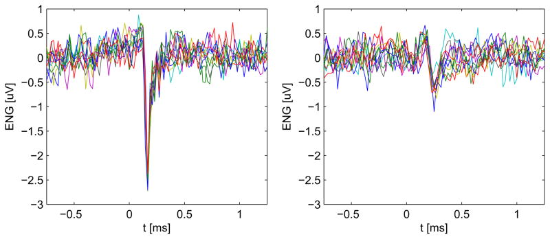
Within the 180 s recording, the spike sorting algorithm found 9 distinct spike clusters. Figure 1 shows an example of two of the spike clusters found, one with high signal to noise ratio (SNR) and one with lower SNR. The SNR was defined as the ratio between the peak amplitude of the cluster spike template and the square root of the background noise variance.

Fig. 1.

Ten randomly selected occurrences of the spike cluster 4 (left) and ten of the spike cluster 8 (right). The amplitude of the spikes is well above the noise level for cluster 4 while it is slightly above the noise level for cluster 8, resulting in a lower SNR.

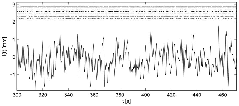
Figure 2 shows a raster plot for the 9 clusters together with the input signal (the muscle extension, l(t)).

Fig. 2.

Plot of the input signal l(t), i.e., the muscle extension. In the upper part, a raster plot for the 9 clusters starting from cluster 1 (top).

We fitted the spike train corresponding to each one of the spike clusters, to the four distributions (iIG, hIG, iP, hP) described before. The results are summarized in Table I.

TABLE I.

Fitted Models

Cluster	spikes	SNR	fit	k	β0	βe	βv
1	1612	3.01	hP,iP	–	7.97	−0.696	0.23
2	1633	3.10	hP,iP	–	8.22	0.151	0.171
3	380	11.0	hIG,iIG	0.888	−5.57	7.80	4.60
4	521	12.5	iIG	1.23	−3.88	9.13	5.41
5	1482	3.32	iP	–	7.40	3.08	1.87
6	399	3.75	hP,iP	–	−2.66	2.17	0.485
7	857	3.14	hP,iP	–	2.39	0.491	0.500
8	413	3.58	hP,iP	–	−2.65	3.05	1.33
9	604	3.87	hP,iP	–	−0.247	3.36	1.74

Fitting of the spike train of each spike cluster to the four distributions (iIG, hIG, iP, hP). For each spike cluster we report: (a) the number of spikes (column 2); (b) the SNR (column 3); (c) which ones of the four models pass the K-S test, i.e., the corresponding K-S plot lies within the acceptance bounds (column 4); and (d) the parameters of the inhomogeneous model passing the K-S test (columns 5 to 8).

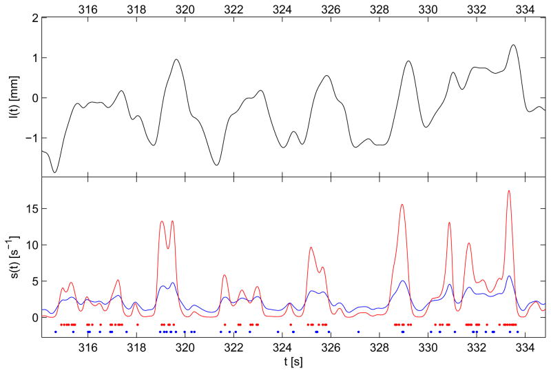
Figure 3 shows a few seconds of the input l(t) and the stimulus intensity function s(t) for spike clusters 4 and 8 together with their raster plots.

Fig. 3.

The upper plot shows a few seconds of the muscle extension l(t). The lower plot presents the stimulus intensity function s(t) and the raster plot of the spike clusters 4 (red) and 8 (blue). The stimulus intensity function has been evaluated substituting the corresponding parameters from Table I in (8).

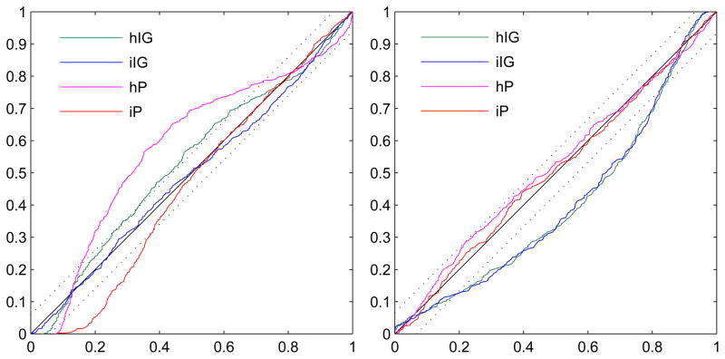
Figure 4 shows the K-S plots related to the two spike clusters presented before. For cluster 4, the K-S plot of the inhomogeneous inverse Gaussian distribution lies within the confidence bounds, meaning that it is able to capture both the time structure of the ISIs and their dependence on the input l(t). On the contrary, for cluster 8, it is the inhomogeneous Poisson that fits the data best while the iIG is well outside the confidence bounds.

Fig. 4.

K-S plots of the four models for the spike clusters 4 (left) and 8 (right). For cluster 4, neither the homogeneous nor the inhomogeneous Poisson distributions fit the data adequately. The homogeneous inverse Gaussian provides a better fit but still outside the confidence bounds. On the contrary, the inhomogeneous inverse Gaussian presents a very good fit of the data meaning that it captures both the time structure of the ISIs and their dependence on the input. Cluster 8 shows a specular situation where the two inverse Gaussian distributions fail to fit the data while both the two Poisson distributions are within the confidence bounds, with the inhomogeneous Poisson being slightly closer to the 45°line.

It is worth noting that the clusters associated to the spike trains for which the iIG is acceptable are those with higher SNR, while those for which the iP model fits the spike train best have a much lower SNR. A possible explanation is that those clusters with higher SNR are probably able to selectively identify the action potential that propagates along a single axon close to the electrode. Therefore their temporal structure is closer to the theoretical model of an integrate-and-fire neuron.

On the contrary, clusters matching lower SNR spikes are less selective and are likely to capture action potentials from a higher number of distant axons. Therefore the resulting spike trains could represent the combined activity of several sensory fibers. In this case the resulting point process sample path N(t) would be the sum of many independent point process paths. Even for non-Poisson statistics, e.g. IG, of the single spike train, the resulting sum follows an exponential ISI distribution like a Poisson process (even though it is not a Poisson process [14]). Another reason for the ISI of low SNR spikes for being closer to a Poisson distribution is that, as their amplitude is closer to the noise level, the resulting spike trains might be polluted by noise spikes for which it is reasonable to assume a Poisson distribution.

IV. CONCLUSIONS

We have presented a point process framework to model the afferent muscle spindle activity recorded from tfLIFEs inserted in the sciatic nerve of a rabbit.

Results report high goodness of fit and provide relevant insights into the statistical properties of the fiber response to both stretch and velocity. This novel study is a first important step towards a point process decoding algorithm to estimate the muscle length and possibly provide closed loop Functional Electrical Stimulation (FES) systems with natural sensory feedback information.

References

- 1.Navarro X, Krueger TB, Lago N, Micera S, Stieglitz T, Dario P. A critical review of interfaces with the peripheral nervous system for the control of neuroprostheses and hybrid bionic systems. J Peripher Nerv Syst. 2005 Sept;10(3):229–258. doi: 10.1111/j.1085-9489.2005.10303.x. [DOI] [PubMed] [Google Scholar]
- 2.Hoffer JA, Stein RB, Haugland MK, Sinkjaer T, Durfee WK, Schwartz AB, Loeb GE, Kantor C. Neural signals for command control and feedback in functional neuromuscular stimulation: a review. J Rehabil Res Dev. 1996 Apr;33(2):145–157. [PubMed] [Google Scholar]
- 3.Haugland M, Hoffer J, Sinkjaer T. Skin contact force information in sensory nerve signals recorded by implanted cuff electrodes. IEEE Trans Rehabil Eng. 1994;2(1):18–28. [Google Scholar]
- 4.Yoshida K, Horch K. Closed-loop control of ankle position using muscle afferent feedback with functional neuromuscular stimulation. IEEE Trans Biomed Eng. 1996 Feb;43(2):167–176. doi: 10.1109/10.481986. [DOI] [PubMed] [Google Scholar]
- 5.Djilas M, Azevedo-Coste C, Guiraud D, Yoshida K. Interpretation of muscle spindle afferent nerve response to passive muscle stretch recorded with thin-film longitudinal intrafascicular electrodes. IEEE Trans Neural Syst Rehabil Eng. 2009 Oct;17(5):445–453. doi: 10.1109/TNSRE.2009.2032286. [DOI] [PubMed] [Google Scholar]
- 6.Brown EN, Barbieri R, Eden UT, Frank LM. Likelihood methods for neural spike train data analysis. In: Feng J, editor. Computational Neuroscience: A Comprehensive Approach. Chapman and Hall/CRC; 2003. pp. 253–286. [Google Scholar]
- 7.Barbieri R, Quirk MC, Frank LM, Wilson MA, Brown EN. Construction and analysis of non-poisson stimulus-response models of neural spiking activity. J Neurosci Methods. 2001 Jan;105(1):25–37. doi: 10.1016/s0165-0270(00)00344-7. [DOI] [PubMed] [Google Scholar]
- 8.Djilas M, Azevedo-Coste C, Guiraud D, Yoshida K. Spike sorting of muscle spindle afferent nerve activity recorded with thin-film intrafascicular electrodes. Comput Intell Neurosci. 2010:836346. doi: 10.1155/2010/836346. [DOI] [PMC free article] [PubMed] [Google Scholar]
- 9.Citi L, Carpaneto J, Yoshida K, Hoffmann KP, Koch KP, Dario P, Micera S. On the use of wavelet denoising and spike sorting techniques to process electroneurographic signals recorded using intraneural electrodes. J Neurosci Methods. 2008 July;172(2):294–302. doi: 10.1016/j.jneumeth.2008.04.025. [DOI] [PubMed] [Google Scholar]
- 10.Diedrich A, Charoensuk W, Brychta RJ, Ertl AC, Shiavi R. Analysis of raw microneurographic recordings based on wavelet de-noising technique and classification algorithm: wavelet analysis in microneurography. IEEE Trans Biomed Eng. 2003 Jan;50(1):41–50. doi: 10.1109/TBME.2002.807323. [DOI] [PMC free article] [PubMed] [Google Scholar]
- 11.Paninski L, Brown EN, Iyengar S, Kass RE. Statistical models of spike trains. In: Laing C, Lord G, editors. Stochastic Methods in Neuroscience. Oxford University Press; 2008. [Google Scholar]
- 12.Harvey RJ, Matthews PB. The response of de-efferented muscle spindle endings in the cat’s soleus to slow extension of the muscle. J Physiol. 1961 July;157:370–392. doi: 10.1113/jphysiol.1961.sp006729. [DOI] [PMC free article] [PubMed] [Google Scholar]
- 13.Matthews PB. The response of de-efferented muscle spindle receptors to stretching at different velocities. J Physiol. 1963 Oct;168:660–678. doi: 10.1113/jphysiol.1963.sp007214. [DOI] [PMC free article] [PubMed] [Google Scholar]
- 14.Lindner B. Superposition of many independent spike trains is generally not a poisson process. Phys Rev E Stat Nonlin Soft Matter Phys. 2006 Feb;73(2 Pt 1):022901. doi: 10.1103/PhysRevE.73.022901. [DOI] [PubMed] [Google Scholar]