Automated detection of mass lesions in dedicated breast CT: A preliminary study

Abstract

Purpose: To develop an automated method to detect breast masses on dedicated breast CT (BCT) volumes and to conduct a preliminary evaluation of its performance. This method can be used in a computer-aided detection (CADe) system for noncontrast enhanced BCT.

Methods: The database included patient images, which were acquired under an IRB-approved protocol. The database in this study consisted of 132 cases. 50 cases contained 58 malignant masses, and 23 cases contained 24 benign masses. 59 cases did not contain any biopsy-proven lesions. Each case consisted of an unenhanced CT volume of a single breast. First, each breast was segmented into adipose and glandular tissues using a fuzzy c-means clustering algorithm. The glandular breast regions were then sampled at a resolution of 2 mm. At each sampling step, a 3.5-cm³ volume-of-interest was subjected to constrained region segmentation and 17 characteristic features were extracted, yielding 17 corresponding feature volumes. Four features were selected using step-wise feature selection and merged with linear discriminant analysis trained in the task of distinguishing between normal breast glandular regions and masses. Detection performance was measured using free-response receiver operating characteristic analysis (FROC) with leave-one-case-out evaluation.

Results: The feature selection stage selected features that characterized the shape and margin strength of the segmented region. CADe sensitivity per case was 84% (std = 4.2%) at 2.6 (std = 0.06) false positives per volume, or 6 × 10⁻³ per slice (at an average of 424 slices per volume in this data set).

Conclusions: This preliminary study demonstrates the feasibility of our approach for CADe for BCT.

INTRODUCTION

Mammography is the current gold standard for breast cancer screening, contributing an estimated 46% to the reduction in breast cancer mortality between 1975 and 2000.¹ Despite this success, a major limitation of mammography is tissue superimposition caused by the projection of a complex 3D structure onto a planar detector. Tissue superimposition can obscure or mimic lesions, which potentially reduces both sensitivity and specificity of mammography.²

To overcome this limitation, dedicated breast CT (BCT) is being developed^{3, 4, 5, 6} to produce a 3D CT volume data set of the breast at the same dose as two mammographic projection views. In the BCT image, the breast structure is fully resolved in three dimensions at a resolution of 200–400 μm. Two clinical studies have compared lesion conspicuity in BCT and mammography.^{4, 5} In both contrast-enhanced and nonenhanced BCT, conspicuity of mass lesions was greater in BCT than it was in mammography. The conspicuity of lesions was further improved with the administration of intravenous contrast.

With BCT the amount of data that the radiologist needs to review for each breast is increased substantially. To support the radiologists’ management of this data volume, an algorithm to automatically detect mass lesions in BCT has been developed. In BCT, where the number of images per case is increased 200 fold, the demands on the radiologist to remain vigilant during interpretation are increased. In this circumstance, computer-aided detection (CADe) may play an important role in reducing radiologists’ miss rate and reading fatigue. Several studies have shown that computer-aided detection in mammography screening can improve detection sensitivity,^{7, 8, 9, 10, 11, 12} albeit with an increase in recall rate.

To the best of our knowledge, we report here the first CADe scheme developed for BCT. CADe schemes for digital breast tomosynthesis, which is a quasi-3D x-ray breast-imaging modality, are being developed.^{13, 14, 15} We describe our CADe scheme for BCT and its preliminary performance results in this study.

METHODS

Image dataset

In this HIPAA-compliant study, patient images were acquired following IRB protocol. Patients that had received a BIRADS score of 4 or 5 based on diagnostic breast-imaging workup and had given informed consent were imaged by BCT prior to biopsy. Patient selection criteria are detailed in Appendix B. Patient ages ranged between 37 and 82 years with a mean of 55.6 years. All scans used in this study were unenhanced.

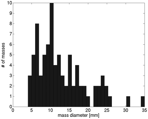
All images were acquired on the Albion dedicated breast CT prototype unit developed at the University of California at Davis.⁵ Pixels in the coronal BCT plane were square and varied between 190 and 390 μm. Along the direction perpendicular to the coronal plane (i.e., slice spacing,) voxel dimension varied between 200 and 770 μm. Lesion centers were identified by an experienced research technician and verified by a radiologist, and lesion diameter d_mass was the largest dimension of the mass lesion in the coronal plane. The distribution of mass diameters is shown in Fig. 1.

Figure 1.

Distribution of mass diameters in the dataset.

Each case consisted of the unenhanced breast CT volume of a single breast. The data set contained 132 cases: 50 cases contained 58 malignant masses, 23 cases contained 24 benign biopsy-proven lesions, and 59 normal cases contained no biopsy-proven lesions. Normal cases were BCT scans of the contralateral breasts that had no abnormalities. The number of cases in the four BI-RADS breast density categories¹⁶ were 5 (3.8%), 59 (44.7%), 55 (41.7%), 13 (9.8%).

Preprocessing: Identification of gland tissue

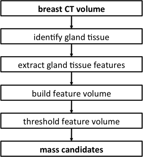
A flowchart describing the automated mass detection scheme is shown in Fig. 2. The first step in the algorithm was to identify the breast region, and the adipose and glandular tissue regions within the breast. A gray-value threshold of − 400 Hounsfield units (HU) was used to identify the breast region. Holes in the breast region were filled using the matlab “imfill” function¹⁷ and the breast volume was eroded with a cube-shaped structuring element (side length = 3 mm) to remove skin. Note that the aim of this preprocessing step was to remove the skin region from subsequent analysis, rather than to generate a detailed outline of the skin. The breast region was filtered with a cubic 3³ voxel averaging filter to reduce image noise.

Figure 2.

Algorithm flowchart.

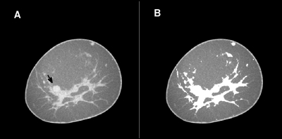
Next, the adipose and glandular tissue regions in the breast volume were identified using a fuzzy c-means based segmentation scheme. The glandular tissue class could include high-contrast objects such as calcifications. Fuzzy c-means segmentation has been used previously in breast MRI.¹⁸ The tissue segmentation was performed slice-by-slice in the coronal slices of the breast volume. First, a 3rd order polynomial surface fit to voxels with HU < − 100 was subtracted from the coronal slice to reduce nonuniformity in the coronal slice due to incomplete scatter correction. Next, fuzzy c-means clustering was performed with four classes. The regions with the lowest and second lowest class prototypes were labeled adipose, and the region with the highest class prototype was labeled glandular. If the difference between the intermediate class prototypes (2nd and 3rd highest prototype) was above 30 HU, the region corresponding to the second-highest class prototype was labeled glandular, otherwise adipose. An example of this tissue segmentation is shown in Fig. 3.

Figure 3.

A coronal slice through a BCT volume (A). The same coronal slice, but with pixels classified as glandular tissue set to “white” (B). Note that this BCT slice contains a malignant lesion, which is shown with the computer outline in Fig. 4.

Extraction of gland tissue features

Next, a Cartesian grid (with isotropic sampling distance of 2 mm) was placed over the breast volume. Grid points located within glandular tissue were considered seed points around which a cubic volume-of-interest (VOI) with 3.5-cm side length was extracted. Each VOI was submitted to constrained radial gradient index (RGI) region segmentation.¹⁹ The RGI for a region margin dΩ is given by

$$\mathrm{RGI}=\frac{{\displaystyle \sum _{d\Omega }}\overrightarrow{G}(\overrightarrow{r})·\hat{r}(\overrightarrow{r})}{{\displaystyle \sum _{d\Omega }}|\overrightarrow{G}(\overrightarrow{r})|},$$ (1)

where $\overrightarrow{r}=(x,y,z)$ is a location along dΩ and $\overrightarrow{G}(\overrightarrow{r})$ is the image gradient at location $\overrightarrow{r}$.

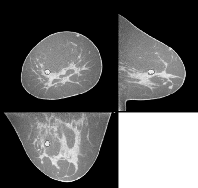
Initially, to constrain the segmented region, the VOI is initially multiplied with a 3D Gaussian (σ = 1 cm). Then, a set of 3D regions is generated by thresholding this processed VOI over a range of threshold values. The RGI is computed for each region margin using the original VOI data. The actual segmentation is the region for which RGI is highest. An example of a segmented lesion is shown in Fig. 4. For each breast CT volume, the volumetric glandular fraction was determined as the ratio of glandular tissue volume to breast volume. Skin was excluded.

Figure 4.

Example of a malignant lesion that was detected by the algorithm, shown in the coronal, axial and sagittal slices centered on the lesion. The outline of the RGI segmentation is overlaid in red. This same case was also shown in Fig. 3.

From each segmented region, 17 characteristic features were extracted, including morphologic, gradient, histogram and texture features. The features and their definitions are listed in Appendix A.

Classifier training

The purpose of the classifier was to distinguish seed points that are located in normal gland tissue, from seed points that are located within a lesion. For feature selection and classifier training, each VOI seed point was labeled as “normal” or “mass” based on the seed point’s distance to an actual lesion center, which had been identified by the radiologist. Since segmentation accuracy decreased with increasing seed point distance from the lesion center, features extracted for seed points far from the lesion center (but still within the lesion) characterize a lesion less accurately. Therefore, seed points labeled “mass” were required to be located within 2.5 mm of the lesion center regardless of the actual lesion size.

The resulting training data were highly unbalanced, i.e., the number of true data samples (mass) was by a factor of ∼800 lower than the number of false data samples (normal glandular tissue). Because linear discriminant analysis (LDA) performs suboptimally if the training data are unbalanced, a training set with equal prevalence was constructed by replicating the true data samples, following Xue and Titterington.²⁰

A subset of four features was selected using step-wise feature selection,²¹ which were merged using a LDA classifier trained to distinguish actual lesion VOIs from normal glandular tissue VOIs. Classifier training and testing was performed using a leave-one-case-out scheme: All cases except one were used to select four features and train the LDA classifier, and the remaining case, with all of its VOIs, was used as a test case to measure algorithm performance. This was iterated over the entire data set so that each case was used as a test case once, and average sensitivity and false positive rate was determined.

Extraction of mass candidates

Features extracted along the seed point grid within each BCT volume yielded “feature volumes”. For example, a “margin strength” volume resulted from the calculation of the margin strength feature at each seed point along the grid at which a successful segmentation was obtained. The four feature volumes (for each of the four features selected in the linear stepwise feature selection step) were merged by computing the linear discriminant distance $\lambda (\overrightarrow{r})$ at each seed point $\overrightarrow{r}$

$$\lambda (\overrightarrow{r})={\overrightarrow{\omega }}_{\mathrm{LDA}}·\overrightarrow{f}(\overrightarrow{r}),$$ (2)

where ${\overrightarrow{\omega }}_{\mathrm{LDA}}$ contains the LDA weights and $\overrightarrow{f}(\overrightarrow{r})$ is a vector containing four features.

A final merged feature volume was generated from λ, subject to the following rules: (1) region size greater than 27 mm³ and (2) contrast greater than 90 HU or less than 180 HU. Note that contrast is the difference between the average CT number in the segmented region and adjacent adipose tissue, which is expected to be of this order.

The merged feature volume can be viewed as a “probability map” in which higher values corresponded to a greater likelihood that a lesion is present.²² From the merged feature volume, mass candidates were extracted at a threshold, which was chosen so that a preset number of mass candidates were allowed per case (T = target number of detections). Each mass candidate location corresponded to the centroid of a region that (1) exceeded the gray-value threshold and (2) consisted of at least three 18-connected voxels.

Scoring a “true-positive detection” required that the mass candidate center be located within a sphere of diameter d = d_mass around the actual mass center. Otherwise, the mass candidate was scored as a false positive detection. A free-response receiver operating characteristic (FROC) curve was generated by varying T, the target number of detections. Algorithm sensitivity and false positives per BCT volume were estimated using a leave-one-case-out technique over classifier training. The results of the leave-one-case-out training and testing were bootstrapped to estimate variability from choice of test cases. Table Table I. summarizes the algorithm parameters used in this study.

Table 1.

Algorithm parameters.

Noise reduction	33 voxels averaging filter
Seed point sampling distance	2 mm
Constraint function	Gaussian, σ = 1 cm
Minimum region size	(3 mm)3
Minimum region contrast	90 HU
Maximum region contrast	180 HU
Number of features extracted	17
Number of features selected	4
Region connectivity	18

RESULTS

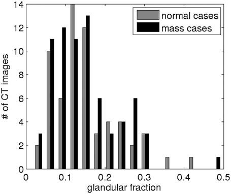
The distribution of volumetric glandular fractions of all breast CT volumes in this study is shown in Fig. 5.

Figure 5.

Volumetric glandular fraction of the breast CT volumes.

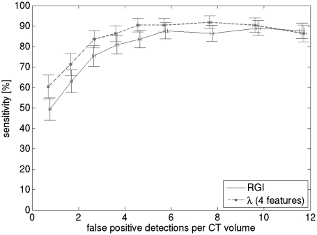
FROC performance of the CADe algorithm is shown in Fig. 6; performance of the dominant RGI feature is also shown. CADe sensitivity was 84% (std = 4.2%) at 2.6 (std = 0.06) false positives per BCT volume. At each iteration of the leave-one-case-out scheme, the feature set was noted. The feature set, which was automatically determined using linear step-wise feature selection within the leave-one-case-out scheme, did not vary and included relative RGI, irregularity, contrast, and ellipsoid semi-axes minimum to maximum ratio.

Figure 6.

FROC performance of the RGI feature, as well as the complete CADe algorithm with four features. CADe sensitivity is per case, and was estimated using a leave-one-case-out scheme. The length of the error bars is two standard deviations, estimated from 1000 bootstrap samples. Three features indicates that feature selection and LDA classifier training was performed using all lesions as training data, four features indicates that the training data consisted of malignant lesions only.

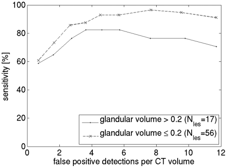
The effect of breast density on CADe performance is shown in Fig. 7. The BCT cases were divided into two groups, with glandular fraction below or above 0.2, which is the average glandular fraction.²³ The graphs indicate, as expected, that algorithm performance is higher when breast density is lower (86% sensitivity at 2.65 FP for the low-density group versus 76% at 2.65 FP for the high-density group).

Figure 7.

Effect of breast density on CADe FROC performance.

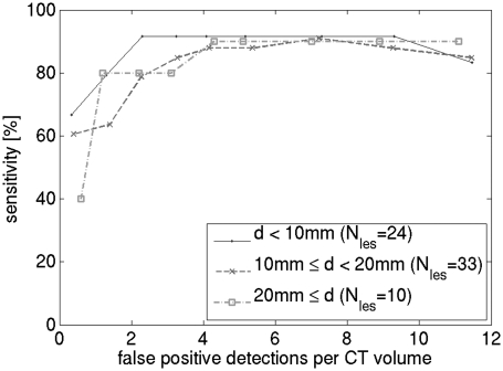
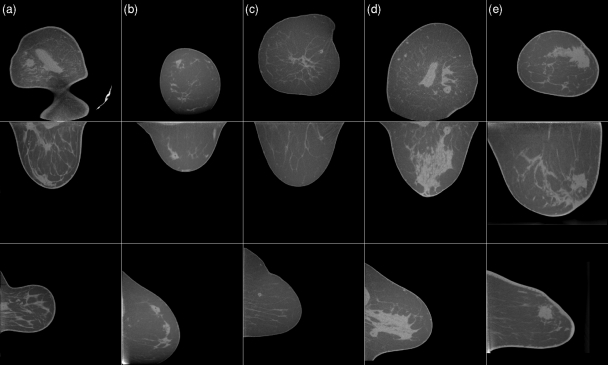
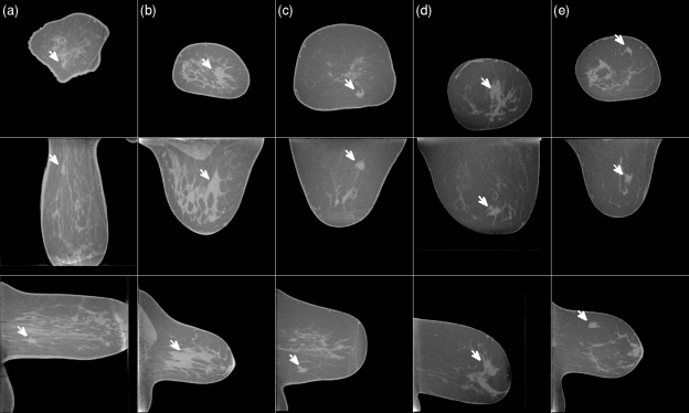
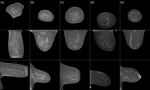
Figure 8 shows the effect of mass size on algorithm performance. BCT cases were divided into three size groups and an FROC curve was plotted for each group. For small masses, a slight increase in sensitivity can be observed. Figure 9 shows examples of true-positive detections of the CADe algorithm. Most of these masses had partially circumscribed margins. Figure 10 shows examples of masses that were missed by the CADe algorithm. Masses that were missed by the algorithm tended to have an irregular shape. Figure 11 shows examples of false positive detections for the cases in which the mass was missed. In a breast in which circumscribed benign lesions were present in addition to a malignant mass, the algorithm tended to be more sensitive to the benign masses [such as for the case shown in Figs. 10c, 11c].

Figure 8.

Effect of lesion size [lesion diameter d] on CADe FROC performance. Cases with multiple lesions, and cases without lesions were excluded from this analysis.

Figure 9.

Examples of true-positive detections. Each column shows the coronal, axial and sagittal slice centered on the mass that is indicated by a red mark. The masses in cases (a),(b),(c),(e) are malignant, and the mass in case (d) is benign. For this display, the axial and sagittal slices were interpolated onto an isotropic 512 × 512 grid. The gray scale window is [−400 HU, 300 HU] and is equal for all slices shown in Figs. 91011. The variation in HU across adipose tissue, and variations in HU across cases, is due to incomplete scatter correction.

Figure 10.

Examples of CT cases in which the lesion was missed by the detection algorithm. As in Fig. 9, each column shows a coronal, axial and sagittal slice centered on the mass. The white arrow indicates the location of the mass. All masses are malignant. The gray scale window is [−400 HU, 300 HU] and is equal for all slices shown in Figs. 91011.

Figure 11.

Examples of false positive detections. The cases shown are the same as those in Fig. 10. The false positive detection is indicated by a red marker. The gray scale window is [−400 HU, 300 HU] and is equal for all slices shown in Figs. 91011.

DISCUSSION

The CADe system for BCT that is described here yielded good performance in this preliminary evaluation. While CADe schemes for mammography have higher performance, typically 83% sensitivity at 1 false detection per image for masses,²⁴ such algorithms are trained on much larger databases and have more than 10 years of development. Perhaps more importantly, a mammogram has a much smaller amount of data compared to BCT. A more fair comparison would be to double the false detection rate for CADe applied to mammography, since there are two views of each breast in mammography compared to a single scan in BCT. The BCT CADe scheme reported here also has comparable performance to the initial CADe schemes for breast tomosynthesis: 80% sensitivity with 1.23 false detections per breast volume as reported by Chan et al.,¹³ and 90% sensitivity with 1.5 false detections per breast volume for our initial scheme.¹⁴

Lesion characteristics of malignant and benign lesions differ, which likely led to a different feature set depending on the mass types used for feature selection. When malignant masses only were considered as actual lesions in feature selection, the step-wise feature selection returned an additional feature. While the difference in feature set did not have a significant effect on performance, at low false positive rates, the feature set based on malignant masses resulted in a slight increase in sensitivity.

The detection performance results indicate that the sensitivity of our CADe scheme is limited by the sensitivity of RGI to nonspherical lesions. RGI is highest when the lesion is spherical with a circumscribed or well-defined margin, and RGI segmentation is effective in determining the margin of a lesion, especially when the boundary is partially obscured. However, while irregularly-shaped lesions are initially well segmented, the subsequent RGI value tends to be low and the lesion may be missed by the CADe scheme, as can be seen in Fig. 8. This may also explain why our CADe scheme performs better on smaller lesions, since smaller lesions tend to be more regular in shape, in part, because the image spatial resolution is too coarse to show the fine detail on a small object. Thus, it may be advantageous to reduce the resolution of VOIs that contain large lesions. In future research, we plan to develop algorithms that can detect irregular and spiculated lesions. On the other hand, contrast-enhanced dedicated breast CT (CEBCT) is currently undergoing clinical research.⁴ CEBCT images might improve CADe performance, since malignant lesions tend to produce strong enhancement.

In traditional CADe algorithms, a prefiltering stage is often used to identify mass candidates at a high sensitivity, followed by a feature extraction and analysis stage.²⁵ In our approach, a full feature set was extracted for the entire glandular region of the breast, which is computationally expensive. However, this eliminates uncertainty in segmentation and feature extraction that results from location uncertainty of mass candidates returned by a prefiltering stage. Another potential benefit of this approach, which we plan to explore in the future, is the potential to increase algorithm sensitivity by merging detection features that are sensitive to different shapes of masses.

The limitation of mass detection in BCT differs from that in mammography and tomosynthesis. In the latter two, lesion detection is limited by breast structure.^{26, 27, 28} On the other hand, in BCT, the breast structure is fully resolved, and lesion detection is limited by contrast. Lesion contrast in BCT is reduced because of the relatively high x-ray tube voltage of 80 kVp, and it is degraded because of the increased scatter, as there is no breast compression or antiscatter grid in BCT. Furthermore, cancerous lesions are stiffer than normal breast tissue,²⁹ thus, breast compression may increase lesion conspicuity on mammography and tomosynthesis.

The main limitation of our study is that the dataset was small. This limits the ability to select the optimum feature set and to train the classifier.^{21, 30} Both of these will decrease the overall performance of our CADe scheme. We believe that a larger database will allow not only for a more accurate CADe scheme to be developed, but will also allow for better testing of the performance and robustness of our CADe scheme.

APPENDIX A: FEATURE SET

The feature set used in this study is described below, where ℜ is the segmented region and M is its margin. ℜ_a is the adipose region in the VOI, ℜ_s is the region covered by an equivalent sphere (where sphere volume and region volume are equal, V_s = V_R). Image gray values are denoted by GV, and the image gradient vector is G with its radial component G_r. Below, <·> denotes average and |.| is the norm of a vector. Units are given where appropriate.

Margin strength descriptors
Average radial gradient	〈Gr(M)〉
Radial gradient index (RGI)	〈Gr(M)〉/〈|G(M)|〉
Relative RGI	RGI/max(RGI)
Margin Strength 1	〈|G(M)|〉/(〈GV(M)〉 − 〈GV(ℜa)〉)
Margin Strength 2	std(|G(M)|)/(〈GV(M)〉 − 〈GV(ℜa)〉)
Radial gradient variation	std(Gr(M))
Shape descriptors
Irregularity	c*ℜ1/3/M1/2 where c is a constant
Compactness	∑ (ℜ ∩ ℜs)/∑ ℜs
Ellipsoid semi-axes minimum to maximum ratio	min(h1,h2,h3)/max(h1,h2,h3) where hi (i = 1,2,3) are the semi-axes of an ellipsoid fit to ℜ
Standard deviation of margin to center distance [mm]	std(|dM|)
Relative standard deviation of margin to center distance	std(|dM|)/〈|dM|〉
average margin alignment: average cosine of polar angle along margin	〈cos(〈(G,r)) (M)〉
Margin volume (mm3)	∑ M
Histogram descriptors
Average region gray value (HU)	〈GV(ℜ)〉
Region contrast (HU)	〈GV(ℜ))〉 − GV(∼ℜ & ℜa)〉
Standard deviation of region gray values (HU)	std(GV(ℜ))〉
Standard deviation of gray values along margin (HU)	std(GV(M))

APPENDIX B: PATIENT SELECTION CRITERIA

All patients over the age of 35, who had BIRADS 4 or 5 lesions were asked to participate in the study by a radiologist at the time they were advised of the need for biopsy of the lesion. Exclusion criteria were: recent breast biopsy, history of allergic reaction to contrast, chronic asthma, allergy to iodine, multiple drug or food allergies, diabetes, serum creatinine over 1.5, renal disease, history of pulmonary disease that would preclude 15 s breath hold. Lesion size was not considered in the recruitment of the subjects.

References

- Berry D. A., Cronin K. A., Plevritis S. K., Fryback D. G., Clarke L., Zelen M., Mandelblatt J. S., Yakovlev A. Y., Habbema J. D. F., and Feuer E. J., “Effect of screening and adjuvant therapy on mortality from breast cancer,” N. Engl. J. Med. 353(17), 1784–1792 (2005). 10.1056/NEJMoa050518 [DOI] [PubMed] [Google Scholar]
- Chen Z. and Ning R., “Why should breast tumour detection go three dimensional?,” Phys. Med. Biol. 48(14), 2217–2228 (2003). 10.1088/0031-9155/48/14/312 [DOI] [PubMed] [Google Scholar]
- O’Connell A., Conover D. L., Zhang Y., Seifert P., Logan-Young W., Lin C. -F. L., Sahler L., and Ning R., “Cone-beam CT for breast imaging: Radiation dose, breast coverage, and image quality,” AJR 195(2), 496–509 (2010). 10.2214/AJR.08.1017 [DOI] [PubMed] [Google Scholar]
- Prionas N. D., Lindfors K. K., Ray S., Huang S.-Y., Beckett L. A., Monsky W. L., and Boone J. M., “Contrast-enhanced dedicated breast CT: Initial clinical experience,” Radiology 256(3), 714–723 (2010). 10.1148/radiol.10092311 [DOI] [PMC free article] [PubMed] [Google Scholar]
- Lindfors K. K., Boone J. M., Nelson T. R., Yang K., Kwan A. L. C., and Miller D. F., “Dedicated breast CT: Initial clinical experience,” Radiology 246(3), 725–733 (2008). 10.1148/radiol.2463070410 [DOI] [PMC free article] [PubMed] [Google Scholar]
- Lindfors K., Boone J., Newell M., and D C.’Orsi, “Dedicated breast computed tomography: The optimal cross-sectional imaging solution?,” Radiol. Clin. North Am. 48(5), 1043–1054 (2010). 10.1016/j.rcl.2010.06.001 [DOI] [PMC free article] [PubMed] [Google Scholar]
- Gromet M., “Comparison of computer-aided detection to double reading of screening mammograms: Review of 231,221 mammograms,” AJR 190(4), 854–859 (2008). 10.2214/AJR.07.2812 [DOI] [PubMed] [Google Scholar]
- Astley S. M. and Gilbert F. J., “Computer-aided detection in mammography,” Clin. Radiol. 59(5), 390–399 (2004). 10.1016/j.crad.2003.11.017 [DOI] [PubMed] [Google Scholar]
- Freer T. W. and Ulissey M. J., “Screening mammography with computer-aided detection: Prospective study of 12,860 patients in a community breast center,” Radiology 220(3), 781 (2001). 10.1148/radiol.2203001282 [DOI] [PubMed] [Google Scholar]
- Birdwell R. L., Bandodkar P., and Ikeda D. M., “Computer-aided detection with screening mammography in a University Hospital Setting,” Radiology 236(2), 451–457 (2005). 10.1148/radiol.2362040864 [DOI] [PubMed] [Google Scholar]
- Morton M., Whaley D., and Brandt K., “Screening mammograms: Interpretation with computer-aided detetion—Prospective evaluation,” Radiology 239(2), 375–383 (2006). 10.1148/radiol.2392042121 [DOI] [PubMed] [Google Scholar]
- Dean J. C. and Ilvento C. C., “Improved cancer detection using computer-aided detection with diagnostic and screening mammography: Prospective study of 104 cancers,” AJR 187(1), 20–28 (2006). 10.2214/AJR.05.0111 [DOI] [PubMed] [Google Scholar]
- Chan H.-P., Wei J., Zhang Y., Helvie M. A., Moore R. H., Sahiner B., Hadjiiski L., and Kopans D. B., “Computer-aided detection of masses in digital tomosynthesis mammography: Comparison of three approaches,” Med. Phys. 35(9), 4087–4095 (2008). 10.1118/1.2968098 [DOI] [PMC free article] [PubMed] [Google Scholar]
- Reiser I., Nishikawa R. M., Giger M. L., Wu T., Rafferty E. A., Moore R., and Kopans D. B., “Computerized mass detection for digital breast tomosynthesis directly from the projection images,” Med. Phys. 33(2), 482 (2006). 10.1118/1.2163390 [DOI] [PubMed] [Google Scholar]
- Singh S., Tourassi G. D., Baker J. A., Samei E., and Lo J. Y., “Automated breast mass detection in 3D reconstructed tomosynthesis volumes: A featureless approach,” Med. Phys. 35(8), 3626–3636 (2008). 10.1118/1.2953562 [DOI] [PMC free article] [PubMed] [Google Scholar]
- American College of Radiology (ACR), Breast Imaging Reporting and Data System Atlas (BI-RADS Atlas) (American College of Radiology, Reston, VA, 2003). [Google Scholar]
- Soille P., Morphological Image Analysis: Principles and Applications (Springer, New York, 1999). [Google Scholar]
- Shih T.-C., Chen J.-H., Liu D., Nie K., Sun L., Lin M., Chang D., Nalcioglu O., and Su M.-Y., “Computational simulation of breast compression based on segmented breast and fibroglandular tissues on magnetic resonance images,” Phys. Med. Biol. 55(14), 4153–4168 (2010). 10.1088/0031-9155/55/14/013 [DOI] [PMC free article] [PubMed] [Google Scholar]
- Kupinski M. and Giger M., “Automated seeded lesion segmentation on digital mammograms,” IEEE Trans. Med. Imaging 17(4), 510–517 (1998). 10.1109/42.730396 [DOI] [PubMed] [Google Scholar]
- Xue J. and Titterington D., “Do unbalanced data have a negative effect on LDA?,” Pattern Recogn. 41(5), 1558–1571 (2008). 10.1016/j.patcog.2007.11.008 [DOI] [Google Scholar]
- Sahiner B., Chan H. P., Petrick N., Wagner R. F., and Hadjiiski L., “Feature selection and classifier performance in computer-aided diagnosis: The effect of finite sample size,” Med. Phys. 27(7), 1509–1522 (2000). 10.1118/1.599017 [DOI] [PMC free article] [PubMed] [Google Scholar]
- Kupinski M. and Giger M. L., “Detection of mass lesions in mammography using feature-filtering techniques,” Med. Phys. 27(6), 1380 (2000). [Google Scholar]
- Yaffe M. J., Boone J. M., Packard N., Alonzo-Proulx O., Huang S.-Y., Peressotti C. L., Al-Mayah A., and Brock K., “The myth of the 50-50 breast,” Med. Phys. 36(12), 5437 (2009). 10.1118/1.3250863 [DOI] [PMC free article] [PubMed] [Google Scholar]
- Petrick N., Sahiner B., Chan H.-P., Helvie M. A., Paquerault S., and Hadjiiski L. M., “Breast cancer detection: Evaluation of a mass-detection algorithm for computer-aided diagnosis experience in 263 patients,” Radiology 224(1), 217–224 (2002). 10.1148/radiol.2241011062 [DOI] [PubMed] [Google Scholar]
- Nishikawa R. M., “Current status and future directions of computer-aided diagnosis in mammography,” Comput. Med. Imaging Graph. 31(4-5), 224–235 (2007). 10.1016/j.compmedimag.2007.02.009 [DOI] [PubMed] [Google Scholar]
- Burgess A. E., Jacobson F. L., and Judy P. F., “Human observer detection experiments with mammograms and power-law noise,” Med. Phys. 28(4), 419 (2001). 10.1118/1.1355308 [DOI] [PubMed] [Google Scholar]
- Metheany K. G., Abbey C. K., Packard N., and Boone J. M., “Characterizing anatomical variability in breast CT images,” Med. Phys. 35(10), 4685 (2008). 10.1118/1.2977772 [DOI] [PMC free article] [PubMed] [Google Scholar]
- Engstrom E., Reiser I., and Nishikawa R., “Comparison of power spectra for tomosynthesis projections and reconstructed images,” Med. Phys. 36(5), 1753 (2009). 10.1118/1.3116774 [DOI] [PMC free article] [PubMed] [Google Scholar]
- Krouskop T. A., Wheeler T. M., Kallel F., Garra B. S., and Hall T., “Elastic moduli of breast and prostate tissues under compression,” Ultrason. Imaging 20(4), 260–274 (1998). [DOI] [PubMed] [Google Scholar]
- Kupinski M. A. and Giger M. L., “Feature selection with limited datasets,” Med. Phys. 26(10), 2176–2182 (1999). 10.1118/1.598821 [DOI] [PubMed] [Google Scholar]