Compressed Sensing Sodium MRI of Cartilage at 7T: Preliminary Study

Abstract

Sodium MRI has been shown to be highly specific for glycosaminoglycan (GAG) content in articular cartilage, the loss of which is an early sign of osteoarthritis (OA). Quantitative sodium MRI techniques are therefore under development in order to detect and assess early biochemical degradation of cartilage, but due to low sodium NMR sensitivity and its low concentration, sodium images need long acquisition times (15 to 25 min) even at high magnetic fields and are typically of low resolution. In this preliminary study, we show that compressed sensing can be applied to reduce the acquisition time by a factor of 2 at 7T without losing sodium quantification accuracy. Alternatively, the nonlinear reconstruction technique can be used to denoise fully-sampled images. We expect to even further reduce this acquisition time by using parallel imaging techniques combined with SNR-improved 3D sequences at 3T and 7T.

Introduction

Osteoarthritis (OA) is the most common form of arthritis in synovial joints and a leading cause of chronic disability, mainly in the elderly population. In 2008, it was estimated that nearly 27 million adults in the United States (9% of the population) have clinical OA. It is predicted that by the year 2030, nearly 67 million adults (19% of the US population) will be affected by OA [1, 2]. There is no known cure for OA and present treatments focus mainly on pain management and ultimately, joint replacement. There are many obstacles to studying OA, including heterogeneity in etiology, variability in progression of disease, and long time periods required to see morphological and structural joint changes. Consequently, we currently lack the ability to predict the course of the disease in individual patients. Therefore, there is a high demand for the development of reliable, objective, non-invasive, and rapid quantitative imaging biomarkers. From a biochemical point of view, OA is a degenerative disease of articular cartilage and is mainly characterized by a loss of glycosaminoglycans (GAGs), a possible change in size and organization of collagen fibers, and by increased water content. Functional magnetic resonance imaging (MRI) techniques are under development to detect biochemical changes in cartilage such as T_1ρ mapping [3], T₂ mapping [4], delayed Gadolinium-enhanced MRI of cartilage (dGEMRIC) [5], GAG chemical exchange saturation transfer (gagCEST) [6], diffusion MRI [7] and sodium (²³Na) MRI [8–10]. All these methods have their own advantages and disadvantages [11, 12], but quantitative sodium MRI has been shown to be highly specific for the GAG content in cartilage [9, 13, 14]. Quantitative sodium MRI could therefore be used as a means of detection and assessment of the degree of biochemical degradation of cartilage in very early stages of OA [8–10, 13–16]. Recent technological developments such as high magnetic field scanners, novel ultrashort echo time (UTE) pulse sequences, multi-channel radiofrequency (RF) arrays and non-Cartesian reconstruction methods have great potential for improving the performance of multinuclear imaging. However, due to the low sodium concentration in vivo and its low NMR sensitivity, imaging of sodium in cartilage still requires long acquisition times (15–20 min for usual sodium 3D images and 25 min for fluid suppressed images) with relatively low resolution [17–19].

Compressed sensing (CS) is a powerful method for image reconstruction which enables reduced imaging time by k-space undersampling. It has been under development since 2006 [20] and has been successfully applied to proton and ³He MRI [21–23], ¹³C and ¹⁹F spectroscopy [24, 25], and to microfluidic flow imaging [26], as well as to combined time/k-space domain imaging [27–29]. CS is based on the sparsity (or compressibility) of the image in any known transform domain, the incoherence of the undersampling artifacts, and a dedicated nonlinear reconstruction algorithm. Sodium MRI of articular cartilage is intrinsically sparse and is therefore a good candidate for CS that should allow reconstruction of images from undersampled data within clinically feasible acquisition times (on the order of 10 min or less).

In this work, compressed sensing is applied to undersample a 3D radial pulse sequence for sodium MRI at high field (7T). The nonlinear reconstruction used in CS is also proposed to denoise fully-sampled images.

Materials and Methods

Acquisition Protocol

Data acquisition was performed in vivo on 4 asymptomatic volunteers (2 males, 2 females, average age: 36±15 years) with a 3D radial sequence on a 7T whole-body scanner (Siemens Medical Solution, Erlangen, Germany), with a transmit/receive sodium RF knee coil (quadrature, birdcage) single-tuned at 78.6 MHz (Rapid MR International, Columbus), length 27 cm, and inner diameter 21 cm. Acquisition parameters for a fully sampled data set were: 10,000 projections, TE = 0.15 ms, TR = 100 ms, RF pulse flip angle = 90° of duration 500 μs, time of acquisition = 17 min. Note that the TE was calculated from the end of the RF pulse to the beginning of the data acquisition. The study was approved by the institutional review board and the volunteers signed an informed consent form prior to the experiment. The field-of-view (FOV) was chosen as 200 mm isotropic in order to keep a constant FOV for all volunteers who may have different knee sizes, and so that the calibration phantoms used for sodium quantification all lie within the FOV (see the Tissue Sodium Concentration (TSC) Quantification section).

Standard Image Reconstruction

Once the fully sampled data was acquired, images were reconstructed off-line in Matlab (Mathworks, Natick, MA, USA) with a non-uniform Fast Fourier Transform (NUFFT) regridding algorithm as described in [17, 30, 31]. All images were reconstructed as isotropic 100×100×100 voxels images, resulting in a nominal isotropic resolution of 2 mm. The R factors (acceleration rates) denote the degree of undersampling as follows:

• R=1: Fully sampled data.

• R=2, 3, 4: 50%, 33% and 25% of the radial projections were randomly chosen and kept from the original data; the other projections were assigned a value of 0. This random sampling was applied 100 times for each R factor (2, 3, and 4).

Compressed Sensing (CS)

CS aims to accurately reconstruct certain signals and images from undersampled data acquired below the Nyquist rate. Three requirements are necessary to apply CS [20–22, 32]:

1. Sparsity: The desired image must have a sparse representation in a known transform domain (it must be compressible): it must be composed of a few high-value coefficients and many low-value coefficients, so that thresholding the low-value coefficients does not degrade the image quality too much. Usual sparsifying transforms are the discrete wavelet transform (DWT), discrete cosine transform (DCT), and finite differences. Sodium cartilage images acquired in this study are intrinsically sparse in the image domain as the strongest signals of interest occur only in ~20% of the voxels in the 3D image.

2. Incoherence: The measurement basis and the sparse representation basis must be uncorrelated, so that the k-space undersampling artifacts add incoherently to the sparse signal coefficients. Thus, non-Cartesian data sampling is preferred for the design of sampling trajectories with low coherence. The 3D radial acquisition already fulfills this requirement as the spherical coordinates of the spokes in our acquisition scheme are chosen following the Rakhmanov-Saff-Zhou algorithm [33,34] in order to achieve a homogeneous distribution of the data along the radial views in a sphere. Most of the acquired data points are therefore away from the Cartesian grid.

3. Nonlinear reconstruction: The image should be reconstructed by a nonlinear method that enforces both sparsity of the image representation in the transform domain and consistency of the reconstruction with the acquired samples. The image x is reconstructed from the acquired data y by minimizing the function f(x):

   $$\text{f}(\text{x})={\left|\right|\mathcal{F}\text{x}-\text{y}\left|\right|}_2^2+{\lambda }_1{\left|\right|\psi \text{x}\left|\right|}_1+{\lambda }_2\text{TV}(\text{x}),$$ (1)

   where ||x||₁ = Σ_i|x_i| represents the ℓ₁ norm, ${\left|\right|\text{x}\left|\right|}_2=\sqrt{{\sum }_{\text{i}}{\mid {\text{x}}_{\text{i}}\mid }^2}$ is the ℓ₂ norm, denotes the (Cartesian) FFT, ψ is the sparsifying transform and TV(x) represents the total variation of the image x (sum of the absolute variations of the image). Minimizing the ℓ₁ norm promotes the sparsity while minimizing the ℓ₂ norm enforces the data consistency. TV is a finite difference transform and it is often useful to add it as a penalty in order to increase the sparsity of the image in both the transform domain ψ and in the finite difference domain. λ₁ and λ₂ are weighting factors for the ℓ₁ and ℓ₂ norms respectively. Minimization of f(x) was performed in Matlab (Mathworks, natick, MA, USA) using the nonlinear conjugate gradient method.

In this study, CS was applied on the normalized 3D regridded Cartesian k-space y of the images (after NUFFT reconstruction with R=1, 2, 3 and 4), which was used for data consistency. The CS algorithm for reconstructing x was applied with 72 iterations and tested over a range of values for λ₁ and λ₂: λ₁ =0.0005, 0.0010, 0.0025, 0.0050, 0.0075, 0.0100 and λ₂ =0, 0.0005, 0.0010, 0.0025, 0.0050, 0.0075, 0.0100. The CS algorithm was tested with ψ=1 (no sparsifying transform) on all volunteers and also with ψ= DCT on one volunteer. The average reconstruction time for each pair λ₁/λ₂ was 5–10 min when ψ =1 and 9–20 min when ψ= DCT.

SNR Measurements

Signal-to-noise ratio (SNR) measurement is a difficult task on images obtained from nonlinear reconstructions methods such as NUFFT and CS. In order to be able to fairly compare the SNR of images reconstructed with and without CS after NUFFT, 100 random samplings of the data were used to obtain more uniform distribution of the noise for all the images. The statistical standard deviation (STD) of all the voxels over these 100 randomly sampled reconstructed images was calculated for R=2, 3 and 4, with and without CS applied after the NUFFT reconstruction. The distribution of the std of noise (from 20 slices outside the knee anatomy) was very similar to a normal distribution (see Figure 1, red fit) in all cases. This is to be expected for a large number of values (N=100) for which the STD is calculated (the χ² distribution of STD becomes a normal distribution when N>50 [35]). Note that since for R=1 the full data cannot be randomly resampled, STD was extrapolated with a linear fit as a function of $\sqrt{\text{R}}$ (See Figure 2). The mean image (over 100 random samplings) was also calculated for R=2, 3, and 4. The mean signal in cartilage was then measured in selected ROIs of 30 voxels in 4 different regions in the cartilage over 4 consecutive slices of these mean images. The cartilage regions were: patellar (abbreviation: PAT), femorotibial medial (MED), femorotibial lateral (LAT), and posterior femoral condyle (CON). The SNR of the images for each R was then calculated as: SNR = mean cartilage signal divided by mean STD of noise.

Figure 1.

Example of distribution of the standard deviations (STD) of the noise for R=2, 3 and 4, for NUFFT (green) and NUFFT+CS (blue) and their best fit with a normal distribution (red curve), from one volunteer. Histograms were calculated from the STD of all the voxels of the 10 first and 10 last coronal slices of the 3D data (200,000 voxels) from one volunteer. STD of noise was calculated from 100 reconstructions with random sampling of the 10,000 acquired radial views for R=2, 3 and 4.

Figure 2.

Linear fit of mean STD of noise from data with R=2,3 and 4, for all 4 volunteers (Vol.), and 2 reconstruction methods (NUFFT and NUFFT+CS). Red dots: Extrapolated mean STD of the noise for R=1 estimated from the linear fit of the data measured with R=2,3 and 4, as a function of $\sqrt{\text{R}}$. 1: Vol. 3, NUFFT. 2: Vol. 4, NUFFT. 3: Vol. 3, NUFFT+CS. 4: Vol. 2, NUFFT. 5: Vol. 1, NUFFT. 6: Vol. 4, NUFFT+CS. 7: Vol. 2, NUFFT+CS. 8: Vol. 1, NUFFT+CS.

Tissue Sodium Concentration (TSC) Quantification

The images were acquired with calibration tube phantoms that were placed on the knee cap and included in the FOV. Sodium quantitation was then performed using linear regression in Matlab as follows: ROIs were drawn in 4 calibration phantoms (150, 200, 250 and 300 mM NaCl) and their average signal intensities were corrected for T1, $\text{T}{2}_{\text{short}}^{\ast }$ and $\text{T}{2}_{\text{long}}^{\ast }$ of the gels as described in [17]. Another ROI was drawn in the noise area and the mean value of the noise was used as a 0 mM sodium concentration phantom. A linear regression curve of these corrected phantom intensities and noise versus sodium concentrations was then calculated and used to extrapolate the sodium 3D maps of the whole sample. After the regression curve calculation from the gel signals but before extrapolation of the images to sodium maps, the images were also corrected for the T1, $\text{T}{2}_{\text{short}}^{\ast }$ and $\text{T}{2}_{\text{long}}^{\ast }$ of cartilage measured in vivo [36]. As 75% of the volume in cartilage is extracellular and composed of water, and sodium ions are mainly present in this space, the sodium maps were divided by 0.75 in order to obtain the real sodium concentration [37, 38]. Less than 5% of the cartilage volume is composed of cells [39] and the intracellular sodium concentration, estimated around 5–10 mM, can therefore be considered negligible in the present study.

Mean sodium concentrations in the 4 different regions of the cartilage were measured with exactly the same protocol used for measuring the signal (same slices, same ROIs) as described in the SNR measurements section.

Statistical Analysis

For each volunteer and each region in cartilage, a Student’s t-test was applied to the resulting sets of pixels (120 voxels) from the ROIs (30 voxels × 4 slices) on the TSC maps in order to compare all the CS data with the original fully sampled data (NUFFT, R=1, without CS). Statistical significance was defined as the condition that p<0.05.

Results and Discussion

Examples of sodium images and TSC maps from one volunteer are shown in Figures 3 and 4 on a coronal plane, for CS parameters λ₁=0.0005, λ₂=0.0005. Mean SNR and TSC measurements and p values over all volunteers are given in Tables 1 and 2. SNR was increased when CS was applied directly on fully sampled data for denoising (+69% on average), and slightly decreased for R=2 data (−20% on average) compared to fully sampled data (R=1). TSC of the cartilage looked very similar (within the standard deviation) within the 4 regions of cartilage for all R values, with and without CS applied, but these values are not a sufficient parameters to validate the accuracy of the measurements. CS data were considered as valid data for sodium quantification when both of the following conditions were fulfilled for all volunteers:

Figure 3.

Example of sodium images obtained from one volunteer with NUFFT without CS and with CS, with the parameters λ₁=0.0005, λ₂=0.0005 and ψ=1, for acceleration factors R=1, 2, 3 and 4.

Figure 4.

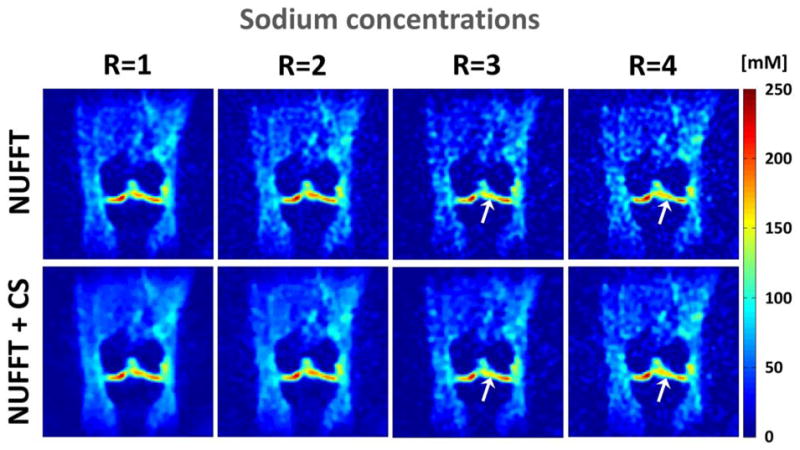
Tissue Sodium Concentrations (TSC) in mM corresponding to the images shown in Fig. 3 obtained with NUFFT without CS and with CS, with the parameters λ₁=0.0005, λ₂=0.0005, for acceleration factors R=1, 2, 3 and 4. The white arrows indicate zones in the femorotibial lateral cartilage where a loss of sodium concentration seems to appear in the data with R=3 and 4 (with and without CS), and which could be misinterpreted as a loss of GAG in cartilage.

Table 1.

Mean SNR in 4 regions of the cartilage for CS parameters: λ₁=0.0005, λ₂=0.0005 and ψ=1. Each mean±standard deviation of SNR corresponds to the mean value over all volunteers of the SNR measured over 4 consecutive slices for each region and each volunteer. The values in the % columns correspond to the variation of SNR in % of the reference value for each column (NUFFT with R=1, gray row). The numbers in bold correspond to the increased or equal SNR values compared to the reference SNR. Abbreviations: PAT=Patellar, MED=FT Medial, LAT= FT Lateral, CON=PF Condyle, with PF=Posterior Femoral, FT=Femoro-Tibial.

SNR		PAT		MED		LAT		CON
Recon.	R	SNR	%	SNR	%	SNR	%	SNR	%
NUFFT	1	43.8±7.5	0	43.8±6.2	0	42.5±3.4	0	45.3±6.4	0
	2	26.4±4.5	−40	26.3±3.4	−40	25.6±2.1	−40	27.3±3.9	−40
	3	19.9±3.3	−55	19.8±2.6	−55	19.2±1.6	−55	20.5±2.9	−55
	4	16.8±2.9	−62	16.9±2.6	−61	16.3±1.3	−62	17.5±2.5	−61
NUFFT + CS	1	73.9±13.1	+69	74.4±12.4	+70	71.7±6.4	+69	76.7±13.0	+69
	2	35.0±6.2	−20	35.2±5.0	−20	34.0±2.9	−20	36.3±5.8	−20
	3	24.5±4.2	−44	24.6±3.5	−44	23.8±2.0	−44	25.4±3.9	−44
	4	20.0±3.5	−54	20.2±2.7	−54	19.4±1.6	−54	20.9±3.2	−54

Table 2.

Tissue Sodium Concentrations (TSC) in mM.

Mean Tissue Sodium Concentration (TSC) in mM in 4 regions of the cartilage for CS parameters: λ₁=0.0005, λ₂=0.0005 and ψ=1. Each mean±standard deviation of TSC corresponds to the mean value over all volunteers of the TSC measured over 4 consecutive slices for each region and each volunteer. The same regions of interests (ROIs) were used to compare measurements with different acceleration rates R for reconstruction. The reference TSC (NUFFT with R=1) are shown in the gray row. Mean P values over all volunteers were measured with a Student’s t-test for comparing TSC measured in all voxels of the 4 ROIs (on 4 consecutive slices) to the reference data. Abbreviations: PAT=Patellar, MED=FT Medial, LAT= FT Lateral, CON=PF Condyle, with PF=Posterior Femoral, FT=Femoro-Tibial.

Recon.	R	PAT	p	MED	p	LAT	p	CON	p
NUFFT	1	171±42	1	172±24	1	165±3	1	160±9	1
	2	171±44	0.513±0.161	174±24	0.663±0.204	165±29	0.695±0.301	161±9	0.724±0.255
	3	170±40	0.037±0.033	171±22	0.545±0.303	163±27	0.472±0.342	158±7	0.571±0.328
	4	171±45	0.243±0.192	173±22	0.510±0.265	165±31	0.392±0.369	162±8	0.376±0.297
NUFFT + CS	1	170±42	0.600±0.170	172±24	0.882±0.076	164±27	0.624±0.284	159±9	0.833±0.149
	2	171±43	0.531±0.236	173±24	0.654±0.179	164±28	0.624±0.247	160±9	0.666±0.171
	3	165±39	0.014±0.011	171±23	0.592±0.221	163±27	0.335±0.295	158±7	0.549±0.368
	4	170±45	0.371±0.374	173±23	0.506±0.212	164±30	0.395±0.249	161±8	0.403±0.228

1. All data were compared visually with the original fully sampled image (NUFFT, R=1, without CS) in order to detect artifacts and local modifications of the signal that could be misinterpreted as a loss of sodium (such regions are indicated by arrows in Figure 4 for R=3 and 4). Most of the data with large TV weighting (λ₂>0.0010) were too blurred to give accurate estimation of the TSC and details in cartilage, and were therefore rejected.

2. . Only CS data where the t-test showed a non-significant difference in all of the 4 regions of the cartilage compared to the fully sampled data were considered as valid. From this selection method, the only valid pairs of CS parameters λ₁/λ₂ were 0.0005/0, 0.0005/0.0005, 0.0010/0, for all volunteers (but also 0.0010/0.0005 and 0.0025/0 for 3 of them), for ψ=1, for R=1, 2 and 4 only. When ψ=DCT, the only valid pairs of CS parameters λ₁/λ₂ were 0.0005/0 and 0.0005/0.0005, for R=1, 2 and 4 only. CS data obtained from R=3 always show a significant difference (p<0.05) to fully sampled data in at least one part of the cartilage, for all the volunteers (see Table 2).

Although R=4 (with and without CS) can give some results similar to fully sampled data for the average TSC (p>0.05), some parts of cartilage show a loss of sodium signal mainly due to reconstruction and undersampling that could be misinterpreted as a real loss of GAG, as shown on Figure 4 (white arrows). R=3 and 4 seem therefore to be too high undersampling rates and may lead to statistically significant differences in TSC measurements compared to fully sampled data and also to possible misinterpretation of the images. CS can therefore be used to either de-noise fully sampled data (R=1) in order to increase the SNR and therefore potentially increase the accuracy in sodium quantification, or on undersampled data with R=2 to decrease the total acquisition time without losing TSC accuracy. The application of a sparsifying transform such as DCT is not necessary for the present purpose, which is cartilage sodium imaging in the knee, as it generates similar results than ψ=1. The sodium cartilage images are sparse enough for applying CS on the image domain itself, and CS reconstruction is therefore faster (~5 min with ψ=1 instead of ~9 min with ψ=DCT).

For verification, the CS method was also applied on data acquired with undersampling rates R=1 (8000 projections), R=2 (4000 projections) and R=4 (2000 projections) on another volunteer, and the resulting images were compared to the images obtained from the CS method applied to simulated R factors on fully sampled data as described in the Materials and Methods\Standard Image Reconstruction section. Both methods showed identical results.

Conclusion

This preliminary study shows that CS can be applied to sodium MRI of cartilage at 7T in order to decrease the acquisition time by a factor of 2 without losing accuracy in TSC over different regions of interest in the cartilage for detecting early signs of OA. Further studies will involve testing the application of the CS technique to data acquired at 3T, with and without fluid suppression at both 3T and 7T, combined with new 3D radial based sequences such as density adapted 3D radial [40], Twisted projection imaging (TPI) [41] or 3D cones [42] which allow increases in SNR. Further improvements could be obtained by combining CS with NUFFT in the iterative process (as in Equation 1), instead of simply working with the Cartesian k-space (obtained after one NUFFT reconstruction) for the data consistency part of Equation 1. This step, however, is by no means obvious, as the NUFFT algorithm applied from Cartesian to radial data can induce errors that can propagate during the CS algorithm, and as a result reduce the efficiency of the technique.

A further improvement, upon acquisition of multichannel double-tuned (¹H+²³Na) RF knee coils at 3T and 7T, would be to apply CS Sodium MRI in combination with parallel imaging to further reduce the imaging time by another factor 2 or 3. Such approaches are already under development in our center for dynamic proton MRI [43, 44].

Highlights.

• Sodium MRI may assess early osteoarthritis but requires long acquisition times.

• Compressed sensing can reduce the acquisition time by 2 at 7T without accuracy loss.

• This nonlinear reconstruction technique can also denoise fully-sampled images.

References

- 1.Lawrence R, Felson D, Helmick C, Arnold L, Choi H, Deyo R, Gabriel S, Hirsch R, Hochberg M, Hunder G, et al. Estimates of the prevalence of arthritis and other rheumatic conditions in the United States: Part II. Arthritis & Rheumatism. 2008;58(1):26–35. doi: 10.1002/art.23176. [DOI] [PMC free article] [PubMed] [Google Scholar]
- 2.Kotlarz H, Gunnarsson C, Fang H, Rizzo J. Insurer and out-of-pocket costs of osteoarthritis in the US: Evidence from national survey data. Arthritis & Rheumatism. 2009;60(12):3546–3553. doi: 10.1002/art.24984. [DOI] [PubMed] [Google Scholar]
- 3.Regatte R, Akella S, Borthakur A, Kneeland J, Reddy R. In Vivo Proton MR Three-dimensional T1ρ Mapping of Human Articular Cartilage: Initial Experience. Radiology. 2003;229(1):269. doi: 10.1148/radiol.2291021041. [DOI] [PubMed] [Google Scholar]
- 4.Mosher T, Dardzinski B. Cartilage MRI T2 relaxation time mapping: overview and applications. Seminars in musculoskeletal radiology. 2004;8:355–368. doi: 10.1055/s-2004-861764. [DOI] [PubMed] [Google Scholar]
- 5.Bashir A, Gray M, Burstein D. Gd-DTPA2-as a measure of cartilage degradation. Magnetic Resonance in Medicine. 1996;36(5):665–673. doi: 10.1002/mrm.1910360504. [DOI] [PubMed] [Google Scholar]
- 6.Ling W, Regatte R, Navon G, Jerschow A. Assessment of glycosaminoglycan concentration in vivo by chemical exchange-dependent saturation transfer (gagCEST) Proceedings of the National Academy of Sciences. 2008;105(7):2266. doi: 10.1073/pnas.0707666105. [DOI] [PMC free article] [PubMed] [Google Scholar]
- 7.Filidoro L, Dietrich O, Weber J, Rauch E, Oerther T, Wick M, Reiser M, Glaser C. High-resolution diffusion tensor imaging of human patellar cartilage: Feasibility and preliminary findings. Magnetic Resonance in Medicine. 2005;53(5):993–998. doi: 10.1002/mrm.20469. [DOI] [PubMed] [Google Scholar]
- 8.Reddy R, Insko E, Noyszewski E, Dandora R, Kneeland J, Leigh J. Sodium MRI of human articular cartilage in vivo. Magnetic Resonance in Medicine. 1998;39(5):697–701. doi: 10.1002/mrm.1910390505. [DOI] [PubMed] [Google Scholar]
- 9.Shapiro E, Borthakur A, Gougoutas A, Reddy R. 23Na MRI accurately measures fixed charge density in articular cartilage. Magnetic Resonance in Medicine. 2002;47(2):284–291. doi: 10.1002/mrm.10054. [DOI] [PMC free article] [PubMed] [Google Scholar]
- 10.Wang L, Wu Y, Chang G, Oesingmann N, Schweitzer M, Jerschow A, Regatte R. Rapid isotropic 3D-sodium MRI of the knee joint in vivo at 7T. Journal of Magnetic Resonance Imaging. 2009;30(3):606–614. doi: 10.1002/jmri.21881. [DOI] [PMC free article] [PubMed] [Google Scholar]
- 11.Regatte R, Schweitzer M. Novel contrast mechanisms at 3 Tesla and 7 Tesla. Semin Musculoskelet Radiol. 2008;12(3):266–280. doi: 10.1055/s-0028-1083109. [DOI] [PMC free article] [PubMed] [Google Scholar]
- 12.Gold G, Chen C, Koo S, Hargreaves B, Bangerter N. Recent advances in MRI of articular cartilage. American Journal of Roentgenology. 2009;193(3):628. doi: 10.2214/AJR.09.3042. [DOI] [PMC free article] [PubMed] [Google Scholar]
- 13.Lesperance L, Gray M, Burstein D. Determination of fixed charge density in cartilage using nuclear magnetic resonance. Journal of Orthopaedic Research. 1992;10(1):1–13. doi: 10.1002/jor.1100100102. [DOI] [PubMed] [Google Scholar]
- 14.Borthakur A, Mellon E, Niyogi S, Witschey W, Kneeland J, Reddy R. Sodium and T1ρ MRI for molecular and diagnostic imaging of articular cartilage. NMR in Biomedicine. 2006;19(7):781–821. doi: 10.1002/nbm.1102. [DOI] [PMC free article] [PubMed] [Google Scholar]
- 15.Borthakur A, Shapiro E, Beers J, Kudchodkar S, Kneeland J, Reddy R. Sensitivity of MRI to proteoglycan depletion in cartilage: comparison of sodium and proton MRI. Osteoarthritis and Cartilage. 2000;8(4):288–293. doi: 10.1053/joca.1999.0303. [DOI] [PubMed] [Google Scholar]
- 16.Shapiro E, Borthakur A, Dandora R, Kriss A, Leigh J, Reddy R. Sodium visibility and quantitation in intact bovine articular cartilage using high field 23Na MRI and MRS. Journal of Magnetic Resonance. 2000;142(1):24–31. doi: 10.1006/jmre.1999.1932. [DOI] [PubMed] [Google Scholar]
- 17.Madelin G, Lee J, Inati S, Jerschow A, Regatte R. Sodium Inversion Recovery MRI of the Knee Joint In Vivo at 7T. Journal of Magnetic Resonance. 2010;207:42–52. doi: 10.1016/j.jmr.2010.08.003. [DOI] [PMC free article] [PubMed] [Google Scholar]
- 18.Madelin G, Jerschow A, Regatte R. Sodium MRI with fluid suppression: will it improve early detection of osteoarthritis? Imaging in Medicine. 2011;3(1):1–4. [Google Scholar]
- 19.Higgs R. Osteoarthritis: Concentrated efforts to detect early OA. Nature Reviews Rheumatology. 2010;6(11):616. doi: 10.1038/nrrheum.2010.165. [DOI] [PubMed] [Google Scholar]
- 20.Candès E, Romberg J, Tao T. Robust uncertainty principles: Exact signal reconstruction from highly incomplete frequency information, Information Theory. IEEE Transactions on. 2006;52(2):489–509. [Google Scholar]
- 21.Lustig M, Donoho D, Pauly J. Sparse MRI: The application of compressed sensing for rapid MR imaging. Magnetic Resonance in Medicine. 2007;58(6):1182–1195. doi: 10.1002/mrm.21391. [DOI] [PubMed] [Google Scholar]
- 22.Lustig M, Donoho D, Santos J, Pauly J. Compressed sensing MRI, Signal Processing Magazine. IEEE. 2008;25(2):72–82. [Google Scholar]
- 23.Ajraoui S, Lee K, Deppe M, Parnell S, Parra-Robles J, Wild J. Compressed sensing in hyperpolarized 3He Lung MRI. Magnetic Resonance in Medicine. 2010;63(4):1059–1069. doi: 10.1002/mrm.22302. [DOI] [PubMed] [Google Scholar]
- 24.Hu S, Lustig M, Balakrishnan A, Larson P, Bok R, Kurhanewicz J, Nelson S, Goga A, Pauly J, Vigneron D. 3D compressed sensing for highly accelerated hyperpolarized 13C MRSI with in vivo applications to transgenic mouse models of cancer. Magnetic Resonance in Medicine. 2010;63(2):312–321. doi: 10.1002/mrm.22233. [DOI] [PMC free article] [PubMed] [Google Scholar]
- 25.Kampf T, Fischer A, Basse-Lüsebrink T, Ladewig G, Breuer F, Stoll G, Jakob P, Bauer W. Application of Compressed Sensing to in vivo 3D 19F CSI. Journal of Magnetic Resonance. 2010;207:262–273. doi: 10.1016/j.jmr.2010.09.006. [DOI] [PubMed] [Google Scholar]
- 26.Paulsen J, Bajaj V, Pines A. Compressed sensing of remotely detected mri velocimetry in microfluidics. Journal of Magnetic Resonance. 2010;205(2):196–201. doi: 10.1016/j.jmr.2010.04.016. [DOI] [PubMed] [Google Scholar]
- 27.Lustig M, Santos J, Donoho D, Pauly J. kt sparse: High frame rate dynamic mri exploiting spatio-temporal sparsity. Proceedings of the 13th Annual Meeting of ISMRM; Seattle. 2006. p. 2420. [Google Scholar]
- 28.Gamper U, Boesiger P, Kozerke S. Compressed sensing in dynamic mri. Magnetic Resonance in Medicine. 2008;59(2):365–373. doi: 10.1002/mrm.21477. [DOI] [PubMed] [Google Scholar]
- 29.Jung H, Sung K, Nayak K, Kim E, Ye J. k-t focuss: A general compressed sensing framework for high resolution dynamic mri. Magnetic Resonance in Medicine. 2009;61(1):103–116. doi: 10.1002/mrm.21757. [DOI] [PubMed] [Google Scholar]
- 30.Greengard L, Lee J. Accelerating the nonuniform fast Fourier transform. SIAM review. 2004;46(3):443–454. [Google Scholar]
- 31.Greengard L, Lee J, Inati S. The fast sinc transform and image reconstruction from nonuniform samples in k-space. Commun Appl Math and Comput Sci. 2006;1(1):121–131. [Google Scholar]
- 32.Candès E, Wakin M. An introduction to compressive sampling, Signal Processing Magazine. IEEE. 2008;25(2):21–30. [Google Scholar]
- 33.Saff E, Kuijlaars A. Distributing many points on a sphere. The Mathematical Intelligencer. 1997;19(1):5–11. [Google Scholar]
- 34.Rakhmanov E, Saff E, Zhou Y. Minimal discrete energy on the sphere. Math Res Lett. 1994;1(6):647–662. [Google Scholar]
- 35.Box G, Hunter J, Hunter W. Statistics for experimenters: design, innovation, and discovery. 2. 2005. [Google Scholar]
- 36.Madelin G, Jerschow A, Regatte R. Sodium relaxation times in the knee joint in vivo at 7t. NMR in Biomedicine. 2011;XX(XX):XX–XX. doi: 10.1002/nbm.1768. in print. [DOI] [PMC free article] [PubMed] [Google Scholar]
- 37.Shapiro E, Borthakur A, Kaufman J, Leigh J, Reddy R. Water distribution patterns inside bovine articular cartilage as visualized by1H magnetic resonance imaging. Osteoarthritis and Cartilage. 2001;9(6):533–538. doi: 10.1053/joca.2001.0428. [DOI] [PubMed] [Google Scholar]
- 38.Borthakur A, Shapiro E, Akella S, Gougoutas A, Kneeland J, Reddy R. Quantifying Sodium in the Human Wrist in Vivo by Using MR Imaging1. Radiology. 2002;224(2):598. doi: 10.1148/radiol.2242011039. [DOI] [PubMed] [Google Scholar]
- 39.Kuettner K. Biochemistry of articular cartilage in health and disease. Clinical Biochemistry. 1992;25(3):155–163. doi: 10.1016/0009-9120(92)90224-g. [DOI] [PubMed] [Google Scholar]
- 40.Nagel A, Laun F, Weber M, Matthies C, Semmler W, Schad L. Sodium MRI using a density-adapted 3D radial acquisition technique. Magnetic Resonance in Medicine. 2009;62(6):1565–1573. doi: 10.1002/mrm.22157. [DOI] [PubMed] [Google Scholar]
- 41.Boada F, Gillen J, Shen G, Chang S, Thulborn K. Fast three dimensional sodium imaging. Magnetic Resonance in Medicine. 1997;37(5):706–715. doi: 10.1002/mrm.1910370512. [DOI] [PubMed] [Google Scholar]
- 42.Gurney P, Hargreaves B, Nishimura D. Design and analysis of a practical 3D cones trajectory. Magnetic resonance in medicine. 2006;55(3):575–582. doi: 10.1002/mrm.20796. [DOI] [PubMed] [Google Scholar]
- 43.Otazo R, Sodickson D. Distributed compressed sensing for accelerated MRI. Proc Intl Soc Mag Reson Med. 2009;17:377. [Google Scholar]
- 44.Otazo R, Kim D, Axel L, Sodickson D. Combination of compressed sensing and parallel imaging for highly accelerated first-pass cardiac perfusion MRI. Magnetic Resonance in Medicine. 2010;64(3):767–776. doi: 10.1002/mrm.22463. [DOI] [PMC free article] [PubMed] [Google Scholar]