An Algorithm for 353 Odor Detection Thresholds in Humans

Abstract

One hundred and ninety three odor detection thresholds, ODTs, obtained by Nagata using the Japanese triangular bag method can be correlated as log (1/ODT) by a linear equation with R² = 0.748 and a standard deviation, SD, of 0.830 log units; the latter may be compared with our estimate of 0.66 log units for the self-consistency of Nagata's data. Aldehydes, acids, unsaturated esters, and mercaptans were included in the equation through indicator variables that took into account the higher potency of these compounds. The ODTs obtained by Cometto-Muñiz and Cain, by Cometto-Muñiz and Abraham, and by Hellman and Small could be put on the same scale as those of Nagata to yield a linear equation for 353 ODTs with R² = 0.759 and SD = 0.819 log units. The compound descriptors are available for several thousand compounds, and can be calculated from structure, so that further ODT values on the Nagata scale can be predicted for a host of volatile or semivolatile compounds.

Introduction

An odor detection threshold (ODT) is a biological endpoint that provides a quantitative assessment of the effect of airborne chemicals on the olfactory system of a human subject. ODTs, obtained by approximately the same protocol, for a series of chemicals then constitute a suitable measure of the relative effectiveness, or potency, of the chemicals to elicit an effect. The smaller the ODT, the more “potent” is the chemical. Unfortunately, if ODTs are determined by 2 different protocols, the obtained ODT for a particular compound may differ by orders of magnitude, as illustrated for a series of n-alcohols (Cometto-Muñiz and Abraham 2008a). However, their analysis showed that although there were striking differences in the obtained ODT values as between different protocols, there was a clear trend of decreasing ODT values with increasing carbon number of the n-alcohol, that is, along the homologous series. It has been pointed out (Schmidt and Cain 2006) that in cases where different protocols give rise to very different obtained values of ODT, the protocol that gives rise to the lowest obtained values will usually be regarded as the most meaningful. It is generally acknowledged that weaknesses in methodology, for example, poor control of concentration, will result in higher rather than in lower thresholds.

Among other studies cited in comprehensive compilations (American Industrial Hygiene Association 1989; Devos et al. 1990; Environmental Protection Agency 1992; van Gemert 2003), there are 2 recent protocols for the determination of ODTs that have both tested a relatively large number of chemicals (n ≥ 60) and used a uniform methodology. These are the Japanese triangle odor bag method (Nagata 2003) and the odor squeeze bottle method (Cometto-Muñiz and Cain 1990; Cometto-Muñiz 2001). As has been pointed out (Pierce et al. 1996), the determination of threshold detection values depends upon such factors as the method of stimulus dilution, volume of inhalation, type of psychophysical task, and number of trials presented and requires the need for standardization of procedures. Both of the procedures of Nagata and of Cometto-Muñiz and Cain involve standardized protocols.

The triangle odor bag method, an olfactory test used for environmental regulation in Japan, was first developed in 1972 by the Tokyo metropolitan government (Iwasaki 2003). In this method, 3 polyester gas-sampling bags are used, one bag is the odor bag into which a certain amount of the primary odor is injected (and analytically verified for concentration) and the 2 other bags are filled with only odor-free air thereby setting up conditions for forced-choice testing. The test begins with a concentration that the panel can easily detect, and the concentration is successively diluted by a factor of 3 when the answer of the panelist is correct. It is continued until an incorrect answer occurs. In this way, panels can detect the odor threshold concentration by a concentration descending method. The triangle odor bag method has been described (in English) in considerable detail (http://www.env.go.jp/en/air/odor/olfactory_mm/01method_2-2-2.pdf).

Measurements of ODT values were carried out (Cometto-Muñiz and Cain 1990) using a uniform procedure that included vapor-phase measurements via gas chromatography, a simple but practical static-dilution delivery system, and a sensory technique based on a 2-alternative forced-choice procedure that controlled for biases and for differences in response criterion across participants. The odorant is contained in a squeeze bottle and the ODT is obtained by detecting the difference from bottles that contain just diluent. Presentations follow an ascending concentration order. The aim of using an ascending method is to avoid adaptation, that is, loss of sensitivity from mere stimulation (Cain 1989). We shall refer to the data set obtained in this way as the C1 data set.

Although the Nagata data set covers 223 chemicals, and the C1 data set includes 59 chemicals, the number of chemicals whose ODT values have been thus determined is but a small fraction of olfactory agonists. For example, the number of known compounds just in tobacco smoke exceeded 3800 as measured in 1982 (Dube and Green 1982). A large number of volatile organic compounds (VOCs), a set of approximately half a million, can activate olfaction.

The present work has 2 major aims. The first major aim is to attempt to analyze the Nagata data set in order to provide an equation or algorithm that will enable the Nagata ODT values to be predicted and will allow the estimation of ODT values for thousands of airborne chemicals. The second major aim is to attempt to combine other sets of ODT values with the Nagata set in order to obtain a more general equation for the prediction of ODT values. We do not suggest that any combined set of obtained ODT values will constitute an “absolute scale” but only that an extended set of compounds matched to the Nagata set will be of use both practically and theoretically.

Methodology

Our general method is based on a procedure we have previously described for the correlation of the C1 odor detection data set and detection thresholds for eye irritation and nasal pungency (Abraham et al. 1996, 2001; Abraham, Kumarsingh, Cometto-Muñiz, and Cain 1998; Abraham, Kumarsingh, Cometto-Muñiz, Cain, Roses, et al. 1998). A very general linear free energy relationship (LFER) for the correlation of a variety of processes in which VOCs are transferred from the gas phase to some condensed phase has been devised (Abraham 1993; Abraham et al. 2004; Abraham, Acree, and Cometto-Muñiz 2009), as equation (1):

(1)

In equation (1), the dependent variable is a set of solute properties, SP, in a given system. In the present case, SP will be log (1/ODT) where the ODT values are in parts per million by volume. We use 1/ODT in equation (1) so that the larger the value of log (1/ODT) the more potent is the chemical. The independent variables, or descriptors, in equation (1) are as follows. E is the solute excess molar refractivity in units of (dm³ mol⁻¹)/10, S is the solute dipolarity/polarizability, A and B are the overall or summation hydrogen bond acidity and basicity, and L is the logarithm of the gas to hexadecane partition coefficient at 25 °C.

Equation (1) has been previously used (Abraham et al. 2002) to correlate ODT values of Cometto-Muñiz and Cain. For 50 varied compounds, equation (2) was obtained:

(2)

where N is the number of data points, R is the regression correlation coefficient, SD is the standard deviation in the dependent variable, and F is the F-statistic. Carboxylic acids and aldehydes were more potent than predicted by equation (2). In order to include them in the equation, it was necessary to devise an indicator variable, H, that takes the value H = 1.6 for carboxylic acids and aldehydes and zero for all other compounds. The equation was also improved by incorporation of a parabolic term in L, leading to equation (3):

(3)

The independent variables in equations (2) and (3) were obtained from experimental data, as detailed before (Abraham et al. 2004); they can also be calculated from structure alone (Platts et al. 1999; ADME Boxes 2010), so that the equations can be used to predict further values for any number of VOCs.

Results and discussion

Correlation for the Nagata data set

The Nagata values of ODTs that we use are in Tables 1 and 2 (Nagata 2003). Nagata gives values for 223 compounds, but we did not have the required descriptors for 17 of these compounds. We were left with 206 compounds of which 193 are in Table 1 and 13 are in Table 2. As a first step, we examined the various homologous series of compounds studied by Nagata. For any such homologous series, the descriptors E, S, A, and B are almost constant, and so equation (2) reduces to

(4)

where c′ is constant for any homologous series and is given by c′ = (c + eE + sS + aA + bB). A preliminary analysis of Nagata's data gave l′ = 0.55, and so we can then use equation (4) to calculate log (1/ODT) for any homologous series and can compare calculated values with the observed values of Nagata. This is very important in 2 ways. First, it enables individual outliers to be identified and second it allows the identification of series of compounds that are systematically out of line. Thus in the C1 data set, we noticed that the homologous series of aldehydes were all more potent than calculated, that is, the observed log (1/ODT) values were all more positive than calculated. A similar analysis can be carried out for a series of nonhomologous compounds, such as esters, that have a constant value of c′.

Table 1.

Nagata values of ODTs (ppm) used to obtain equation (5)

Substance	Log (1/ODT)	Substance	Log (1/ODT)
Sulfur dioxide	0.060	Acetaldehyde	2.824
Chlorine	1.310	Propionaldehyde	3.000
n-Pentane	−0.146	n-Butylaldehyde	3.174
Isopentane	−0.114	Isobutylaldehyde	3.456
n-Hexane	−0.176	n-Valeraldehyde	3.387
2-Methylpentane	−0.845	Isovaleraldehyde	4.000
3-Methylpentane	−0.949	n-Hexylaldehyde	3.553
2,2-Dimethylbutane	−1.301	n-Heptylaldehyde	3.745
2,3-Dimethylbutane	0.377	n-Octylaldehyde	5.000
n-Heptane	0.174	n-Nonylaldehyde	3.469
2-Methylhexane	0.377	n-Decylaldehyde	3.398
3-Methylhexane	0.076	Acrolein	2.444
3-Ethylpentane	0.432	Crotonaldehyde	1.638
2,2-Dimethylpentane	−1.580	Methacrolein	2.071
2,3-Dimethylpentane	−0.653	Methyl ethyl ketone	0.357
2,4-Dimethylpentane	0.027	Methyl n-propyl ketone	1.553
n-Octane	−0.230	Methyl isopropyl ketone	0.301
2-Methylheptane	0.959	Methyl n-butyl ketone	1.620
3-Methylheptane	−0.176	Methyl sec-butyl ketone	1.620
4-Methylheptane	−0.230	Methyl isobutyl ketone	0.770
2,2,4-Trimethylpentane	0.174	Methyl tert-butyl ketone	1.367
n-Nonane	−0.342	Methyl n-amyl ketone	2.167
2,2,5-Trimethylhexane	0.046	Methyl isoamyl ketone	2.678
n-Decane	0.208	Ethyl formate	−0.431
n-Undecane	0.060	n-Propyl formate	0.018
n-Dodecane	0.959	Isopropyl formate	0.538
Methylcyclopentane	−0.230	n-Butyl formate	1.060
Cyclohexane	−0.398	Isobutyl formate	0.310
Methylcyclohexane	0.824	Methyl acetate	−0.230
Propylene	−1.114	Ethyl acetate	0.060
1-Butene	0.444	n-Propyl acetate	0.620
Isobutene	−1.000	Isopropyl acetate	0.796
1-Pentene	1.000	n-Butyl acetate	1.796
1-Hexene	0.854	Isobutyl acetate	2.097
1-Heptene	0.432	sec-Butyl acetate	2.620
1,3-Butadiene	0.638	tert-Butyl acetate	1.149
Isoprene	1.319	n-Hexyl acetate	2.745
Chloroform	−0.580	Methyl propionate	1.009
Carbon tetrachloride	−0.663	Ethyl propionate	2.155
Trichloroethylene	−0.591	n-Propyl propionate	1.237
Tetrachloroethylene	0.114	Isopropyl propionate	2.387
Formaldehyde	0.301	Isobutanol	1.959
n-Butyl propionate	1.444	sec-Butanol	0.658
Isobutyl propionate	1.699	n-Pentanol	1.000
Methyl n-butyrate	2.149	sec-Pentanol	0.538
n-Propyl n-butyrate	1.959	Isopentanol	2.770
Isopropyl n-butyrate	2.208	tert-Pentanol	1.056
n-Butyl n-butyrate	2.319	n-Hexanol	2.222
Isobutyl n-butyrate	2.796	n-Heptanol	2.319
Methyl n-valerate	2.658	n-Octanol	2.569
n-Propyl n-valerate	2.481	n-Nonanol	3.046
n-Butyl isovalerate	1.921	n-Decanol	3.114
Methyl Isobutyrate	2.721	2-Ethoxyethanol	0.237
n-Propyl isobutyrate	2.699	2-n-Butoxyethanol	1.367
Isopropyl isobutyrate	1.456	Diallyl disulfide	3.658
n-Butyl isobutyrate	1.658	Tetrahydrothiophene	3.208
Isobutyl isobutyrate	1.125	Carbon disulfide	0.678
2-Ethoxyethyl acetate	1.310	Benzene	−0.431
Acetonitrile	−1.114	Toluene	0.481
Acrylonitrile	−0.944	Ethylbenzene	0.770
Ammonia	−0.176	o-Xylene	0.420
Methylamine	1.456	m-Xylene	1.387
Ethylamine	1.337	p-Xylene	1.237
n-Propylamine	1.215	n-Propylbenzene	2.420
Isopropylamine	1.602	Isopropylbenzene	2.076
n-Butylamine	0.770	1,2,4-Trimethylbenzene	0.921
Isobutylamine	2.824	1,3,5-Trimethylbenzene	0.770
sec-Butylamine	0.770	o-Ethyltoluene	1.131
tert-Butylamine	0.770	m-Ethyltoluene	1.745
Dimethylamine	1.481	p-Ethyltoluene	2.081
Trimethylamine	4.495	n-Butylbenzene	2.071
Diethylamine	1.319	o-Diethylbenzene	2.027
Triethylamine	2.268	m-Diethylbenzene	1.155
Acetic acid	2.222	p-Diethylbenzene	3.409
Propionic acid	2.244	1,2,3,4-Tetramethylbenzene	1.959
n-Butyric acid	3.721	Diacetyl	4.301
Isobutyric acid	2.824	Styrene	1.456
n-Valeric acid	4.432	Phenol	2.252
Isovaleric acid	4.108	o-Cresol	3.553
n-Hexanoic acid	3.222	m-Cresol	4.000
Ethanol	0.284	p-Cresol	4.268
n-Propanol	1.027	Furan	−0.996
n-Butanol	1.420	Pyridine	1.201
Hydrogen sulfide	3.387	α-Pinene	1.744
Methyl mercaptan	4.155	β-Pinene	1.481
Ethyl mercaptan	5.060	Limonene	1.420
n-Propyl mercaptan	4.886	n-Butyl acrylate	3.260
Isopropyl mercaptan	5.222	Isobutyl acrylate	3.046
n-Butyl mercaptan	5.553	Methyl methacrylate	0.678
Isobutyl mercaptan	5.167	tert-Butyl mercaptan	4.538
sec-Butyl mercaptan	4.523	n-Amyl mercaptan	6.108
Methyl acrylate	2.456	Isoamyl mercaptan	6.114
Ethyl acrylate	3.585	n-Hexyl mercaptane	4.824
Indole	3.523	Dimethyl sulfide	2.523
Skatole	5.252	Diethyl sulfide	4.481
Thiophene	3.252	Dimethyl disulfide	2.658
		Diethyl disulfide	2.699

Table 2.

The 13 compounds identified as outliers during the preliminary analysis

Propane	Ethyl isobutyrate
Butane	Ethyl n-valerate
1-Octene	Methanol
1-Nonene	Isopropanol
Methyl formate	tert-Butanol
Ethyl n-butyrate	Acetone
Dichloromethane

An example of identification of outliers is shown in Figure 1, where the line shown in the panel is that calculated for alkanes from equation (4). It is clear from Figure 1a that 2 alkanes, propane and butane, are out of line by some 2 log units. We have carried out this analysis for all the homologous series studied by Nagata and identified a number of outliers in the various series. In Figure 1, is shown a similar plot for a series of esters—these are compounds that have a constant c′ value without being a homologous series. Four outliers can be identified. In addition to the identification of outliers, we can use the observed plots to make an assessment of the consistency of the data, from the scatter about the calculated line on equation (4).

Figure 1.

Plots of log (1/ODT) against L for 4 different homologous series of VOCs. Calculated line without the indicator variable ( – – – – – – ). Calculated line with the indicator variable (– – – – – –). Outliers are shown as ○. Note that the slopes of the calculated lines are all the same.

The graph shown in Figure 1 for the aliphatic aldehydes is quite different from those for the alkanes and esters. Now all the aldehydes are out of line and are all more potent than calculated. The best line through the observed data points is almost parallel to the calculated line from equation (4), suggesting that a simple indicator variable for aldehydes will bring them all into line. A similar situation was found for the aliphatic carboxylic acids (graph not shown). The results for the aldehydes and carboxylic acids are exactly as we found previously for the C1 data set (Abraham et al. 2002). A homologous series not studied by Cometto-Muñiz and Cain is the aliphatic mercaptans, RSH, see Figure 1. All the mercaptans are more potent than calculated by nearly 4 log units, and, again, the best fit line through the observed points and the calculated line from equation (4) are parallel. This again means that a simple indicator variable for mercaptans will bring them into line. Unsaturated esters are another class of compound that are more potent than calculated from equation (4) (graph not shown).

If we exclude the 4 series of compounds, the aldehydes, the acids, the mercaptans, and the unsaturated esters, that require an indicator variable to bring them into line, and 13 compounds that we identified as outliers, see Table 2, we are left with 75 compounds for which we have observed log (1/ODT) values and calculated log (1/ODT) values on equation (4). An analysis of the 75 observed and calculated values showed that the average error, AE, between the observed and the calculated values was −0.06 log units, the average absolute error, AAE, was 0.54 log units and the SD was 0.66 log units. The very small AE shows that there is little bias in the assignments of equation (4), but the large values of AAE and SD imply that there is a considerable inconsistency in the Nagata's data. This in turn suggests that any equation constructed to correlate Nagata's data will not have an AAE value less than about 0.54 log units or an SD value of less than 0.66 log units, unless the equation is seriously over fitted.

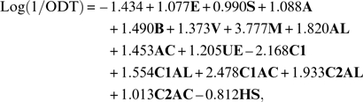
From our preliminary analysis, we excluded the 13 compounds in Table 2, and we assigned indicator variables as follows. M is the variable for the mercaptans and takes the value M = 1 for mercaptans and M = 0 for all other compounds. AL is the variable for aldehydes and takes the value AL = 1 for aldehydes and AL = 0 for all other compounds. AC is the variable for acids and takes the value AC = 1 for acids and AC = 0 for all other compounds. UE is the variable for unsaturated esters and takes the value UE = 1 for unsaturated esters and UE = 0 for all other compounds. Application of equation (1), plus the indicator variables resulted in equation (5) where the 193 compounds are those in Table 1:

(5)

The statistics of equation (5) can be regarded as reasonable, especially because we suggest that the self-consistency of Nagata's data is around 0.66 log unit. Following our previous work (Abraham et al. 2001), we added a term in L² to equation (5), but it led to no improvement in the statistics. Equation (5) appears to be the first equation proposed for the correlation of Nagata's data.

The indicator variables used in equation (5) are not just arbitrary variables used to obtain a better fit to the data; they serve a purpose beyond any increase in fit to the equation. Alarie, Nielsen, et al. (1998) and Alarie, Schaper, et al. (1998) investigated the sensory irritation of mice by airborne chemicals and classed chemicals as acting by a physical mechanism (p) or by a chemical mechanism (c). Compounds that induced sensory irritation by a chemical mechanism were identified through an increase in potency by comparison with that calculated for irritation by a physical mechanism. In essence, this is the same procedure that we have used to identify compounds that are more potent than calculated from equation (4). It was shown that carboxylic acids, aldehydes, and unsaturated esters were more potent than expected, exactly as we have found (Alarie, Nielsen, et al. 1998; Alarie, Schaper, et al. 1998).

Incorporation of other data sets

The ODT values obtained by Cometto-Muñiz and Cain as the C1 data set are in Table 3 (Cometto-Muñiz and Cain 1990, 1991, 1993, 1994; Cometto-Muñiz, Cain, and Abraham 1998; Cometto-Muñiz, Cain, Abraham, et al. 1998). If we omit acids and aldehydes, because of the problem of the necessity for indicator variables, the average difference is 2.129 log units between the Nagata data set and the C1 data set for 30 common compounds. Thus, the Nagata absolute ODT values are lower than the C1 values by a factor of about 100.

Table 3.

Cometto-Muñiz and Cain values (set C1) of ODTs (ppm)

Compound	Log (1/ODT)	Compound	Log (1/ODT)
1-Octene	−2.310	Toluene	−2.190
1-Octyne	−2.130	Ethyl benzene	−1.260
Butanal	−0.477	Propyl benzene	−0.470
Pentanal	−0.699	Isopropylbenzene	−0.033
Hexanal	1.097	Butyl benzene	−0.630
Heptanal	1.523	p-Cymene	−0.121
Octanal	2.398	Pentyl benzene	0.004
2-Pentanone	−0.930	Hexyl benzene	0.190
2-Heptanone	−0.270	Heptyl benzene	0.250
2-Nonanone	0.030	Octyl benzene	0.430
Ethyl acetate	−2.240	Chlorobenzene	−1.110
Propyl acetate	−1.390	Pyridine	−0.110
Butyl acetate	−0.380	α-Pinene	−1.277
sec-Butyl acetate	−0.570	β-Pinene	−1.070
Pentyl acetate	−0.070	(R)-(+)-Limonene	−0.994
Hexyl acetate	0.200	(S)-(−)-Limonene	−0.659
Heptyl acetate	0.010	α-Terpinene	−0.152
Octyl acetate	0.410	γ-Terpinene	−0.992
Decyl acetate	0.500	1,8-Cineole	0.495
Dodecyl acetate	1.360	Linalool	0.022
Formic acid	−0.886	Geraniol	1.070
Butanoic acid	2.444	Menthol	1.660
Hexanoic acid	2.585	β-Phenylethyl alcohol	2.190
Octanoic acid	4.959	Δ-3-Carene	−0.223
Methanol	−3.180
Ethanol	−1.850
1-Propanol	−1.150
2-Propanol	−2.700
1-Butanol	−0.300
2-Butanol	−1.980
2-Methyl-2-propanol	−2.780
1-Pentanol	−0.110
1-Hexanol	0.050
1-Heptanol	1.000
4-Heptanol	−0.910

In order to obtain a combined equation that is based on the Nagata values, we introduced an indicator variable, C1, that would place the C1 data set on the Nagata scale; C1 = 1 for the Cometto-Muñiz and Cain values and C1 = 0 for the Nagata values. We also need indicator variables for the Cometto-Muñiz and Cain C1 data set for carboxylic acids, C1AC, and for aldehydes, C1AL.

More recently, complete concentration–detection (called psychometric) odor functions from which the ODT is obtained have been measured (Cometto-Muñiz and Abraham 2008a, 2008b, 2009a, 2009b, 2010a, 2010b; Cometto-Muñiz et al. 2008). These ODT values, which we denote as set C2, are all much smaller than those in set C1 and approach ODT values for the Nagata data set. The C2 data set is given in Table 4. We can include this data in our ODT analysis by use of an indicator variable for the C2 data set; C2 = 1 for compounds in the set and zero for compounds outside the set. In addition, we need indicator variables for carboxylic acids, C2AC, and for aldehydes, C2AL. If the ODT values in the C2 data set are statistically close to the Nagata data set, we expect the coefficient of C2 to be very small.

Table 4.

Cometto-Muñiz and Abraham values (set C2) of ODTs (ppm)

Compound	Log (1/ODT)	Compound	Log (1/ODT)
Ethanol	0.48	Ethylbenzene	2.22
1-Butanol	2.10	Butylbenzene	2.61
1-Hexanol	2.09	Hexylbenzene	2.36
1-Octanol	2.36	Octylbenzene	1.05
Ethyl acetate	0.61	Propanal	2.70
Butyl acetate	2.37	Butanal	3.33
Hexyl acetate	2.54	Hexanal	3.48
Octyl acetate	1.69	Octanal	3.76
Propanone	0.08	Nonanal	3.27
2-Pentanone	1.00	Helional	3.87
2-Heptanone	2.32	Acetic acid	2.28
2-Nonanone	2.26	Butyric acid	3.58
Toluene	1.10	Hexanoic acid	2.99
		Octanoic acid	3.07

Finally, we hoped to incorporate the set of ODTs for petrochemicals that has been obtained by Hellman and Small (Hellman and Small 1974), again using a standard protocol. Although the ODT values were obtained many years ago, the data set includes several types of compounds not present in the Nagata, C1, and C2 data sets, and so it seemed of interest to see if this set of ODT values could also be scaled to the Nagata set. We simply used the Hellman and Small, HS, data set as such and incorporated a new descriptor in order to adjust the HS set to the Nagata set. The descriptor HS = 1 for the HS set of log (1/ODT) values, see Table 5, and HS = 0 for all other values.

Table 5.

Hellman and Small (set HS) of ODTs (ppm)

Compound	Log (1/ODT)	Compound	Log (1/ODT)
Ethene	−2.42	Dipropylamine	1.70
Propene	−1.35	Diisopropylamine	0.89
Buta-1,3-diene	0.35	Dibutylamine	1.10
Dicyclopentadiene	1.96	Propylenediamine	1.85
5-Ethylidene-2-norbornene	1.70	Ethylene diamine	0.00
1,2-Dichloroethane	−0.78	Methanol	−0.63
Propylene dichloride	0.60	Propan-2-ol	−0.51
Fluorotrichloromethane	−0.70	Butan-1-ol	0.52
Diisopropylether	1.77	2-Methylpropan-1-ol	0.17
Dibutylether	1.16	Butan-2-ol	0.92
Ethylene oxide	−2.42	3-Methylbutan-1-ol	0.92
1,2-Propylene oxide	−1.00	Pentan-1-ol	0.68
1,2-Butylene oxide	1.16	2-Methylbutan-1-ol	1.40
1,4-Dioxane	0.10	Hexan-1-ol	2.00
Propanone	−1.30	2-Methylpentan-1-ol	1.62
Butanone	−0.30	2-Ethylbutan-1-ol	1.16
4-Methylpentan-2-one	1.00	2-Ethylhexan-1-ol	1.13
5-Methylhexan-2-one	1.92	Diisobutyl carbinol	−0.16
Cyclohexanone	0.92	Isodecanol	1.70
2-Methylpent-2-ene-4-one	1.77	2-Butoxyethanol	1.00
Isophorone	0.70	Isobutyl cellosolve	−0.03
2,4-Pentanedione	2.00	Diacetone alcohol	−0.01
Ethyl acetate	−0.80	Methyl ethanolamine	0.00
Propyl acetate	1.30	Dimethylethanolamine	1.82
Isopropyl acetate	0.31	Diethylethanolamine	1.96
Butyl acetate	2.22	Toluene	0.77
Isobutyl acetate	0.46	Isopropylbenzene	2.10
2-Ethylhexyl acetate	1.00	Styrene	1.30
Vinyl acetate	0.92	α-Methylstyrene	1.28
2-Methoxyethyl acetate	0.47	Styrene oxide	1.20
2-Ethoxyethylacetate	1.25	Acetophenone	0.52
Butyl cellosolve acetate	0.96	1,3-Dioxolane	−1.23
Ethylene diacetate	1.03	2-Methylpyridine	1.85
Isopropylamine	0.68	2-Methyl-5-ethylpyridine	2.22
Butylamine	1.10	Morpholine	2.00
Diethylamine	1.70	N-Ethylmorpholine	1.10

For the combined sets of data, the coefficient of C2 was very small, at −0.020, rather as we had expected, and so this descriptor was dropped to yield the final general equation (6). We summarize the various indicator variables in Table 6:

Table 6.

The indicator variables used in equation (6)

Symbol	Variable
M	Mercaptans
AL	Aldehydes
AC	Carboxylic acids
UE	Unsaturated esters
C1	The Cometto-Muñiz and Cain data set
C1AL	Aldehydes in the Cometto-Muñiz and Cain data set
C1AC	Carboxylic acids in the Cometto-Muñiz and Cain data set
C2	The Cometto-Muñiz and Abraham data set
C2AL	Aldehydes in the Cometto-Muñiz and Abraham data set
C2AC	Carboxylic acids in the Cometto-Muñiz and Abraham data set
HS	The Hellman and Small data set

(6)

The statistics of equation (6) are just as good as those of equation (5), even though we now have no less than 353 data points. We include the leave-one-out statistics PRESS and Q² so that we can calculate the predictive standard deviation, PSD, from PRESS. The model is fitted without the ith observation, and this fitted model is then used to predict the response, ŷ_(i) at x_i. This is repeated 352 times, so that each observation has been once excluded. The PRESS residuals are defined as e_(i) = y_i − ŷ_(i) and PRESS is given as PRESS = ∑e_(i)². Then Q² = 1 − (PRESS/SST) where SST is the total sum of squares. PSD is defined similarly to SD; the latter is given by SD = √[SSE/(N − 1 – v)] where SSE is the sum of squares of errors and v is the number of independent variables and PSD = √[PRESS/(N − 1 – v)] (Abraham, Acree, et al. 2009). A value of PSD = 0.869 log units is probably as good as one can get, if the self-consistency of Nagata's data is around 0.66 log unit. It is difficult to apply any general method of selection in order to construct a training and a test set for the 353 data points because the latter are ordered into groups. We therefore simply selected every second compound as a training set. This gave a training set of 176 compounds and a test set of 177 compounds. The training set was regressed against the descriptors used in equation (6) to yield an equation very similar to equation (6), with N = 176, R² = 0.791, and SD = 0.794. This training equation was then used to predict values for the remaining 177 compounds in the test set. For the predicted and observed log (1/ODT) values, we found the absolute error = 0.078, the average absolute error = 0.692, the root mean square error = 0.874, and SD = 0.877 log units. The very small absolute error means that there is no bias in the predictions, and the value of SD, very close to PSD = 0.869, suggests that equation (6) can be used to predict further values of log (1/ODT) to around 0.88 log units. We suggest that equation (6) be used in the prediction of further values of log (1/ODT) on the Nagata scale. Of course, only the Nagata indicator variables, M, AL, AC, and UE then need to be considered.

Scaling to the Nagata set

A plot of calculated values of log (1/ODT) on equation (6) against the observed values is shown in Figure 2. The 4 sets of experimental values are randomly distributed around the line of identity, showing that the indicator variables do indeed bring the Cometto-Muñiz and Cain, the Cometto-Muñiz and Abraham, and the Hellman and Small ODTs onto the same scale as the Nagata thresholds. The value of using all 3 sets can be seen by the very wide range of the experimental log (1/ODT) values shown in Figure 2—almost 9 log units. We can also show how the chemical space of the compounds is increased by the addition of the 3 other groups to the Nagata set. We can identify chemical space in terms of the 5 Abraham descriptors in equation (6). A principal component analysis of the values of the 5 descriptors yields 5 orthogonal PCs that contain all the information of the 5 descriptors. The first 2 PCs account for 60% of the total information, and a plot of the scores of PC2 against PC1 will indicate the chemical space in 2 dimensions, see Figure 3. This figure shows how the chemical space of the Nagata data set can be expanded by incorporation of the other 3 data sets.

Figure 2.

A plot of log (1/ODT) calculated on equation (6) against log (1/ODT) observed: ○, Nagata data set; •, the C1 data set; ▴, the C2 data set; and ▪, the HS data set.

Figure 3.

A plot of PC2 against PC1 for all the data points: ○, Nagata data set; •, the C1 data set; ▴, the C2 data set; and ▪, the HS data set.

We investigated the use of a parabolic relationship in L by adding a term in L² to equation (6), but the resulting equation was no better than equation (6). We also investigated an alternative equation, equation (7). The general equation (1) has invariably been used to correlate quantities that refer to transfer from the gas phase to a condensed phase, for example, gas to blood (Abraham et al. 2005), gas to brain (Abraham et al. 2006a), gas to muscle (Abraham et al. 2006b), gas to olive oil (Abraham and Ibrahim 2006) as well as numerous other gas to solvent partitions. The alternative Abraham equation, equation (7), has been used to correlate quantities that refer to transfer from one condensed phase to another, for example, water to solvent partitions. In equation (7), the independent variable, V, is the McGowan volume in units of (cm³ mol⁻¹)/100:

(7)

Although equation (7) usually leads to worse statistics than equation (1) when applied to gas-to-condensed-phase transfers, we thought it useful to apply equation (7) to the entire data set used to construct the general equation (6). The L descriptor in equation (1) is usually obtained experimentally from data on gas chromatographic retention times (Abraham et al. 2004) or can be estimated from fragment-based schemes (Platts et al. 1999; ADME Boxes 2010). However, there is no need even to estimate V because it is specifically defined in terms of atom and bond contributions (Abraham and McGowan 1987). All that is required to calculate V is a knowledge of the molecular formula and a count of the number of bonds, Bn. The latter can be obtained trivially from the algorithm of Abraham (Abraham 1993): Bn = Na − 1 − R where Na is the total number of atoms in the molecule and R is the number of rings. There is thus an advantage of equation (7) over equation (1) in that one less descriptor needs to be determined or estimated. When we applied equation (7) to the 353 ODTs, we obtained equation (8) after leaving out the term in C2 (0.138 ± 0.230):

(8)

Equation (8) is not quite as good as equation (6) but might be useful in cases where the descriptor L is missing. The coefficients of the Abraham descriptors are not the same in equation (8) as in equation (6), because V and L encode somewhat different chemical information. Hence in comparison of coefficients for various gas-to-condensed-phase processes, equation (6) should be used. However, as a practical equation for the prediction of further values of ODTs on the Nagata scale, equation (8) is an alternative to equation (6).

Equations 6 and 8 should lead to predictions of log (1/ODT) to within an SD value of 0.87 or 0.98 log units, respectively. There is already a data base of several thousand volatile compounds for which the descriptors in equations 6 and 8 are available (Abraham 1993; Abraham et al. 2004; ADME Boxes 2010), and hence, log (1/ODT) values can be predicted for these compounds straight away. In addition, it is possible to predict descriptors just from structure (Platts et al. 1999; ADME Boxes 2010) and so in principle a log (1/ODT) value can be predicted for almost any structure. Of course, the same “caveats” with respect to reactive compounds will apply to both equations 6 and 8; these equations have indicator variables for compounds containing specific reactive groups. Hence, the equations cannot be used to predict ODTs for compounds that contain other reactive groups that we have not taken into account. Of course, once log (1/ODT) values are available for a number of compounds with a new reactive group, equations 6 and 8 can be amended by the incorporation of a new indicator variable for the new reactive group. The principal component analysis, the regression equations, and the various calculations were all carried out using Minitab software (Minitab 2003).

In studying thresholds for eye irritation and nasal pungency (2 trigeminal, as opposed to olfactory chemosensory endpoints), we have recently shown that for several homologous series, the potency of the higher members of the series reaches a “cutoff” point where the homologs fail to even reach a detection threshold (Cometto-Muñiz et al. 2005a, 2005b, 2006, 2007a, 2007b; Cometto-Muñiz and Abraham 2008a, 2008b). This cutoff in potency seems not to be due to a physical mechanism such as lack of sufficient concentration to elicit a response but rather to a chemical mechanism possibly connected with the size of the irritant and the size of the irritation, that is, nociceptive receptor(s) (Peier et al. 2002; Julius 2005; Macpherson et al. 2005; Bautista et al. 2006; Owsianik et al. 2006; Bandell et al. 2007). In terms of olfactory detection thresholds, the existence and basis for a cutoff point has not been yet systematically investigated as with trigeminal thresholds. If it turns out that there is a similar cutoff point for ODTs, then none of the equations we have constructed will correctly predict ODTs for higher members of homologous series. Because, at least for eye irritation thresholds, the cutoff point is not reached until the chain length is about 11–13 carbon atoms for a simple aliphatic homologous series, this may not restrict the application of our equations for odor thresholds very much. However, it is another caveat to keep in mind.

Comparison of odor threshold data and chemesthetic threshold data

Whenever applied to odor threshold data, the Abraham equation fits less well than when applied to chemesthetic threshold data. The R² for the odor data equation (6) is 0.759, whereas the R² for nasal pungency thresholds is 0.955 (Abraham et al. 2001). This suggests that the mechanism that underlies odor detection is more complex than the mechanism that underlies chemesthetic detection. For olfaction, the variety of perceived qualities and the size of the family of genes needed to support transduction of that variety exceeds that for chemesthesis by an order of magnitude or more (Bandell et al. 2007). The large difference in complexity could easily indicate the need for more, or for different, parameters for olfaction. Without incorporation of such parameters, whatever their nature, the LFER would in principle lack some level of precision.

Another explanation that rests upon a systematic difference in transduction between olfaction and chemesthesis seems just as plausible and has important implications for the nature of detection. The difference in transduction can be seen in the psychometric functions for olfactory and chemesthetic detection. Figure 4 shows functions for the detection of 2,2,4-trimethyl-1,3-pentanediol diisobutyrate and ethanol (Cain et al. 2005). The odor of each increases less sharply than does its feel in the nose or eyes. A difference in sharpness has occurred for every material studied for both outcomes (Cain et al. 2007; Cain and Schmidt 2009). It is typically in excess of 1–2 log units, see Figure 4. It follows that the uncertainty in any estimate of an odor threshold will be much larger than the uncertainty of an estimate of a chemesthetic threshold compare SD = 0.27 log units for our equation for nasal pungency thresholds (Abraham et al. 2001) with SD = 0.82 log units in equation (6). The shallower functions for olfaction represent a systematic difference from chemesthesis. Although this shows itself in a probabilistic measure, such as the SD, it actually represents a systematic difference in how the 2 modalities function. In this respect, it does not derive from more instability in olfaction, just a shallower input–output function. The substantive meaning is that the Abraham equation predicts each outcome approximately as well.

Figure 4.

Psychometric functions for chemosensory detection of the plasticizer 2,2,4-trimethyl-1,3-pentanediol diisobutyrate (TXIB) and ethanol. Top panel shows detection of odor, the middle and bottom panels show detection of feel or irritation. The measurement of feel in the nose entails localization of which of the 2 nostrils felt the stimulus. Vertical dashed lines show saturated vapor concentrations (Cain et al. 2005).

When previously addressed, and on the premise that the equation fit chemesthesis relatively better, it made sense to consider that the 2 modalities differed in terms of the specificity of their determining factors. In light of this new interpretation, they need not differ. The fit of the Abraham equation to olfaction, as examined here, might be as good as it is possible to get. If true, then a linear combination of solvation properties might explain all of olfactory sensitivity except for the groups of chemicals that require index variables. Nevertheless, insofar as the index variables are actually constant per group, then the solvation properties would hold within the group.

Funding

The work described in this article was supported by research grant numbers R01 DC002741, R01 DC005003, and R01 DC56602 from the National Institute on Deafness and Other Communication Disorders and National Institutes of Health.

References

- Abraham MH. Scales of hydrogen bonding: their construction and application to physicochemical and biochemical processes. Chem Soc Rev. 1993;22:73–83. [Google Scholar]
- Abraham MH, Acree WE, Jr., Cometto-Muñiz JE. Partition of compounds from water and air into amides. New J Chem. 2009;33:2034–2043. doi: 10.1039/b907118k. [DOI] [PMC free article] [PubMed] [Google Scholar]
- Abraham MH, Acree WE, Jr., Leo AJ, Hoekman D. The partition of compounds from water and from air into wet and dry ketones. New J Chem. 2009;33:568–573. doi: 10.1039/b907118k. [DOI] [PMC free article] [PubMed] [Google Scholar]
- Abraham MH, Andonian-Haftvan J, Cometto-Muñiz JE, Cain WS. An analysis of nasal irritation thresholds using a new solvation equation. Fundam Appl Toxicol. 1996;31:71–76. doi: 10.1006/faat.1996.0077. [DOI] [PubMed] [Google Scholar]
- Abraham MH, Gola JRM, Cometto-Muñiz JE, Cain WS. The correlation and prediction of VOC thresholds for nasal pungency, eye irritation and odour in humans. Indoor Built Environ. 2001;10:252–257. [Google Scholar]
- Abraham MH, Gola JRM, Cometto-Muñiz JE, Cain WS. A model for odor thresholds. Chem Senses. 2002;27:95–104. doi: 10.1093/chemse/27.2.95. [DOI] [PubMed] [Google Scholar]
- Abraham MH, Ibrahim A. Gas to olive oil partition coefficients: a linear free energy analysis. J Chem Inf Model. 2006;46:1735–1741. doi: 10.1021/ci060047p. [DOI] [PubMed] [Google Scholar]
- Abraham MH, Ibrahim A, Acree WE., Jr. Air-to blood distribution of volatile organic compounds: a linear free energy analysis. Chem Res Toxicol. 2005;18:904–911. doi: 10.1021/tx050066d. [DOI] [PubMed] [Google Scholar]
- Abraham MH, Ibrahim A, Acree WE., Jr. Air to brain, blood to brain and plasma to brain distribution of volatile organic compounds: linear free energy analysis. Eur J Med Chem. 2006a;41:494–502. doi: 10.1016/j.ejmech.2006.01.004. [DOI] [PubMed] [Google Scholar]
- Abraham MH, Ibrahim A, Acree WE., Jr. Air to muscle, and blood/plasma to muscle, distribution of volatile organic compounds and drugs: linear free energy analyses. Chem Res Toxicol. 2006b;19:801–808. doi: 10.1021/tx050337k. [DOI] [PubMed] [Google Scholar]
- Abraham MH, Ibrahim A, Zissimos AM. The determination of sets of solute descriptors from chromatographic measurements. J Chromatogr A. 2004;1037:29–47. doi: 10.1016/j.chroma.2003.12.004. [DOI] [PubMed] [Google Scholar]
- Abraham MH, Kumarsingh R, Cometto-Muñiz JE, Cain WS. Draize eye scores and eye irritation thresholds in man can be combined into one quantitative structure-activity relationship. Toxicol In Vitro. 1998;12:403–408. doi: 10.1016/s0887-2333(98)00010-1. [DOI] [PubMed] [Google Scholar]
- Abraham MH, Kumarsingh R, Cometto-Muñiz JE, Cain WS, Roses M, Bosch E, Diaz ML. The determination of solvation descriptors for terpenes, and the prediction of nasal pungency thresholds. J Chem Soc Perkin Trans 2. 1998:2405–2411. [Google Scholar]
- Abraham MH, McGowan JC. The use of characteristic volumes to measure cavity terms in reversed-phase liquid chromatography. Chromatographia. 1987;23:243–246. [Google Scholar]
- ADME Suite. 2010. Version 5.0. Toronto (Canada): Advanced Chemistry Development, Inc [Google Scholar]
- Alarie Y, Nielsen GD, Abraham MH. A theoretical approach to the Ferguson principle and its use with non-reactive and reactive airborne chemicals. Pharmacol Toxicol. 1998;83:270–279. doi: 10.1111/j.1600-0773.1998.tb01481.x. [DOI] [PubMed] [Google Scholar]
- Alarie Y, Schaper M, Nielsen GD, Abraham MH. Structure-activity relationships of volatile organic chemicals as sensory irritants. Arch Toxicol. 1998;72:125–140. doi: 10.1007/s002040050479. [DOI] [PubMed] [Google Scholar]
- American Industrial Hygiene Association (AIHA) Odor thresholds for chemicals with established occupational standards. Akron (NY): AIHA; 1989. [Google Scholar]
- Bandell M, Macpherson LJ, Patapoutian A. From chills to chilis: mechanisms for thermosensation and chemesthesis via thermoTRPs. Curr Opin Neurobiol. 2007;17:490–497. doi: 10.1016/j.conb.2007.07.014. [DOI] [PMC free article] [PubMed] [Google Scholar]
- Bautista DM, Jordt SE, Nikai T, Tsuruda PR, Read AJ, Poblete J, Yamoah EN, Basbaum AI, Julius D. TRPA1 mediates the inflammatory actions of environmental irritants and proalgesic agents. Cell. 2006;124:1269–1282. doi: 10.1016/j.cell.2006.02.023. [DOI] [PubMed] [Google Scholar]
- Cain WS. Testing olfaction in clinical setting. Ear Nose Throat J. 1989;68:322–328. [PubMed] [Google Scholar]
- Cain WS, de Wijk RA, Jalowayski AA, Pilla Caminha G, Schmidt R. Odor and chemesthesis from brief exposures to TXIB. Indoor Air. 2005;15:445–457. doi: 10.1111/j.1600-0668.2005.00390.x. [DOI] [PubMed] [Google Scholar]
- Cain WS, Schmidt R. Can we trust odor databases? Example of t- and n-butyl acetate. Atmos Environ. 2009;43:2591–2601. [Google Scholar]
- Cain WS, Schmidt R, Jalowayski AA. Odor and chemesthesis from exposures to glutaraldehyde vapor. Int Arch Occup Environ Health. 2007;80:721–731. doi: 10.1007/s00420-007-0185-0. [DOI] [PubMed] [Google Scholar]
- Cometto-Muñiz JE. Physicochemical basis for odor and irritation potency of VOCs. In: Spengler JD, Samet J, McCarthy JF, editors. Indoor air quality handbook. New York: Mcgraw-Hill; 2001. pp. 20.1–20.21. [Google Scholar]
- Cometto-Muñiz JE, Abraham MH. Human olfactory detection of homologous n-alcohols measured via concentration-response functions. Pharmacol Biochem Behav. 2008a;89:279–291. doi: 10.1016/j.pbb.2007.12.023. [DOI] [PMC free article] [PubMed] [Google Scholar]
- Cometto-Muñiz JE, Abraham MH. A cut-off in ocular chemesthesis from vapors of homologous alkylbenzenes and 2-ketones as revealed by concentration-detection functions. Toxicol Appl Pharmacol. 2008b;230:298–303. doi: 10.1016/j.taap.2008.03.011. [DOI] [PMC free article] [PubMed] [Google Scholar]
- Cometto-Muñiz JE, Abraham MH. Olfactory detectability of homologous n-alkylbenzenes as reflected by concentration-detection functions in humans. Neuroscience. 2009a;161:236–248. doi: 10.1016/j.neuroscience.2009.03.029. [DOI] [PMC free article] [PubMed] [Google Scholar]
- Cometto-Muñiz JE, Abraham MH. Olfactory psychometric functions for homologous 2-ketones. Behav Brain Res. 2009b;201:207–215. doi: 10.1016/j.bbr.2009.02.014. [DOI] [PMC free article] [PubMed] [Google Scholar]
- Cometto-Muñiz JE, Abraham MH. Odor detection by humans of lineal aliphatic aldehydes and helional as gauged by dose-response functions. Chem Senses. 2010a;35:289–299. doi: 10.1093/chemse/bjq018. [DOI] [PMC free article] [PubMed] [Google Scholar]
- Cometto-Muñiz JE, Abraham MH. Structure-activity relationships on the odor detectability of homologous carboxylic acids by humans. Exp Brain Res. 2010b;207:75–84. doi: 10.1007/s00221-010-2430-0. [DOI] [PMC free article] [PubMed] [Google Scholar]
- Cometto-Muñiz JE, Cain WS. Thresholds for odor and nasal pungency. Physiol Behav. 1990;48:719–725. doi: 10.1016/0031-9384(90)90217-r. [DOI] [PubMed] [Google Scholar]
- Cometto-Muñiz JE, Cain WS. Nasal pungency, odor, and eye irritation thresholds for homologous acetates. Pharmacol Biochem Behav. 1991;39:983–989. doi: 10.1016/0091-3057(91)90063-8. [DOI] [PubMed] [Google Scholar]
- Cometto-Muñiz JE, Cain WS. Efficacy of volatile organic compounds in evoking nasal pungency and odor. Arch Environ Health. 1993;48:309–314. doi: 10.1080/00039896.1993.9936719. [DOI] [PubMed] [Google Scholar]
- Cometto-Muñiz JE, Cain WS. Sensory reactions of nasal pungency and odor to volatile organic compounds. The alkylbenzenes. Am Ind Hyg Assoc J. 1994;55:811–817. doi: 10.1080/15428119491018529. [DOI] [PubMed] [Google Scholar]
- Cometto-Muñiz JE, Cain WS, Abraham MH. Nasal pungency and odor of homologous aldehydes and carboxylic acids. Exp Brain Res. 1998;118:180–188. doi: 10.1007/s002210050270. [DOI] [PubMed] [Google Scholar]
- Cometto-Muñiz JE, Cain WS, Abraham MH. Determinants for nasal trigeminal detection of volatile organic compounds. Chem Senses. 2005a;30:627–642. doi: 10.1093/chemse/bji056. [DOI] [PubMed] [Google Scholar]
- Cometto-Muñiz JE, Cain WS, Abraham MH. Molecular restrictions for human eye irritation by chemical vapors. Toxicol Appl Pharmacol. 2005b;207:232–243. doi: 10.1016/j.taap.2005.02.004. [DOI] [PubMed] [Google Scholar]
- Cometto-Muñiz JE, Cain WS, Abraham MH, Gil-Lostes J. Concentration-detection functions for the odor of homologous n-acetate esters. Physiol Behav. 2008;95:658–667. doi: 10.1016/j.physbeh.2008.09.021. [DOI] [PMC free article] [PubMed] [Google Scholar]
- Cometto-Muñiz JE, Cain WS, Abraham MH, Kumarsingh R. Trigeminal and olfactory chemosensory impact of selected terpenes. Pharmacol Biochem Behav. 1998;60:765–770. doi: 10.1016/s0091-3057(98)00054-9. [DOI] [PubMed] [Google Scholar]
- Cometto-Muñiz JE, Cain WS, Abraham MH, Sánchez-Moreno R. Chemical boundaries for detection of eye irritation in humans from homologous vapors. Toxicol Sci. 2006;91:600–609. doi: 10.1093/toxsci/kfj157. [DOI] [PubMed] [Google Scholar]
- Cometto-Muñiz JE, Cain WS, Abraham MH, Sánchez-Moreno R. Concentration-detection functions for eye irritation evoked by homologous n-alcohols and acetates approaching a cut-off point. Exp Brain Res. 2007a;182:71–79. doi: 10.1007/s00221-007-0966-4. [DOI] [PubMed] [Google Scholar]
- Cometto-Muñiz JE, Cain WS, Abraham MH, Sánchez-Moreno R. Cutoff in detection of eye irritation from vapors of homologous carboxylic acids and aliphatic aldehydes. Neuroscience. 2007b;145:1130–1137. doi: 10.1016/j.neuroscience.2006.12.032. [DOI] [PMC free article] [PubMed] [Google Scholar]
- Devos M, Patte F, Rouault J, Laffort P, Van Gemert LJ. Standardized human olfactory thresholds. Oxford: IRL Press at Oxford University Press; 1990. [Google Scholar]
- Dube MF, Green CR. Methods of collection of smoke for analytical purposes. Rec Adv Tob Sci. 1982;8:42–102. [Google Scholar]
- Environmental Protection Agency (US EPA) Reference guide to odor thresholds for hazardous air pollutants listed in the clean air act amendments of 1990. 1992. EPA600/R-92/047, March 1992. Washington (DC): U.S. Environmental Protection Agency. [Google Scholar]
- Hellman TM, Small FH. Characterization of the odor properties of 101 petrochemicals using sensory methods. J Air Pollut Control Assoc. 1974;24:979–982. doi: 10.1080/00022470.1974.10470005. [DOI] [PubMed] [Google Scholar]
- Iwasaki Y. In: Odor measurement review. Tokyo (Japan): Office of Odor, Noise and Vibration, Environmental Management Bureau, Ministry of Environment; 2003. The history of odor measurement in Japan and triangle odor bag method; pp. 37–47. [Google Scholar]
- Julius D. From peppers to peppermints: natural products as probes of the pain pathway. Harvey Lect. 2005;101:89–115. [PubMed] [Google Scholar]
- Macpherson LJ, Geierstanger BH, Viswanath V, Bandell M, Eid SR, Hwang S, Patapoutian A. The pungency of garlic: activation of TRPA1 and TRPV1 in response to allicin. Curr Biol. 2005;15:929–934. doi: 10.1016/j.cub.2005.04.018. [DOI] [PubMed] [Google Scholar]
- Minitab . Version 14. State College (PA): Minitab Inc; 2003. [Google Scholar]
- Nagata Y. Odor measurement review. Tokyo (Japan): Office of Odor, Noise and Vibration, Environmental Management Bureau, Ministry of Environment; 2003. Measurement of odor threshold by triangle odor bag method; pp. 118–127. [Google Scholar]
- Owsianik G, D'Hoedt D, Voets T, Nilius B. Structure-function relationship of the TRP channel superfamily. Rev Physiol Biochem Pharmacol. 2006;156:61–90. [PubMed] [Google Scholar]
- Peier AM, Moqrich A, Hergarden AC, Reeve AJ, Andersson DA, Story GM, Earley TJ, Dragoni I, McIntyre P, Bevan S, et al. A TRP channel that senses cold stimuli and menthol. Cell. 2002;108:705–715. doi: 10.1016/s0092-8674(02)00652-9. [DOI] [PubMed] [Google Scholar]
- Pierce JD, Doty RL, Amoore JE. Analysis of position of trial sequence and type of diluent on the detection threshold for phenyl ethyl alcohol using a single staircase method. Percept Mot Skills. 1996;82:451–458. doi: 10.2466/pms.1996.82.2.451. [DOI] [PubMed] [Google Scholar]
- Platts JA, Butina D, Abraham MH, Hersey A. Estimation of molecular linear free energy relation descriptors using a group contribution approach. J Chem Inf Comp Sci. 1999;39:835–845. doi: 10.1021/ci990427t. [DOI] [PubMed] [Google Scholar]
- Schmidt R, Cain WS. 2006. The credibility of measured odor thresholds. Presented at the 28th Annual Meeting of the Association for Chemoreception Sciences; 2006 April 28. Sarasota (FL): AChemS. [Google Scholar]
- van Gemert LJ. Utrecht (the Netherlands): Oliemans Punter & Partners BV; 2003. Odour thresholds. Compilations of odour threshold values in air, water and other media. [Google Scholar]