Modeling of Bias for the Analysis of Receptor Signaling in Biochemical Systems

Abstract

Ligand bias is a recently introduced concept in the receptor signaling field that underlies innovative strategies for targeted drug design. Ligands, as a consequence of conformational selectivity, produce signaling bias in which some downstream biochemical pathways are favored over others, and this contributes to variability in physiological responsiveness. Though the concept of bias and its implications for receptor signaling have become more important, its working definition in biochemical signaling is sufficiently imprecise as to impede the use of bias as an analytical tool. In this work, we provide a precise mathematical definition for receptor signaling bias using a formalism expressly applied to logistic response functions, models of most physiological behaviors. We show that signaling-response bias of biological processes may be represented by hyperbolae, or more generally as families of bias coordinates that index hyperbolae. Furthermore, we show bias is a property of a parametric mapping of these indexes into vertical strings that reside within a cylinder of stacked Poincare disks and that bias factors representing signaling probabilities are the radial distance of the strings from the cylinder axis. The utility of the formalism is demonstrated with logistic hyperbolic plots, by transducer ratio modeling, and with novel examples of Poincare disk plots of Gi and β-arrestin biased dopamine 2 receptor signaling. Our results provide a platform for categorizing compounds using distance relationships in the Poincare disk, indicate that signaling bias is a relatively common phenomenon at low ligand concentrations, and suggest that potent partial agonists and signaling pathway modulators may be preferred leads for signal bias-based therapies.

Gprotein-coupled receptors (GPCRs) signal through multiple pathways that are regulated by G proteins andβ-arrestins.^1,2 Many of these signaling pathways respond selectively to ligands that are able to stabilize preferred subsets of receptor conformations.^3,4 As a result of conformational heterogeneity, small differences in ligand structure can dramatically shift signaling toward one response pathway and away from another.⁵ The ability of an agonist–receptor pair to produce a quantitative response, measured as efficacy, has been historically modeled by a transducer ratio parameter reflecting the total receptor concentration and the transduction of the agonist–receptor complex into a pharmacological response.⁶ Potent ligands having low transducer ratios may not be efficacious, and conversely, efficacious responses precipitated by large transducer ratios do not necessarily require potent ligands. Because ligand potencies and their associated transducer ratios can vary widely, a signaling bias may result in which different ligands produce variable degrees of response in a single pathway or a single ligand displays large differences in efficacy between two independent signaling pathways.⁷

A comprehensive review of qualitative and quantitative strategies for assessing ligand bias is found in ref (8). The available approaches similarly address bias within the confines of experiment and attempt to define it observationally or numerically, by data trends or bias factors, as a property that arises from the signaling paradigm. In contrast, an axiomatic formalism for bias could be developed in a manner that is independent of experiment and subsequently applied to a particular signaling paradigm. We believe that this latter approach allows a broader treatment of signaling bias and provides a more fundamental development and conceptual understanding of bias-dependent factors. Applying this strategy to logistic (sigmoid) response functions representative of most biological processes,⁶ we present a comprehensive, simple formalism for qualitative and quantitative signaling bias comparisons. In this formulation, hyperbolae represent the comparative responses of test ligands, and signaling biases are described by mappings of bias coordinates representing the hyperbolae from the unit square to a stack of Poincare unit disks. Bias factors are simple consequences of the map and the novel distance metric of the disk, and the distance between bias coordinates in the disk provides a quantitative means of characterizing and sorting ligands. Our analysis of comparative signaling bias, which can be applied to many signal transduction systems, was developed with G protein-coupled receptors in mind, and we illustrate the approach and its utility using dopamine 2 receptor signaling.

Materials and Methods

Preparation of Theoretical Curves

Equations for the different bias models were added to the library of nonlinear equations in GraphPad Prism 4.0 (GraphPad Software, La Jolla, CA) using the user supplied equations option. Graphs were then prepared under the “generate theoretical curves” option of the analysis menu. Graphs illustrating mappings to the unit disk were prepared using Prism 4.0.

Cell Culture and Transient Transfections

HEK-293T cells (ATCC, Manassas, VA) were cultured in DMEM supplemented with 10% FBS (Sigma, St. Louis, MO) and seeded into a six-well plate at a density of 500000 cells/well. Twenty-four hours later, the cells were transfected with calcium phosphate. Twenty-four hours post-transfection, the cells were split onto white 96-well clear bottom plates (Corning, Lowell, MA) in phenol-free MEM (Gibco, Carlsbad, CA) supplemented with 2% FBS, 2 mM l-glutamine, and 0.05 mg/mL gentamicin. BRET and GloSensor experiments were conducted 24 h after the cells had been plated onto the 96-well plates. For GRK2 overexpression experiments, the cells were transiently transfected alongside BRET and GloSensor assays without GRK2 overexpression. For pertussis toxin (PTX) treatment, the cells were treated 6–8 h after being plated with 200 ng/μL PTX (Sigma) in phenol-free MEM supplemented with 2% FBS, 2 mM l-glutamine, and 0.05 mg/mL gentamicin.

Recruitment of β-Arrestin 2 by BRET

Bioluminescent resonance energy transfer (BRET) assays were performed as described by Masri et al.,¹⁵ with minor modifications. Briefly, mD_2LR-RLuc (mouse dopamine 2 long receptor-Renilla luciferase) was expressed with a saturating concentration of β-arrestin 2-EYFP. Coelenterazine-h (Promega, Madison, WI), at 5 μM, was added to the cells in PBS with calcium and magnesium, followed 5 min later by dose responses of quinpirole (Sigma) or terguride. The ratio of EYFP emission (515–555 nm) to RLuc emission (465–505 nm) was measured using a Mithras LB940 instrument with Mikrowin 2000 (Berthold Technologies, Oak Ridge, TN). The BRET ratios derived were normalized to the maximal quinpirole response on mD_2LR-RLuc.

Measurement of cAMP by GloSensor

HEK-293T cells were transfected with the GloSensor construct (Promega) and mD_2LR. On the day of the experiment, cells were washed in HBSS (Gibco), 25 μL of 25 mM luciferin (Gold Biotechnology, St. Louis, MO) in HBSS was added to each well, and the plates were incubated at room temperature in the dark for 2 h. Following incubation, the luciferin was aspirated, and 80 μL of HBSS was added, followed by dose–response curves of quinpirole. Five minutes after addition of drug, isoproterenol was added at a concentration of 10^–7 M to stimulate the accumulation of cAMP, and the level of accumulation was read 5 min later. Luminescence generated from the GloSensor construct was measured with a Mithras LB940 instrument with Mikrowin 2000. All curves generated were normalized to the maximal response of isoproterenol to control for differences in expression between experiments; the data were then normalized to the maximal response of inhibition of the isoproterenol response by quinpirole.

Theoretical Calculations

Form of the Bias Function B₁₂^a

Conjugate Relationships

For bounded, continuous functions f and g over the interval (c₁, c₂), f(c), g(c) ≥ 0, the bias function is defined as . Note that for relationships of the form , “a” can be said to be conjugate to “b” when it has the same form: . Therefore, when is defined, then B₁₂^a is conjugate to and

Functions f and g Are Chosen as Rectangular Hyperbolae⁹ with Different Hill Coefficients

For unequal Hill coefficients (j ≠ j′), set

Then the bias B₁₂^a, which equals becomes

B₁₂^a in Terms of Conjugate Variables B₀ and B_∞

Important conjugate relationships we will employ to express bias B₁₂^a involving parameters ρ and η are:

In terms of B₀,

Employing the definition of the inner product of two vectors, (a₁,b₁)·(a₂,b₂) = a₁a₂ + b₁b₂, and the change of variable

B₁₂^a in Terms of B₀ and B_∞ for Equal Hill Coefficients

In this case, α = 1 and the bias has the simple form:

where and .

In Transducer Ratio Format

In terms of transducer ratio τ (defined in ref (6), eq 5), we have the relationships and for EC₅₀, where K_A is the ligand affinity. Transducer ratios for the two response functions are:

Form of the Bias Function B₁₂^b (equal Hill coefficients)

From the derivations given above for equal Hill coefficients:

C_1/2 (Half-Height) Concentration of the Bias Function

Because , the value at which the bias approaches half its final value occurs at y = 1. Therefore,

Bias Viewed as a Parametric Mapping from a Square to a Disk

We will demonstrate that bias factors arise from a parametric mapping (mapping parameter θ_y) of a square defined bybias-coefficient co-ordinates B⃗ = (B₀, B_∞) ≤ (±1,±1) onto a unit disk defined by mapped coordinates B⃗^θ_y = (B₀^θ_y, B_∞), ||B⃗^θ_y|| ≤ 1, and (Poincare disk)¹⁰ distance metric:

Inner Products of Complex Numbers and Vectors

The vector inner product is written in the notation ⟨A⃗·C⃗⟩ = ⟨(a,b)·(c,d)⟩ = ac + bd, and this equals the product of the length of the two vectors, ||A⃗||·||C⃗||, times the cosine of the angle x between them. Thus, and are viewed geometrically as the projection of A⃗ on C⃗ and C⃗ on A⃗. For complex numbers B = B₀ + iB_∞ and the complex product BY̅ is:

The inner product of complex numbers B and Y is written as ⟨B·Y̅⟩ and is defined as the real part of BY̅, Re(BY̅). Importantly,

Because the bias function B₁₂^a is always between −1 and 1, the inner product of B and Y in vector or complex number notation must be between −1 and 1. This suggests how to map the unit square into the unit disk.

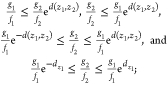
Relationship of Normalized Concentration y to Angles

As y changes from 0 to ∞, goes from 1 to 0, from 0 to 1, and . A plausible relationship is one in which , because their sum is 1; x will range from 0 to . An alternative substitution is y = tan θ_y for . This substitution gives

Families of Hyperbolae

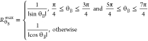
The set of points (B₀ + iB_∞), −1 ≤ B₀, B_∞ ≤ 1 reside in a unit square centered on the origin (0,0). For a fixed angle θ_B from the origin defined by , each co-ordinate point (B₀,B_∞) along the θ_B vector can be represented as αR_θB^max(cos (θ_B) + i sin (θ_B)) = αR_θBe^iθ_B. The point αR_θB^maxe^iθ_B lies on the edge of or inside the unit square for 0 ≤ α ≤ 1 and the following definition for R_θB:

The bias coordinates (B₀,B_∞) in the square along the vector defined by θ_B represent a family of hyperbolae for which tan .

Parametric Map from the Square to the Unit Disk

Define a mapping from the unit square, the points with bias coordinates (B₀,B_∞) = αR_θB^maxe^iθ_B by:

for 0 ≤ α ≤ 1, 0 ≤ θ_B ≤ 2π, and 0 ≤ θ_Y ≤ π/2. This function for a fixed θ_Y (or equivalently for a fixed y) maps every coordinate point (B₀,B_∞) in the unit square to a coordinate point in the unit disk because Re(BY̅) ≤ 1, |e^iθ_B| = 1, and . The term of M(α,θ_B,θ_Y) preserves the orientation between vectors at angle θ_B in the square to vectors at angle θ_B in the disk. The bias magnitude that is between −1 and 1 defines the position of the coordinate along a unit vector in the disk of orientation e^iθ_B.

Projection of the Bias onto Unit Vectors

Because ⟨B·Y̅⟩ can be interpreted as either a projection onto e^iθ_B or e^iθ_Y, we can consider (i) that a point along a fixed direction vector e^iθ_B moves to a different position along e^iθ_B as the parameter θ_Y increases from 0 to . In a second interpretation (ii) we can consider that a point attached to the tip of a vector parallel to e^iθ_Y rotates counterclockwise with e^iθ_Y as θ_Y increases from 0 to , and the length of that vector is the bias and the vector orientation determined by the sign of the bias. Observe that each bias-coefficient coordinate in the unit square is mapped into a stack of disks that form a bias-coordinate cylinder with height of . The particular disk varies with mapping parameter θ_Y.

Distances and Mapping in the Unit Disk and Bias-Cylinder

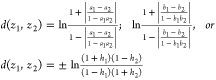
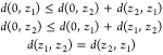
Hyperbolic Distance between Pairs of Complex Points, z₁ and z₂, in the Poincare Disk

This distance is:

For z₁ = (a₁, b₁) and z₂ = (a₂, b₂) this distance is:

For points on the x or y axis, b₁ = b₂ = 0 or a₁ = a₂ = 0,

for h = a or b where the sign is positive if h₁ > h₂ and negative if h₂ > h₁. For,

B₀^m = (B₀, 0) and B_∞^m = (0, B_∞), m = 1, 2:

Distance Preserving Mapping of the Unit Disk in the Complex Plane to Itself

The mapping takes neighborhoods about the point z₁ = c + i·d to neighborhoods about the origin and similarly neighborhoods about the origin to neighborhoods about the point –z₁.¹⁰ For z = a + i·b, this mapping is,

Distance Metric in the θ_y Direction

The metric is because y = tan θ_y. Similar to boundary points, disks near the top of the cylinder are distant from one another even though changes in θ_y may be small.

Relative Probability, Distance, and Bias Factor in the Poincare Disk

Distance from the Origin (zero bias point) and Relative Probability

The distance along the axis to the point R > 0 is:

Define a distance coefficient . For m ≥ 0 and R = this distance is:

Observe that in model B₁₂^a we can set and solve for “m”. Thus,

Therefore, for every unit change in m, the relative probability doubles while the distance along the axis γ_c^m = γ_c.m increases linearly with the change in m. In the Poincare disk the conformal transformations preserve distance relationships, rotations about the center being a special case. We show in Bias Factor Expression β in Heuristic Modeling that the bias factor β is equivalent to a length along the B₀ or B_∞ axis. It can be generalized to the whole disk by rotation for any two points z and z₁; β^L = d(z, z₁), and for

Grouping Bias Coordinates on the Basis of Distance

The distance relationship between the origin and points z₁ and z₂ in the disk satisfies:

Let z be the set of all points in the disk about z₁ such that d(z,z₁) ≤ d_z1. From above, and . Therefore,

indicating all bias coordinates in the neighborhood of z₁ within the distance d_z1 represent response functions g₂ and f₂ having ratios within . For set,

Bias Factor Expression β in Heuristic Modeling⁸

Equiactive Comparison

From Bias Viewed as a Parametric Mapping from a Square to a Disk and Distances and Mapping in the Unit Disk and Bias Cylinder,

For coordinates both associated with vector θ_B,

so that,

with . Identifying E_max with P, EC₅₀ with k, lig with coordinate B₀¹, and ref with coordinate B₀, we obtain the bias factor:

Pharmacological Model

From Bias Viewed as a Parametric Mapping from a Square to a Disk and Distances and Mapping in the Unit Disk and Bias Cylinder,

Therefore, for coordinates with the same θ_B,

so that,

and . Identifying i and j with pathways and ρ₁ and ρ₂ with lig and ref;

Setting β = d(B_∞¹, B_∞) we see that for small transducers for which τ < 1 this result reduces to, which is the result found in ref (8) (within a multiplicative constant). The bias factor defined in ref (8) is appropriate for small transducers. However, for very large transducers in both pathways, this bias factor should in general approach zero, and this is not guaranteed to occur with β defined using . If the reference ligand is unbiased, then ρ_ref = 1 and the bias factor β is d(B_∞¹ ,0) = ln(ρ_lig).

Curve Fitting of Bias Parameters for Bias-Coordinate Distance Determinations

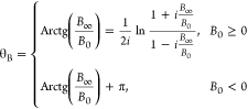
Using the definitions of the arctangent as and hyperbolic arctangent ¹², the above mapping is summarized as a polar co-ordinate transformation. The polar bias coordinates (β,θ_B,θ_Y) are shown below where β is the polar distance and θ_B the polar angle.

The bias co-ordinates in rotated or non-rotated (n = 1 or 0, respectively) complex notation and Euclidean notation are:(x, iy) = bias × e^{i(θ_B–nθ_Y)}, and (x, y) = bias[cos(θ_B – nθ_Y), sin(θ_B – nθ_Y)]. Determining the bias parameters from experiment requires fitting to concentration c and calculating θ_Y, which cannot be expressed as a simple function of c alone. The GraphPad Prism macro below will fit the parameters (B₀,K = log EC₅₀, θ_B) and/or (j, α) against the experimental bias . In most cases, j and α are fixed to 1. The independent variable is X = log(c), and the dependent variable is Y = bias.

Fitting Macro:

• Yc = 10^j(X–K)

• Yα = Yc^(1 – α)

• Yz = 2Yc/([1 + B₀ tan(θ_B)]{1 + [(1 – B₀)/(1 + B₀)]Yα})

• Y₁ = 1/(1 + Yz)

• Y₂ = Yz/(1 + Yz)

• B₁ = {B₀ + [(1 – Yα)/(1 + Yα)]}/{1 + B₀[(1 – Yα)/(1 + Yα)]}

• B₂ = B₀ tan(θ_B)

• Y = B₁Y₁ + B₂Y₂

Results

Overview of Strategy

An analysis of biological signaling bias will be presented in four parts. First, a general bias formalism will be developed with paradigms showing procedures that input response functions and output bias-response functions. Second, the number of candidate paradigmswill be narrowed to two. Third, a particular class of biological response functions will be chosen and processed by each of the bias paradigms for generation of the corresponding bias function. Last, the bias-response functions will be characterized and applied to the analysis of dopamine receptor 2 signaling. Mathematical detail that is not necessary for moving the main discussion forward has been placed in Theoretical Calculations.

Development of Bias Formalism

We now define the properties of a bias response function using a generating function B whose domain includes response functions that are bounded, positive, and continuous. B acts upon paired response functions and by a series of rules creates a corresponding bias function. Specifically, the function B(R₁,R₂) compares the signaling of response functions R₁ and R₂ that represent two processes, A₁ and A₂, with respective inducers c₁ and c₂. R₁ and R₂ are each standardized by normalization using a maximally efficacious inducer, c_1m and c_2m, producing responses E_1m and E_2m, respectively. Thus, the relative response [E_n(c_n)]/E_m of all other inducers (n ≠ m) of either R₁ or R₂ is ≤1.

Because bias suggests preference, a function B(R₁,R₂) for an ordered pair of responses should quantitatively predict an opposite bias exists for the reverse ordered pair, i.e., B(R₁,R₂) = –B(R₂,R₁). Functions with this property are defined as odd as opposed to even functions G with the behavior G(R₁,R₂) = G(R₂,R₁). Additionally, bias implies some difference exists between two responses R₁ and R₂, and a simple relationship to reflect difference is subtraction. This leads to a generating function of the form B(R₂ – R₁) × G(R₁,R₂), where B(R₂ – R₁) is odd and G(R₁,R₂) is even. There are multiple choices for B(R₂ – R₁) and G(R₁,R₂), including those that are combinations of integer powers of R₁ and R₂. Limited to integer powers, and with the straightforward selection of B(R₁,R₂) = R₂ – R₁ (first power in the response functions), there are only two fundamental forms for G(R₁,R₂) (within multiplicative constants) for constructing dimensionless bias functions by B(R₂ – R₁) × G(R₁,R₂).

• (a),
• (b),

with the corresponding bias functions;

• (a),
• (b).

The denominator term in example (a) provides a bounded “probability-like” normalization to B₁₂^a(R₁,R₂). In contrast, the bias B₁₂ (R₁,R₂) depends upon ratios of the response functions and may become problematic in practice when one response is much larger or smaller than the other.

Characteristics of the B₁₂^a Bias Function

B₁₂^a (R₁,R₂) has two characteristic properties related to interpreting the response bias. When the two responses are equal, the bias is 0, and for positive responses, B₁₂ is between −1 and 1. When response R₁ is unlikely and much smaller than response R₂, B₁₂^aasymptotically approaches 1 to indicate this, and conversely, B₁₂approaches −1 when response R₂ is unlikely and much smaller than response R₁. With the normalization for B₁₂^aprovided by R₁ + R₂, the bias B₁₂can be interpreted with a probability formalism where the probability of response R_i(prob R_i), R_i/(R₁ + R₂) (i = 1 or 2), is (1 – B₁₂^a)/2 or (1 + B₁₂)/2 (see the first section of Theoretical Calculations).

Logistic Response Functions

So far, we have not chosen a particular subclass of response functions to plug into the bias formulation from the many positive, bounded, and continuous possibilities. Using ref (6), a plausible candidate is the large cohort of logistic (sigmoid) functions that represent biological processes and are written with Hill parameter j as

I

where 0 ≤ P ≤ 1 as a result of normalization by E_m and k^j equals c^j when a half-maximal response occurs. To couple paired response functions, we define the ratios ρ = P₁/P₂ and η = k₂/k₁ from their defining parameters. Even though the response functions may have different Hill coefficients (j ≠ j′), the following discussion will concentrate on response functions with equal Hill coefficients for the sake of simplicity and because the conclusions carry over to the case of unequal coefficients. It is also no loss of generality to set j equal to 1, because the effect of the exponent, j, in the ratio k^j/c^j can be accounted for by defining k = k^j and c = c^j.

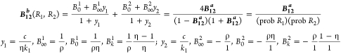
Form of the B₁₂^a Bias Functions

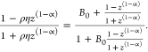
With the selection of logistic response functions described above, the bias function B₁₂^a is a hyperbola that can be conveniently written in one of the three forms shown in eq II. The form (B₀ + B_∞y)/(1 + y) is used for the majority of the discussion and is defined by normalized concentration variable y, baseline B₀, and asymptote B_∞. Parameter B_k = B_∞ – B₀ represents the change in the bias over the interval y = (0,∞).

II

The bias function B₁₂^b (second section of Theoretical Calculations) is the difference of two hyperbolae, has a relatively more complex parametrization than B₁₂, and is related to it by the probabilities of R₁ and R₂ as shown in eq III.

III

For either B₁₂^a or B₁₂, when the response curves have equal EC₅₀ values (i.e., η = 1), the variation parameter B_k identically equals 0 and the bias is constant over the entire concentration range. The concentration at which the bias B₁₂^a will change from its initial value to halfway toward its final value occurs at C_1/2 = [(1 + ρη)/(1 + ρ)]EC₅₀ (see the third section of Theoretical Calculations).

In Figure 1, parameters ρ and η that determine the values of B_∞ and B_k defining bias curves B₁₂^a (panels A, C, and E) also generate the corresponding B₁₂ curves (panels B, D, and F). The curves in the two models are generally similar in appearance, but the range over which the bias varies is always greater in model B₁₂^b (compare especially panels E and F and eq III). Significantly, the additional inflection point (denoting a change in curvature) in the bias graph of Figure 1F results from model B₁₂ requiring a summing of two hyperbolae rather than being represented by a single one, as is B₁₂^a.

Figure 1.

Theoretical bias curves. (A, C, and E) Curves for model B₁₂^a were generated from parameters B_∞ and B_k using GraphPad Prism. Curves shown in panels B, D, and E are the B₁₂ representations of the curves in panels A, C, and E, respectively, using the parameters ρ and η computed from the values of B_∞ and B₀.

Transducer Ratios and Bias Coefficients

Transducer ratios are useful for explaining the variable responses to stimuli that are observed in complex biological systems such as tissue.^6,9As a consequence of how we defined the normalized responses P, we can evaluate the parameters B₀ and B_∞ characterizing the bias functions in terms of transducer ratios⁶ (see the first section of Theoretical Calculations; for a comprehensive discussion of transducer ratios in signaling, see ref (9)). For B₁₂^a, the bias coefficients B₀ and B_∞ in this representation are

IVa

Analogous relationships (eq IVb) can be calculated for the terms describing B₁₂^b or the relationship in eq III applied. The forms of the coefficients as ratios indicate that changes in their magnitudes can become quite large for disparities in pathway transduction or ligand affinities, somewhat limiting their utility for making comparisons.

IVb

From Transducer Ratios to Biased Ligands, Affinity or Efficacy

Natural variables for investigating the behavior of the bias coefficients for B₁₂^a in terms of the transducer ratios are τ₁ and τ₁/τ₂. Panels A–D of Figure 2 show comparative graphs of these relationships for the bias coefficients forming B₁₂ (A and C) and B₁₂^b (B and D). Panels A and B indicate that if one of the transducers such as τ₁ is large, then the bias will approach zero despite some variability in τ₁/τ₂. This occurs because B_∞ in both models asymptotically goes to zero as 1/τ₁. It is also evident in panels C and D from the parametric curves that the baseline bias coefficients B₀ are small whenever the product of ε(τ₁/τ₂) approaches 1. Thus, relatively low concentrations of ligand in this case would have produced limited to no signaling bias. Comparison of panels B and D demonstrates the B₁₂ bias model is subject to wide variations in the zero baseline for changes in ε or τ₁/τ₂. Additionally, comparison of panels A and C indicates that the bias coefficients are more uniformly distributed for changes in parameter τ₁/τ₂ in B₁₂^a. Importantly, the curves in panels C and D show that at relatively low ligand concentrations and very small or large values of ε, B₀ is appreciable and the bias from affinity differences may not be inconsequential and should be considered with pathway efficacy when characterizing drug behavior. The results also suggest that it may be more difficult to develop drugs targeting efficaciously coupled signaling pathways in tissues where the transducer ratios are relatively large but unequal and the concentrations of the drugs are greater than their respective affinities (K_A). One possible developmental strategy for biased ligands would rely upon identifying a compound with a much higher affinity for one of the signaling pathways (very large or small ε in Figure 2C) rather than concentrating solely on differences in efficacy that result from transducer ratios.

Figure 2.

Theoretical curves of bias parameters B_∞ and B₀ as functions of the transducers. Representative curves are shown for model B₁₂^a (A and C) and model B₁₂ (B and D). Curves are parametrized by either τ₁/τ₂ or ε = K_A2/K_A1.

Categorization of Ligands on the Basis of Their Bias Coefficients B₀ and B_∞

Ligand bias coefficients not only define the relative behaviors of dose–response curves but also could potentially represent a means of quantifying differences between ligands; if this is true, what form do the coefficients take in this other role? The following observations present a strategy for answering this question. (1) The set of all pairs of bias coefficients represented in the B₁₂^a model are coordinate points that in aggregate compose a unit square, indicating that the unit square is equivalent to a comprehensive index for addressing response hyperbolae. (2) It is not clear what geometry to apply to the unit square because it lacks rotational symmetry because of the corners, whereas the unit disk has been well characterized in terms of nonstandard geometries for making distance comparisons. Therefore, an improved understanding of signaling bias, including insight into response hyperbolae, bias coefficients, bias coordinates, bias, and bias factors, may evolve from a mapping of points of the unit square to points of the unit disk.

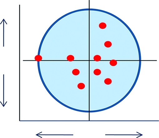
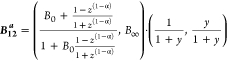
Panels A and B of Figure 3 illustrate an angle-preserving transformation in which every unit square coordinate point B composed of bias coefficients B₀ and B_∞ and lying at position α along a vector at angle θ_B is acted upon by the single vector Y⃗ pointing along parametric angle θ_Y. The effect of Y⃗ on each point B is to map it to a corresponding point in a unit disk lying along the vector at angle θ_B and at a vector position defined by the signaling bias, which is just the term we formerly recognized as (B₀ + B_∞y)/(1 + y) (see the fourth anf fifth sections of Theoretical Calculations). As the parameter θ_Y increases, Y⃗ undergoes a counterclockwise rotation to the angle θ_Y about an axis perpendicular to the disk center. Additionally, the bias generated by B changes, and the mapped point corresponding to B in the disk moves up or down along the θ_B vector (Figure 3C). Alternatively, an observer on the vector Y⃗ can consider it as fixed in direction, and the points corresponding to the mapping of B appear to rotate by θ_Y in the clockwise direction (Figure 3D). This parametric angle preserving mapping of B in the unit square to a point in the unit disk, M(α,θ_B,θ_Y) = ⟨B·Y⃗⟩[(cos θ_B)/|cos θ_B|]e^iθ_B, is described in detail in the fourth and fifth sections of Theoretical Calculations.

Figure 3.

Mappings of the square of bias coordinates bounded by ≤±1 into the Poincare disk. Panels A and B depict the angle preserving nature of the map to the disk that recapitulates the orientation and relative relationships of families of coordinate points that lie along well-defined vectors originating in the center of the square. (C) For an observer sitting on the vector at angle θ_B in the disk, it appears that parametrically mapped points move up or down the length of the vector to a position dependent upon the magnitude and sign of the bias. (D) For an observer sitting on and rotating through angle θ_Y with the mapping vector Y⃗, it appears as if the mapped points B′₀ and B′_inf in the Poincare disk are rotating toward the observer. Additionally, these points are projections of the vertical string that curves about the cylinder axis and that represents the signaling response hyperbola immersed in a three-dimensional space. (E) Cartoon depicting how the string that corresponds to the sigmoid response curve from −1 to 1 (depicted below and at the left) appears in the three-dimensional space of the hyperbolic cylinder. The left-hand cylindrical view depicts the fixed-angle bias interpretation in which the corresponding response string is in a frame where the mapping vector Y⃗ is not only rotating but also changing its length as it rotates (see the accompanying graph below the cylinder at the right for the angular dependence of vector length, which is minimal at π/4). Points are plotted along the fixed vector according to the bias because of the rotation angle of the mapping vector. The right-hand view corresponds to the frame of an observer sitting on the rotation vector that is performing the mapping. In this frame, the disks appear to rotate clockwise as the cylinder and string grow in height with each incremental rotation.

The unit disk can support a non-Euclidean geometry where a familiar Euclidean rule, such as the parallel postulate, is not valid, and distances are computed by a correspondingly unfamiliar metric. Choosing the mapping M(α,θ_B,θ_Y) and a unit disk with a Poincare distance metric results in geometry where the disk boundary is infinitely far from the disk center, where pairs of coordinate points near the boundary can be quite far apart. Also, each θ_Y will map the unit square to a different disk, so that the full map M(α,θ_B,θ_Y) takes the unit square to a cylindrical stack of disks of angular height θ_Y = π/2 (Figure 3E), and where each disk, because Y̅ rotates, is rotated by an angle |dθ_Y| from the disk above or below it. Thus, in aggregate, the mapped-to disks compose a cylinder that is twisted between top and bottom by π/2. Similar to distances computed between points within a disk, the distance between disks near the top becomes very large for small changes in the angular height θ because of a non-Euclidean distance metric that applies to the θ direction (fifth section of Theoretical Calculations). As a consequence, each coordinate point (hyperbola) of the unit square is transformed to a vertical string that rotates by π/2 over its course from the bottom to the top of a three-dimensional twisted cylinder (Figure 3E). The dose–response hyperbolae familiar to pharmacology are two-dimensional projections of these strings, generated by observers rotating with the strings while measuring their magnitudes and directions of displacement (their bias) from the vertical cylinder axis.

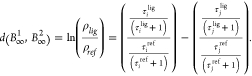
Distance as Bias Factors and Relation to Relative Probability

The hyperbolic distance or length in the Poincare disk between paired, mapped bias coordinates (points) provides a quantitative measure for comparing signaling behaviors and on that basis can be used to sort groups of ligands (fifth and sixth sections of Theoretical Calculations). When one of those coordinates is at the zero bias origin, the hyperbolic length defined by β^L has a straightforward probabilistic interpretation that also applies to any pair of points in the disk. When the ratio of the response functions g and f that compose the bias function is expressed as g/f = 2^m/1, the distance between their corresponding bias coordinate and the origin can be written as β^L = γ_c^m≈ 0.69m (sixth section of Theoretical Calculations). m = 0 is consistent with no bias, and every change in m of 1 doubles the relative probability of g versus f occurring. The coordinate distances between points on the B₀ and B_∞ axes can be written respectively as β^L = ln(ρ₁η₁)/(ρ₂η₂) and β^L = ln(ρ₁/ρ₂), which notably are the bias factors for models described in ref (8) and occur as special consequences of the formalism presented here (seventh section of Theoretical Calculations).

Three Examples of Relative Bias

The examples in Figure 4 will illustrate bias analyses of dopamine D2 receptor signaling using model B₁₂^a and experimental results from our laboratory. Data will be displayed in standard dose–response curve format (projections of cylinder strings onto rectangular grids) and also as string projections onto rotated or fixed-angle Poincare disks oriented perpendicular to the cylindrical axis.

Figure 4.

Bias of compounds at the dopamine 2 receptor in different signaling paradigms. (A–D) Responses are plotted for experimental dose–response data as string projections either in standard dose–response curve format or in either a rotating or fixed-angle Poincare disk representation. (A and B) Bias plots for β-arrestin vs Gi signaling with corresponding parameter and coordinate mapping tables for the agonist quinpirole in the absence or presence of a pathway enhancer (GRK) or inhibitor (pertussis toxin). Distances, β, from the corresponding quinpirole point are provided in the table for nonrotated and rotated coordinates. To provide a comparison of two strategies for calculating bias curves, curves for quinpirole have been calculated from (1) fitting the individual Gi and β-arrestin responses, separately determining the individual P_i and K_i, and then calculating the bias curve (orange curve) or (2) directly fitting the two response ratios (g – f)/(g + f) at different concentrations [∗, ±95% confidence interval (see the eighth section of Theoretical Calculations)]. Additionally, the first and last coordinates plotted for the quinpirole + GRK curve (green) are bounded by closed curves defining neighborhoods of points within a distance of 0.22 [m = 0.32 (see the sixth section of Theoretical Calculations)], or with a <25% difference in the g/f ratio of the bias curves. (C) Plots of the bias of quinpirole and terguride for β-arrestin signaling in the absence and presence of added GRK, a β-arrestin pathway enhancer. (D) Plots representing the bias of different D2 receptor antagonists for inhibiting either the β-arrestin pathway or Gi signaling.

Dopamine 2 Receptor and Signaling Pathway Comparison

Figure 4A shows the system bias between Gi and arrestin signaling for the D2R agonist quinpirole in three dose–response projections (standard, rotated disk, and fixed-angle disk). Bias curves were generated using the maximal response and affinity parameters (P_i and EC₅₀) of the individual signaling curves. To demonstrate an alternative method of generating a bias curve, data for quinpirole bias, (g – f)/(g + f), were directly fit [dashed curve, ●, ±95% confidence interval (see the eighth section of Theoretical Calculations)], and to demonstrate grouping like coordinates with distance, the oval and circular shaded regions at the two ends of the quinpirole + GRK curve (nonrotated disk view) define neighborhoods of points β^L ≤ 0.22 (m = 0.32) of the central coordinates (■ or ●), representing relative probabilities and biases within 25% of those reference coordinates [■ or ● (see the sixth section of Theoretical Calculations)]. Figure 4B displays the unit square bias coordinates, Poincare disk mapped coordinates, transducer ratio parameters, and relative distances (β^L) from the angle equivalent quinpirole coordinates. Quinpirole is a potent D2R ligand that at low concentrations clearly demonstrates greater efficacy for Gi signaling than β-arrestin recruitment in the standard plot, which is reflected also in the Poincare plots by coordinate proximity to the left-side boundary. Quinpirole demonstrates near zero bias at higher concentrations when it loses signaling preference. This suggests that β-arrestin coupling possesses at least a modest transducer ratio; otherwise, the tilt toward Gi signaling bias would remain. The overexpression of GRK shifts the bias curve uniformly upward toward β-arrestin in the standard plot format, suggesting an increase in the β-arrestin transducer that is reflected by increasesin both B₀ and B_∞ (a clockwise rotation of coordinates toward arrestin in the disk model). Pertussis toxin treatment of cells, by noncompetitively inhibiting Gi signaling, markedly drives the bias toward β-arrestin, and this is readily apparent in the fixed-angle disk model by a shift of points to the first quadrant.

Dopamine 2 Receptor Bias in a Single Signaling Pathway

Figure 4C demonstrates an increase in quinpirole bias toward β-arrestin in cells expressing additional GRK compared to β-arrestin in cells expressing normal levels of GRK, a result expected on the basis of mass action for upstream receptor/arrestin modulators.¹³ Additionally, GRK phosphorylation might further enhance the bias by stabilizing receptor states with greater affinity for quinpirole (ε and η increase with increasing affinity). An increased level of expression of GRK is effective in producing a β-arrestin bias at low quinpirole concentrations, and bias coordinates in the disk plot fall closer to the boundary. GRK-induced bias is lost at high quinpirole concentrations, possibly because the transducer for the process is already moderately sized in the absence of additional GRK. Remarkably, terguride bias toward β-arrestin and GRK remains strong at high terguride concentrations even though terguride is more potent than quinpirole with respect to the receptor. The terguride profile is consistent with that of a partial agonist with a relatively small transducer, as observed for morphine-mediated activation of β-arrestin trafficking by the mu opiate receptor.¹⁴

Dopamine 2 Receptor and Pathway Antagonist Comparisons

Data depicted in Figure 4D were based upon D2R studies¹⁵ that investigated whether antagonist signaling bias, evaluated as inhibition of Gi protein signaling versus inhibition of β-arrestin trafficking, differentiates clinically superior neuroleptics from less effective ones. Bias coefficients B₀ and B_∞ for each drug were computed using the affinity and efficacy values listed in Table 1 of ref (15). Not surprisingly, the majority of drugs had little to no bias at high concentrations, indicating a modest transducer ratio for each process. All drugs except olazapine were biased over one to two decades of the displayed concentration range. Aripiprazole stands out, especially in the Poincare fixed disk-angle plot, as the only compound to undergo the transition from a Gi inhibition bias to a β-arrestin inhibition bias, whereas clozapine is unique in being completely β-arrestin biased; its bias coordinate is at the disk boundary and its bias factor correspondingly infinite. Remarkably, all the drugs are biased at low concentrations, and the biases generally disappear as concentrations increase. Apparently, pathway bias is not an uncommon drug property at lower concentrations where affinities play a role in determining transducer ratios, and aripiprazole-like drugs with smaller transducers may form a more likely pool of biased ligands for use at higher concentrations.¹⁶

Discussion

The recent recognition that altering a receptor’s conformational space has physiological consequences has accelerated searches for biased compounds. This study addresses a lack of formalism in receptor bias analysis by characterizing the mathematical relationship between signaling bias and the hyperbolae that commonly describe biological responses. Specifically, we incorporate the response functions into an axiomatic system that defines signaling bias rather than determining the nature of bias on the basis of the responses. Our study shows that (1) coordinates (B₀,B_∞) of paired bias coefficients form a unit square indexing response hyperbolae, (2) the signaling response hyperbolae form groups of families defined by direction vectors centered about (0,0) in the unit square, (3) the bias is the position of the mapped bias coordinate along a direction vector in the unit disk determined by the parametric mapping of the square and ranges between −1 and 1, (4) the bias length or bias factor is the distance to the disk center of the mapped bias coordinate in the Poincare metric, (5) the relative probability between two responses is directly related to the bias factor, and (6) the parametric angles defining the unit square mapping of hyperbolae to the bias (Poincare) cylinder are normalized concentrations that span an angular measure from 0 to π/2. Even though this study investigates hyperbolae describing signaling response bias, it can be applied to the normalized hyperbolae in general that represent biological, pharmacological, or biochemical phenomena.

The B₁₂^a formalism provides a novel and innovative way of considering dose–response data. It provides a qualitative platform for identifying and characterizing ligand and pathway bias using projections of hyperbolic strings for plotting in the Poincare disk or in a standard rectangular format. The formalism also provides for detailed quantitative characterizations of signaling behavior, examples being that the bias factors β in the equiactive and pharmacological models⁸ can be derived as simple consequences of the analysis, and in calculating bias factors, the B₁₂ model appropriately handles large transducer ratios that prove to be problematic for the pharmacological model. Additionally, the Poincare plots show that the bias factor alone is not necessarily a good measure of ligand or signaling differences, because it corresponds to only a radial distance and needs to be associated with an angle or family of curves to reflect the distance relationships of bias coordinates. Thus, a novel application of the formalism may be in drug discovery, where Poincare disk distances and polar bias analysis plots may expedite classifying the behaviors of large numbers of lead compounds in SAR analysis.

Our data indicate that signaling bias in drugs is relatively common, occurring frequently at low to moderate concentrations of compounds. Importantly, for ligands with large transducer ratios for both response pathways, good agonists, for example, there is essentially zero signaling bias at high concentrations. This bias is predominantly lost at high ligand concentrations because in many instances transducers reflect the presence of spare receptors for the pathways. While we do not suggest that developing biased compounds with large transducers is not possible, our results suggest that in the search for pharmacological bias it may be expeditious also to consider lead compounds with low to modest transducer ratios such as partial agonists, to consider the consequences that many drugs are biased when utilized at concentrations below or near the K_A, and to encourage approaches that modify transducers for selected responses using pathway or receptor modulators that act independently of the primary ligand.

Funding Statement

National Institutes of Health, United States

References

- Drake M. T.; Violin J. D.; Whalen E. J.; Wisler J. W.; Shenoy S. K.; Lefkowitz R. J. (2008) β-Arrestin-biased agonism at the β2-adrenergic receptor. J. Biol. Chem. 283, 5669–5676. [DOI] [PubMed] [Google Scholar]
- Rajagopal K.; Whalen E. J.; Violin J. D.; Stiber J. A.; Rosenberg P. B.; Premont R. T.; Coffman T. M.; Rockman H. A.; Lefkowitz R. J. (2006) β-Arrestin2-mediated inotropic effects of the angiotensin II type 1A receptor in isolated cardiac myocytes. Proc. Natl. Acad. Sci. U.S.A. 103, 16284–16289. [DOI] [PMC free article] [PubMed] [Google Scholar]
- Frielle T.; Daniel K. W.; Caron M. G.; Lefkowitz R. J. (1988) Structural basis of β-adrenergic receptor subtype specificity studied with chimeric β1/β2-adrenergic receptors. Proc. Natl. Acad. Sci. U.S.A. 85, 9494–9498. [DOI] [PMC free article] [PubMed] [Google Scholar]
- Rajagopal S.; Rajagopal K.; Lefkowitz R. J. (2010) Teaching old receptors new tricks: Biasing seven-transmembrane receptors. Nat. Rev. Drug Discovery 9, 373–386. [DOI] [PMC free article] [PubMed] [Google Scholar]
- Whalen E. J.; Rajagopal S.; Lefkowitz R. J. (2011) Therapeutic potential of β-arrestin- and G protein-biased agonists. Trends Mol. Med. 17, 126–139. [DOI] [PMC free article] [PubMed] [Google Scholar]
- Black J. W.; Leff P. (1983) Operational models of pharmacological agonism. Proc. R. Soc. London, Ser. B 220, 141–162. [DOI] [PubMed] [Google Scholar]
- Vaidehi N.; Kenakin T. (2010) The role of conformational ensembles of seven transmembrane receptors in functional selectivity. Curr. Opin. Pharmacol. 10, 775–781. [DOI] [PubMed] [Google Scholar]
- Rajagopal S.; Ahn S.; Rominger D. H.; Gowen-McDonald W.; Lam C. M.; Dewire S. M.; Violin J. D.; Lefkowitz R. J. (2011) Quantifying Ligand Bias at Seven-Transmembrane Receptors. Mol. Pharmacol. 80, 367–377. [DOI] [PMC free article] [PubMed] [Google Scholar]
- Kenakin T. P. (2009) A pharmacology primer: Theory, applications, and methods, 3rd ed., Elsevier Academic Press, Amsterdam. [Google Scholar]
- Nevanlinna R. H., and Paatero V. (1969) Introduction to complex analysis, Addison-Wesley Publishing Co., Reading, MA. [Google Scholar]
- Stanoyevitch A.; Stegenga D. A. (1994) The geometry of Poincare disks. Complex Variable Theory Appl. 24, 249–266. [Google Scholar]
- Gradshteyn I. S., Ryzhik I. M., and Jeffrey A. (2000) Table of integrals, series, and products, 6th ed., Academic Press, San Diego. [Google Scholar]
- Menard L.; Ferguson S. S.; Zhang J.; Lin F. T.; Lefkowitz R. J.; Caron M. G.; Barak L. S. (1997) Synergistic regulation of β2-adrenergic receptor sequestration: Intracellular complement of β-adrenergic receptor kinase and β-arrestin determine kinetics of internalization. Mol. Pharmacol. 51, 800–808. [PubMed] [Google Scholar]
- Bohn L. M.; Dykstra L. A.; Lefkowitz R. J.; Caron M. G.; Barak L. S. (2004) Relative opioid efficacy is determined by the complements of the G protein-coupled receptor desensitization machinery. Mol. Pharmacol. 66, 106–112. [DOI] [PubMed] [Google Scholar]
- Masri B.; Salahpour A.; Didriksen M.; Ghisi V.; Beaulieu J. M.; Gainetdinov R. R.; Caron M. G. (2008) Antagonism of dopamine D2 receptor/β-arrestin 2 interaction is a common property of clinically effective antipsychotics. Proc. Natl. Acad. Sci. U.S.A. 105, 13656–13661. [DOI] [PMC free article] [PubMed] [Google Scholar]
- Allen J. A.; Yost J. M.; Setola V.; Chen X.; Sassano M. F.; Chen M.; Peterson S.; Yadav P. N.; Huang X. P.; Feng B.; Jensen N. H.; Che X.; Bai X.; Frye S. V.; Wetsel W. C.; Caron M. G.; Javitch J. A.; Roth B. L.; Jin J. (2011) Discovery of β-Arrestin-Biased Dopamine D2 Ligands for Probing Signal Transduction Pathways Essential for Antipsychotic Efficacy. Proc. Natl. Acad. Sci. U.S.A. 108, 18488–18493. [DOI] [PMC free article] [PubMed] [Google Scholar]