Phase Ambiguity Correction and Visualization Techniques for Complex-Valued ICA of Group fMRI Data

Abstract

Analysis of functional magnetic resonance imaging (fMRI) data in its native, complex form has been shown to increase the sensitivity both for data-driven techniques, such as independent component analysis (ICA), and for model-driven techniques. The promise of an increase in sensitivity and specificity in clinical studies, provides a powerful motivation for utilizing both the phase and magnitude data; however, the unknown and noisy nature of the phase poses a challenge. In addition, many complex-valued analysis algorithms, such as ICA, suffer from an inherent phase ambiguity, which introduces additional difficulty for group analysis. We present solutions for these issues, which have been among the main reasons phase information has been traditionally discarded, and show their effectiveness when used as part of a complex-valued group ICA algorithm application. The methods we present thus allow the development of new fully complex data-driven and semi-blind methods to process, analyze, and visualize fMRI data.

We first introduce a phase ambiguity correction scheme that can be either applied subsequent to ICA of fMRI data or can be incorporated into the ICA algorithm in the form of prior information to eliminate the need for further processing for phase correction. We also present a Mahalanobis distance-based thresholding method, which incorporates both magnitude and phase information into a single threshold, that can be used to increase the sensitivity in the identification of voxels of interest. This method shows particular promise for identifying voxels with significant susceptibility changes but that are located in low magnitude (i.e. activation) areas. We demonstrate the performance gain of the introduced methods on actual fMRI data.

1. Introduction

Functional magnetic resonance imaging (fMRI) is a technique that provides the opportunity to study brain function non-invasively and is a powerful tool utilized in both research and clinical arenas since the early 90s [1]. FMRI data are natively acquired as complex-valued spatio-temporal images; however, usually only the magnitude images are used for analysis. The phase images are usually discarded, primarily because their unfamiliar and noisy nature poses a challenge for successful study of fMRI [2]. However, recent studies have identified the presence of novel information in the phase, which can be utilized to better understand brain function [3, 4, 5, 6, 7, 8]. One exciting implication of this fact would be increased sensitivity in diagnosis when studying differences in control and patient groups when the phase information is utilized.

Both model-based approaches, such as general linear model (GLM), and data-driven approaches, such as independent component analysis (ICA), can be used for studying complex-valued fMRI data. By using a simple generative model based on linear mixing, ICA can minimize the constraints imposed on the temporal—or the spatial—dimension of the fMRI data, and therefore is particularly attractive for studying paradigms for which reliable models of brain activity are not available. Hence, ICA is particularly promising for the analysis of the phase of the complex-valued fMRI data, since it does not make any strong assumptions about its unfamiliar nature. A number of recent applications of ICA to complex fMRI data have demonstrated the promise of ICA for the analysis of fMRI data in its native complex form [2, 9, 10, 11], but have also underlined the importance of preprocessing and visualization techniques to fully take advantage of the additional information presented by the phase.

Successful application of both the model-based and data-driven approaches for analysis of complex-valued fMRI data requires the development of pre-and post-processing techniques that can help exploit the phase information and therefore improve the usability of these algorithms. In this paper, we introduce a phase ambiguity correction scheme and a Mahalanobis distance-based thresholding method that can significantly help improve the analysis and visualization of complex-valued fMRI data. We show the effectiveness of these methods when used in the analysis of actual fMRI group data using a complex-valued ICA algorithm. The main idea for phase ambiguity correction with some preliminary results were given in [12]. These methods, together with a previously developed complex-valued de-noising algorithm [13, 14], form a successful framework that allows one to utilize the phase information in fMRI data to enhance the sensitivity and specificity of ICA of fMRI studies. Fig. 1, shows the steps of the framework, including the two methods introduced in this paper, and the de-noising method. The phase correction step can be incorporated directly into the ICA step as we discuss in the paper. The Mahalanobis distance-based visualization and de-noising methods can be used for model-based approaches, as well as data-driven ones. The rest of the steps in Fig. 1 are typical steps in the pipeline, such as using PCA for data dimensionality reduction and the use of the MATLAB Toolbox for Statistical Parametric Mapping (SPM)² for motion correction.

Figure 1.

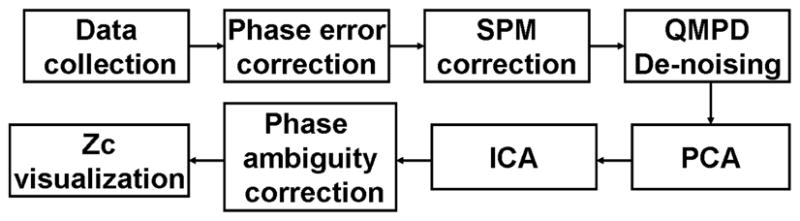
Framework that allows the utilization of the phase along with magnitude at various steps in the implementation of a complex-valued ICA algorithm. Phase ambiguity correction and Mahalanobis distance-based visualization (Z_c) methods are introduced in this paper and the Quality Map Phase De-noising (QMPD) method is introduced in [13, 14].

In Section 3, we describe the phase ambiguity correction scheme that solves the inherent phase scaling ambiguity found in complex-valued data-driven algorithms, such as ICA. The phase ambiguity correction scheme can be either applied subsequent to ICA of fMRI or can be incorporated into the ICA algorithm in the form of prior information—when available—to eliminate the need for further processing.

In Section 4, we describe the novel visualization technique, based on the Mahalanobis distance-based metric, which can be used to identify voxels of interest in complex-valued fMRI images and which provides a single threshold based upon both the phase and magnitude data. In Section 5, we present results of the methods introduced here when applied to actual fMRI group data.

2. Background

2.1. Spatial ICA of Complex-valued fMRI Data

Independent component analysis has emerged as an attractive analysis tool for discovering hidden factors in observed data and has been successfully applied for data analysis in a wide array of applications [15, 16, 17]. Especially in the case of fMRI analysis, it has proven particularly fruitful [18, 19].

In the ICA analysis of fMRI data, we assume independence of spatial brain activations (for spatial ICA), and write the complex ICA model as

$$\mathbf{x}=\mathbf{As}$$

where x is the random vector of observation, A is the mixing matrix and s is the independent source vector. For the volume image data of v voxels and n time points, we can write X = [x₁, x₂, ···, x_v] and S = [s₁, s₂, ···, s_v] where X ∈ ℂ^n×v is formed using the fMRI data such that the kth row is formed by flattening the volume image data of v voxels into a row. The rows of X are indexed as a function of time from one to n and the kth row vector of S is the kth spatial map. The assumed kth mixing column vector of A represents the time course for the kth spatial map.

ICA achieves demixing by estimating a weight matrix W such that ŝ = Wx = PΛs. Here, P, a permutation matrix, represents the permutation ambiguity and Λ, a diagonal matrix, represents the scaling ambiguity of ICA, which has a magnitude and phase term in the complex-valued implementation of ICA.

Thus, spatial ICA finds systematically nonoverlapping, temporally coherent brain regions without constraining the temporal domain. A principal advantage of this approach is its applicability to cognitive paradigms for which detailed a priori models of brain activity are not available. Following its first application by McKeown et al. [19], ICA has been successfully used in a number of exciting fMRI applications, especially in those that have proven challenging with the standard regression-type approaches. These include identification of various signal types (e.g., task-related, transiently task-related, and physiology-related signals) in the spatial or temporal domain, analysis of multisubject fMRI data, incorporation of a priori information to improve the estimates, clinical applications, and for the analysis of complex-valued fMRI data. A comprehensive review of ICA approaches for fMRI data along with main references in the area is given in [20] and in [21].

In spatial ICA, the number of estimated independent components (ICs) correspond to the number of time-points, which in general are in the order of 100s, and for temporal ICA, they correspond to the number of voxels that are much higher. Hence, in both cases, a principal component analysis (PCA) stage traditionally precedes the ICA algorithm that is used to whiten the data and to determine the effective model order. Information theoretic criteria such as Akaike’s information criterion, and the minimum description length (MDL)—or the Bayesian information criterion—arise as natural solutions for determining the effective order of the components as in [22].

ICA requires computation of higher-order statistics in the data, either explicitly as in the approaches based on cumulants, or implicitly through the use of non-linear functions. ICA approaches that rely on non-linear functions to implicitly generate the higher-order statistics to achieve independence offer practical and effective solutions to the ICA problem. As discussed in [23], a number of simple functions from the trigonometric family provide robust and effective solutions for the ICA problem in the complex domain as in the real case, or simple adaptive mechanisms can be employed to estimate the independent components in a deflationary mode as discussed in [24] or simultaneously as in [25].

Since, relative to the magnitude data, there is less known about fMRI data when used in its native complex form, it is desirable to avoid making assumptions such as the circularity of source distributions. A complex random variable (v = v_re + jv_im) is considered circular when its pdf is rotationally invariant, i.e., when the pdf can be written as $p(v_{re},v_{im})=p(\sqrt{v_{re}^2+v_{im}^2})$. Hence, for a circular random variable, the phase is non-informative.

Circularity is a limiting assumption and as we demonstrate with an example, fMRI data exhibits noncircular characteristic in general (see Fig. 2). Since the data are expected to be noncircular, is important to use ICA algorithms that do not make such assumptions as in [26, 24, 25]. However, certain information about the circularity of the data, such as the preprocessing steps used in the scanner, can be incorporated into the algorithm as we discuss in Section 3.

Figure 2.

Complex scatter plot of an estimated motor task-related component of a single subject (see Section 5.1) before and after applying the PCA-based phase ambiguity correction scheme.

3. Phase Ambiguity Correction

In Section 2.1, it was shown how ICA estimates both the sources s and the mixing matrix A up to a permutation and scaling ambiguity. In (1), the relationship, due to the scaling ambiguity, between the estimated and the true value of the sources and the mixing matrix is shown. The phase term in the scaling ambiguity presents additional challenges not observed in real-valued ICA, as in fMRI group studies, the estimated distribution of matching sources across subjects will have different unknown rotations that hinders analysis. Needless to say it is of utmost importance to be able to compare matching estimated components across subjects in fMRI studies. For the ICA model introduced in Section 2.1, we can write

$$\mathbf{x}=\widehat{\mathbf{A}}\widehat{\mathbf{s}}=(\mathbf{A}\mathbf{\Lambda })({\mathbf{\Lambda }}^{-\mathbf{1}}\mathbf{s})$$ (1)

where Λ is the scaling ambiguity diagonal matrix, which has a magnitude and phase term in the complex-valued implementation of ICA if we ignore the permutation ambiguity. This is the reason for the rotation of the 2-D estimated source scatter plots by an arbitrary angle.

In this section, we present two methods that alleviates the phase ambiguity problem and allows for group analysis of estimated ICs. First we introduce an ICA approach that can effectively utilize prior information about the orientation of the raw complex-valued fMRI data to correct the phase rotation of the estimated ICA components. Next, we introduce an approach that can be used to correct for phase rotation in the absence of such prior information and/or when we are interested in using a flexible ICA algorithm, such as one that adaptively estimates the source distributions as in [24]. This second approach in general can be used with any group analysis method (not just ICA), whenever there is phase ambiguity across subjects.

Phase ambiguity affects other applications that use complex-valued data and blind channel identification algorithms are an example [27], therefore methods similar to the ones introduced here could be used to in these areas as well.

3.1. Phase Ambiguity Correction through Prior Information

A common pre-processing technique used in the after the acquisition of complex-valued fMRI data is to re-normalize the data such that most of the power is concentrated in the real part of the complex-valued fMRI signal [28]. This reconstruction technique (second block in Fig. 1) is one of many that are usually used to eliminate collection-related phase errors in raw MRI data, for example, off-resonance effects, radio-frequency pulse imperfections, relaxation effects or discretization artifacts [29, 30]. Such processing makes the visualization easy as all the acquired data then has the same orientation and can be easily added in the case of group analyses. The phase ambiguity correction schemes introduced in this paper are similar to this pre-processing technique, but they are applied to correct the phase ambiguity in the estimated ICs using complex-valued ICA (phase ambiguity correction block in Fig. 1) and not to correct the raw fMRI data phase errors as is done in [28].

Knowledge about the distribution of the fMRI data can be incorporated into the selection of the nonlinear function for the ICA algorithm so that the estimated sources will have the same orientation as the preprocessed data. Here, we present an example of the selection of the nonlinear functions in applications where the fMRI data are preprocessed in the scanner so that most of the power is in the real component [28]. In [23], it has been shown that a number of trigonometric functions and their hyperbolic counterparts can be effectively used for performing ICA, and in [31] it has been noted that by selecting the appropriate function, we can effectively alleviate the phase ambiguity. In Fig. 3, we show the approximate density the use of score function atanh implies (given by exp(−u^*atanhu)), which exactly corresponds to the data that results from the fMRI preprocessing we have described [28]. In the second row of the same figure, we show estimation results of joint approximate diagonalization of eigenmatrices (JADE) [32] and ML with atanh as the score function. In the estimation results, we note that when the direction of the source matches that of the pdf implied by the score function, the shape of the distribution of the estimated components is preserved, i.e., the phase ambiguity that exists for the complex ICA (Λ) is mitigated. Thus, even though the correlations of the magnitude with the original sources are close to unity for both JADE and ML-atanh in this example, the correlation of real and imaginary parts are high (close to unity) only for the ML-atanh estimated sources for which the direction of the source density matches with that of the non-linearity. The red source estimate shows a rotated source estimate whose asymmetry does not match with that of the density model given by atanh. These results were consistent over 100 different realizations of the source distributions.

Figure 3.

Top: Form of pdf implied by the score function atanh; Bottom: Estimation results with ML using atanh score function and JADE for four non-circular sources.

Hence, we can use atanh when such a preprocessing—a desirable form for complex fMRI data—is utilized. The only correction that will then have to be carried out is the sign correction to make sure that most background voxels are around “0”, a post processing step common to real-valued ICA of fMRI [20]. Matching ICs across subjects will have similar orientation and then allow for group analysis

The strength of this scheme lays on identifying prior information that can help in the selection of the non-linear function used in the ICA cost functions. Similar prior information can be used to identify the optimal non-linearities in fMRI data with different pre-processing techniques.

3.2. Post-ICA Phase Ambiguity Correction

Prior information on fMRI data preprocessing and the expected source noncircularity might not be always available. Also, when one uses an adaptive and hence more flexible ICA algorithm that estimates the source distributions adaptively, it might not be desirable to use a fixed non-linearity as discussed in section 3.1.

The rotation angle ∠λ_k = e^−jθ_k in each kth term of the unknown diagonal scaling ambiguity matrix in (1), rotates each estimated source ŝ_k by an unknown angle θ_k. We propose a phase ambiguity correction scheme based on PCA such that the phase values of the voxels of interest—those with high magnitude values—are similarly oriented to make the identification of functional changes in the fMRI data and group analysis possible. The scheme changes the orientation of the pdf of the estimated sources so that the voxels of interest are mostly concentrated on the positive side of the real part of the complex domain, such that

$$arg\underset{\stackrel{\sim }{\theta }}{max}\sum _{k=1}^N{\left(Re\{e^{-j\stackrel{\sim }{\theta }}{\widehat{s}}_k\}\right)}^2$$ (2)

which can be easily solved by applying PCA to the data of the estimated sources. The first step is to separate the complex-valued data into its real and imaginary components to make it a two dimensional real-valued dataset. PCA then automatically aligns their first principal component—one with the highest variance—with the real axis. The final step resolves the sign ambiguity of the PCA step, since the aligned data may be rotated 180° degrees so that the majority of values are concentrated on the negative part of the real axis.

This scheme can be applied to corresponding estimated sources of interest across all the subjects, therefore obtaining phase images with similar phase values in the voxels of interest. Fig. 2 shows the scatter plot of the real and imaginary data of an estimated source before and after the PCA based phase ambiguity correction. This method does not change the magnitude of the estimated source, but it makes sure that phase value of the voxels of higher magnitude are close to 0 radian in the obtained wrapped ([−π, π] radians) phase image.

Is important to remember that to satisfy (1), if as estimated source (ŝ_k) is rotated by ∠λ_k = e^−jθ̃_k, its corresponding mixing matrix column vector (â_k) needs to be rotated by (∠λ_k⁻¹ = e^{j(π − θ̃_k)}. It will be shown in the results section that applying this phase correction is necesary for the estimation of the average complex-valued spatial fMRI sources and their corresponding timecourses.

4. Mahalanobis Distance-Based Visualization Method

In studies of complex-valued fMRI data the results are usually presented using only the magnitude information, even though the phase information is available at no cost. For example, estimated fMRI sources in spatial ICA are usually presented using Z-score (Z_r) thresholded magnitude images (i.e. slices) to highlight the voxels of interest. The Z_r values for each of the (l) voxels of the magnitude images of the kth source are calculated by

$$Z_{r_{k,l}}=\frac{\left|\right|{\widehat{\mathbf{s}}}_{k,l}\left|\right|-{\widehat{\eta }}_k}{{\widehat{\sigma }}_k}$$ (3)

where η̂_k and σ̂_k are the mean and standard deviation, respectively, of the magnitude images of the estimated kth source (ŝ_k).

The visualization method we introduce here takes into account the full complex-valued data, including the phase, by applying a two dimensional Mahalanobis distance-based metric (Z_c) on all the complex-valued voxels (l) of the estimated sources given by

$$Z_{c_{k,l}}=\sqrt{{[{\widehat{\mathbf{s}}}_{k,l}-{\widehat{\mathit{\mu }}}_k]}^{\text{T}}{\widehat{\mathbf{C}}}_k^{-1}[{\widehat{\mathbf{s}}}_{k,l}-{\widehat{\mathit{\mu }}}_k]}$$ (4)

where ŝ_k,l = [ŝ_k,l,re, ŝ_k,l,im]^T; and μ_k and C_k are the corresponding mean and covariance of the estimated kth source. If the covariance matrix is the identity matrix, the Mahalanobis distance reduces to the Euclidean distance. The Mahalanobis distance is equal to the absolute value of the Z-score metric when the data is univariate. Therefore, the obtained Z_c maps are usually thresholded using the same typical values used in practice to threshold Z_r maps when working with magnitude only fMRI data, e.g., 2, 3 and 4.

Activated voxels are identified if they have a value higher than a previously specified threshold. The magnitude and phase of the voxels of interest can now be further analyzed. Furthermore, we can also represent the results by displaying the Mahalanobis distance-based images, the same way Z-score images are used in real-valued analysis.

An optional step is to eliminate low quality—noisy—voxels from the estimated sources, which are usually low magnitude voxels. In our application, we use the phase derivative variance quality map [33], since as desired, it assigns bad quality values to noisy areas in the complex images, i.e., volumes in the data where the voxels phase values and their gradients exhibit high variation. This visualization technique can be used with other analysis algorithms besides ICA.

5. Results

In this section, we first introduce the fMRI data used in our analysis. We then present results for the Z_c and others visualization methods and show their performance in identifying task-related voxels after the application of a complex-valued ICA algorithm to the fMRI data. In Section 5.3, we show how the introduced phase ambiguity correction methods improve the performance of complex-valued ICA of fMRI. The results for the visualization method are shown first since the Z_c method is used to present the results of the phase ambiguity correction methods.

5.1. fMRI Data

The dataset used in this paper is from sixteen subjects performing a finger-tapping motor task while receiving auditory instructions. The paradigm involves a block design with alternating periods of 30 s ON (finger tapping) and 30 s OFF (rest). The experiments were performed on a 3T Siemens TRIO TIM system with a 12-channel radio frequency (RF) coil. The fMRI experiment used a standard Siemens gradient-echo EPI sequence modified to store real and imaginary data separately. The data were pre-processed for motion correction and spatial normalization into standard Montreal Neurological Institute space using SPM. The magnitude and phase images, separately, were previously analyzed using a GLM approach in [6].

When performing spatial ICA of fMRI data [20], we use PCA to reduce the dimensionality of the complex-valued fMRI data. The number of effective components for this dataset is selected as 30, using the MDL criterion for complex valued data as in [9].

The complex-valued data was de-noised by using the Quality Map Phase De-noising (QMPD) method previously introduced in [13, 14]. The QMPD method allows the effective identification and elimination of noisy regions in the complex-valued fMRI data. The majority of the eliminated voxels are outside the brain gray matter area; the rest of the eliminated regions correspond to known physiologically noisy areas like the large susceptibility artefacts around the nasal and frontal sinuses, the ear canal and the large vessels on the base of the brain. The last step of this algorithm consist of applying a smoothing filter (e.g., 10×10×10 mm³ full width at half-maximum Gaussian kernel) to increase the contrast to noise ratio of the voxels that were not eliminated. We implemented a modified QMPD algorithm that combines the de-noising masks obtained from all subjects to allow for group comparison. This de-noising method, together with the rest of the methods introduced here, is one of the main components of the framework developed by our team that allows the incorporation of the phase information in all the steps of our application of complex-valued ICA algorithms (Fig. 1).

5.2. Visualization Results

In this section, we demonstrate that the Mahalanobis Distance-Based thresholding method (Z_c), by including the phase information, can provide better sensitivity and specificity in identifying task-related voxels in the estimated ICA sources when compared to the typically used magnitude-only Z-score thresholding method (Z_r). In addition, we show that even when magnitude-only analysis is desired better performance can be obtained using more appropriate thresholding methods.

For this experiment, we estimated 30 components using a complex-valued Infomax ICA algorithm [23] on the data of each of the 16 subjects performing the finger-tapping motor task. The component with the highest correlation to the paradigm timecourse was identified in all the subjects, which in this case corresponds to a motor task-related component. An average of the motor task-related component was calculated using the data from all the subjects after phase ambiguity correction as described in Section 3.2. To evaluate the performance of the visualization algorithms we built a binary mask that identifies the motor cortex area where we expect voxels to be activated, see Fig. 4. The mask for the motor cortex area was created by joining the Brodmann areas 4, 6, 43 and 47 using the WFU PickAtlas³ software in Matlab.

Figure 4.

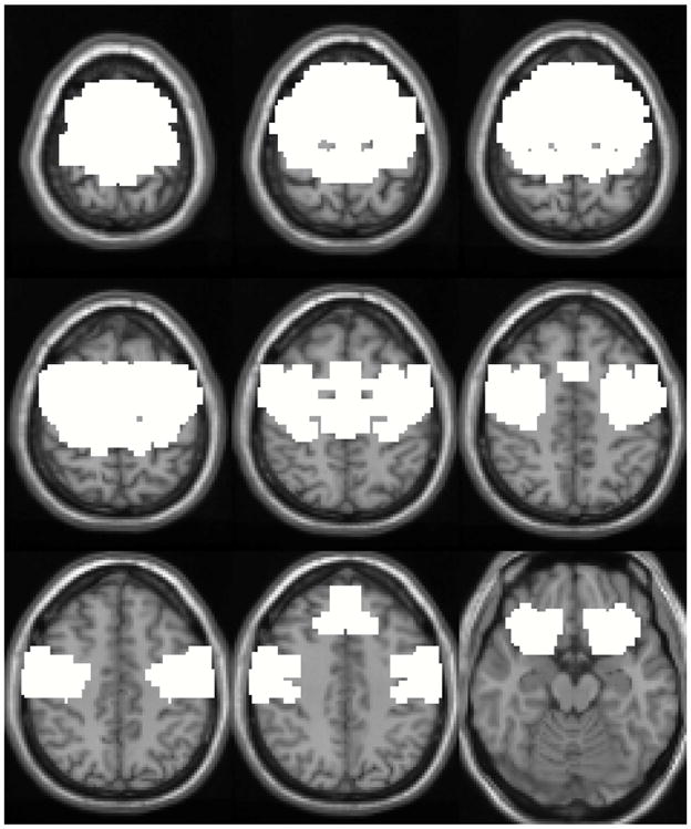
Binary mask identifying motor cortex area (Brodmann areas: 4, 6, 43 and 47).

We implemented parametric (Section 5.2.1) and non-parametric (Section 5.2.2) methods for thresholding the Z_c and Z_r sample values and calculated the receiver operating characteristic (ROC) curves for those. The probability of true positives (TP) in the generated ROC curves indicates the number of voxels that survive the threshold (at each point in the ROC curve) and that fall inside the motor cortex mask; similarly, the probability of false positive (FP) indicates the number of voxels that pass the various thresholds and that fall outside the motor cortex mask. Comparison of the ROC curves for the different thresholding methods is done by calculating the ratio of their respective area under the curve (AUC). The absolute value of the ROC curves area is not of interest since the test is not designed to obtain the typical ideal AUC value of 1.0. A AUC value of 1.0 is only obtained when all the voxels in the created motor cortex mask are identified at all the thresholds, which is impossible since by definition the ROC curves are created by gradually adding more voxels at each threshold. Better perfomance, as measured by the a higher AUC, indicates overall higher sensitivity and specificity at the various thresholds used in the ROC curves. Higher sensitivity means that a higher number of voxels are identified as active. Similarly, an increase in specificity indicates that a large number of the additional identified voxels are located inside the motor cortex area mask.

5.2.1. Parametric Results

In this section, the thresholds needed to create the ROC curves are obtained by approximating the distributions of the estimated average motor task-related independent component by various well known probability distribution functions (pdf). The Z_r values are usually approximated with a Gaussian pdf and probabilities calculated for each voxel, those with low probability in the tails of the distribution are assumed to be the active ones. Similarly, under the assumption that the real and imaginary data of the estimated ICs are bivariate Gaussian, the Z_c is approximated by a chi-square distribution with two degrees of freedom. The calculated probabilities for both Z_c and Z_r samples are used to threshold the estimated IC and create the ROC curves in Fig. 5 ( Z_c chi-square and Z_r Gaussian lines, respectively). The Z_c thresholding method provides better performance than the Z_r thresholding method as confirmed by the ratio of the AUC values: $\frac{\text{AUC}{Z}_r}{\text{AUC}{Z}_c}=0.77$ (see Table 1).

Figure 5.

ROC curves obtained for the Z_c, Z_r and magnitude data of the estimated average motor task-related IC under different assumed pdfs. Comparison of the ROC curves for the different thresholding methods is done by calculating the ratio of their respective area under the curve (AUC). The absolute value of the ROC curves area is not of interest since the test is not designed to obtain the typical ideal AUC value of 1.0.

Table 1.

Ratio of the AUC values of the ROC curves obtained from the Z_c, Z_r, magnitude and complex-valued data of the estimated average motor task-related under different assumed pdfs versus the AUC value of Z_c under the chi-square distribution: $\frac{\text{AUC}\text{method}}{\text{AUC}{Z}_c}$

Zc Chi2	Zr Gaussian	Bivariate Gaussian	Magnitude Chi2
1.0	0.77	1.0	0.95

Additional parametric thresholding methods were implemented to compare the performance of using the complex-valued data versus only using the magnitude of the IC data for visualization. The complex-valued data was thresholded by using a bivariate Gaussian distribution approximation for the real and imaginary data of the IC, the results was identical to the Z_c result (see Bivariate Gaussian result in Table 1). This identical result was expected since the two methods operate under the same assumption that the underlying real and imaginary data are bivariate Gaussian. The advantage of the Z_c method is that it contains the same information under a single positive number.

Various pdfs were used to approximate the distribution of the magnitude-only data of the estimated IC. The majority of the implemented distributions outperformed the Z_r results, but the best result was obtained by assuming that the real and imaginary data of the IC are independent standard Gaussian random variables, under this assumption the square magnitude has a chi-square distribution with two degrees of freedom(see Magnitude Chi² result in Table 1 and in Fig. 5). This result shows that by using a more appropriate approximation to the magnitude data better performance can be obtained.

A visual example of the increase in sensitivity and specificity obtained by using the Z_C thresholding method can be seen in Fig. 6. This figure shows the identified voxels with a probability of 0.01 calculated by the Z_c method under the chi-square distribution approximation and the Z_r method under the Gaussian distribution approximation. The voxels with a value of 2.0 were only identified by the Z_c method, and it can be seen that the majority of them are contiguous with the other identified motor task-related voxels by both the Z_c and Z_r methods. The majority of these additional detected voxels had low magnitude but significantly different phase values than the rest of the voxels.

Figure 6.

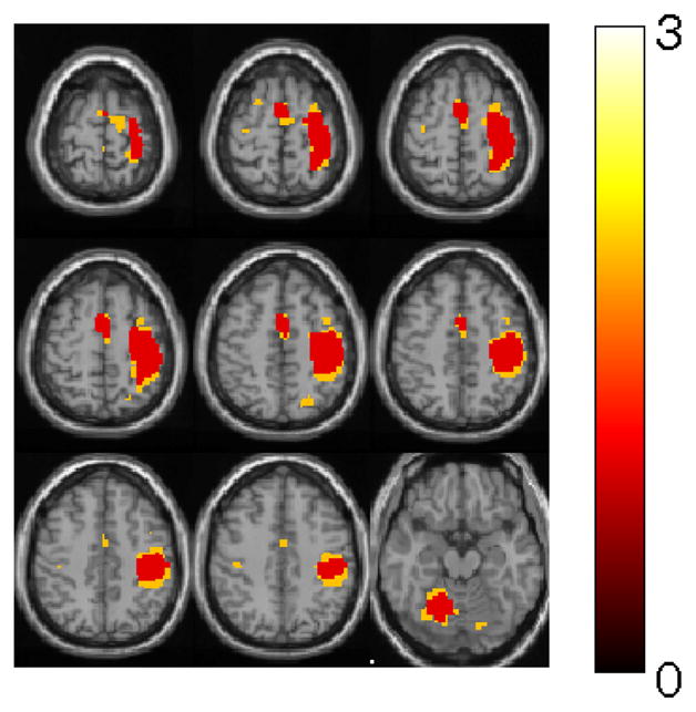
Identified voxels (with a probability of 0.01) by the Z_c method under the chi-square distribution approximation and the Z_r method under the Gaussian distribution approximation. Red voxels were identified by both methods. Yellow voxels are those that are identified only by Z_c.

The region detected by Z_c is typically larger than the one detected by Z_r, because as shown in [3] significant phase changes can be seen in regions where susceptibility (i.e. activation) is changing across a voxel. This typically happens in regions surrounding the center of activation, where activation is decreasing (as confirmed in Fig. 6).

The two main conclusions from this section are: (1) the two thresholding methods using the complex-valued data perform better and (2) there are better parametric approximations to threshold the magnitude-only data than the Z_r Gaussian distribution approximation.

5.2.2. Non-Parametric Results

Since parametric evaluations have to be based on an inherent assumption of sample distribution, we also used non-parametric methods to demonstrate that Z_c thresholding method provides better performance than the Z_r thresholding method. Fig. 7, shows the quantile-quantile (Q-Q) plot of the Z_r samples versus the Z_c sample values. The Q-Q plot is a graphical method for comparing two distributions by plotting their quantiles against each other [34], if the samples in a Q-Q plot come from the same distribution, the plot will be linear. The plot has the sample data displayed with the plot symbol (+), and superimposed on the plot is a line joining the first and third quartiles of each distribution (this is a robust linear fit of the order statistics of the two samples). This line is extrapolated out to the ends of the sample to help evaluate the linearity of the data ⁴. The Q-Q plot indicates that the Z_r samples have a more flat distribution than the Z_c samples as their values go up, this means that the Z_r samples are less discriminatory, which confirms our parametric results.

Figure 7.

QQ plot of Z_r values versus Z_c values. The Q-Q plot is a graphical method for comparing two distributions by plotting their quantiles against each other, if the samples in a Q-Q plot come from the same distribution, the plot will be linear.

Two new Z_r and Z_c ROC curves were created (see Fig. 8) by using the more classical definition of probability to identify active voxels. The same number (N) of the highest valued voxels are extracted from the Z_r and Z_c samples and used to calculate the different points of their respective ROC curves. The value of N for each point in the ROC curves is calculated by

Figure 8.

Non-parametric ROC curves obtained for the Z_c and Z_r samples. Comparison of the ROC curves is done by calculating the ratio of their respective area under the curve (AUC). The absolute value of the ROC curves area is not of interest since the test is not designed to obtain the typical ideal AUC value of 1.0.

$$N=(\text{Total}\text{voxels})P$$ (5)

where P takes values in [0, 1].

The AUC value for the non-parametric and parametric ROC curves of Z_c are identical. The AUC ratio between the non-parametric Z_r and Z_c ROC curves is 0.94. This ratio is has bigger value that the one calculated with the parametric Z_r result, but the conclusion is the same, using the entire complex-valued data increases the sensitivity and specificity in identifying activated voxels when compared to magnitude-only visualization. This increase in performance is obtained for free, since the data is inherently complex-valued.

5.3. ICA Phase Ambiguity Correction Results

5.3.1. ICA using Non-linear Decorrelations with atanh Non-linearity

We applied complex-valued ICA using atanh as the non-linearity as described in section 3.1, hence no phase ambiguity correction is needed for the estimates, except for maybe a sign correction. Fig. 10, shows the magnitude, phase and Z_c image—of selected slices—for a motor task related component identified and averaged across all the subjects. The average is performed on the magnitude and phase domain, but similar results were obtained when calculating the average in the real and imaginary domains. The motor component is identified automatically by regressing the estimated time-courses with the ideal hemodynamic time response. The results obtained here show that it is possible to obtain clear magnitude and phase images of components of interest in group studies. The obtained group phase images have the expected bipolar distributions, smoothness, continuity and characteristics as described in [3]. In the next section we show how the phase images of different subjects with no phase ambiguity correction can add destructively, hence creating group images with lower magnitude and noisy phase images.

Figure 10.

Average magnitude, phase and Z_c maps for the estimated motor component using atanh non-linearity. Voxels with a |Z_c| > 3.5 and good quality were identified as voxels of interest.

5.3.2. ICA using Infomax with a Circular Non-linearity

Next, we estimate spatial independent components from the group fMRI data using the Infomax algorithm [23] with the circular nonlinear function proposed in [35], which does not impose any particular orientation to the distribution of the estimated sources. The obtained group ICA results at this point can be used to identify the motor task component only in the magnitude image. Applying the post-ICA phase ambiguity correction scheme described in section 3.2 to the estimated components in each subject makes group analysis of the entire complex-valued images possible by eliminating the phase ambiguity across subjects. Fig. 11 shows the scatter plot of the average real and imaginary values of the identified motor component in our fMRI group data after phase ambiguity correction. Additionally, Fig. 12 shows the corresponding magnitude, phase and Z_c images for the estimated component. It can be clearly seen that the identified motor task-related voxels correlate with the identified voxels in Fig. 10, where our post-processing phase ambiguity correction was not necessary.

Figure 11.

The average real and imaginary values of the fMRI group estimated motor component after phase ambiguity correction.

Figure 12.

Average magnitude, phase and Z_c maps for the estimated group motor component using Infomax algorithm with circular non-linearity after phase ambiguity correction. Voxels with a |Z_c| > 4.0 and good quality were identified as voxels of interest.

To emphasize the importance of the phase ambiguity correction step, we present the ICA results obtained from the fMRI group data prior to applying the post-processing phase ambiguity correction. In Fig. 13, we can see the scatter plot of the group average real and imaginary values of the identified motor component before phase ambiguity correction. The voxels of the estimated motor component of each subject (including subject one in Fig. 2.a) add destructively, hence creating a more spread scatter plot of voxels with lower magnitude and less smooth phase values when compared to the results in Fig. 11. Fig. 14 shows the magnitude, Z_c and phase of the estimated component prior to phase ambiguity correction, although we can still identify task related voxels, they are not as discriminatory, i.e., lower number of identified voxels with lower magnitude values in the motor cortex brain areas of interest. Additionally, in the phase image we can see that the phase changes across voxels are indeed not as smooth and continuous, as the results obtained with phase ambiguity correction.

Figure 13.

The average real and imaginary values of the fMRI group estimated motor component, but with no post-processing phase ambiguity correction.

Figure 14.

Average magnitude, phase and Z_c maps for the estimated group motor component using Infomax algorithm with circular non-linearity but with no post-processing phase ambiguity correction. Voxels with a |Z_c| > 4.0 and good quality were identified as voxels of interest.

In Fig. 9, the ROC curves obtained for Z_c with and without phase ambiguity correction are shown. The calculated ROC curves used the same motor cortex mask and the same non-parametric technique used in Section 5.2.2. It can be seen that the AUC of Z_c without phase ambiguity correction is lower than the AUC of Z_c with phase ambiguity correction, their ratio is equal to 0.93. Additionally, the results of Z_c without phase ambiguity correction were found to be almost identical to the results obtained with Z_r thresholding method, this corroborates the finding in [Rowe and Logan NIMG 2005] that processing complex-valued fMRI data assuming non-informative phase information is identical to magnitude-only processing.

Figure 9.

Non-parametric ROC curves obtained for Z_r and for Z_c, with and without phase ambiguity correction. Comparison of the ROC curves for the different thresholding methods is done by calculating the ratio of their respective area under the curve (AUC). The absolute value of the ROC curves area is not of interest since the test is not designed to obtain the typical ideal AUC value of 1.0.

Similar results are obtained with the estimated timecourses (i.e., mixing matrix) when the phase ambiguity correction is applied. In Fig. 15, we show the average group magnitude and phase timecourses for the motor task IC prior and after phase ambiguity correction. As expected, the magnitude and phase of the timecourses after phase ambiguity correction have a stronger correlation with the paradigm timecourse convolved with the hemodynamic response (see correlation coefficient values for each timecourse in Fig. 15). The average timecourse calculations were performed in the real and imaginary domain, but similar benefits were obtained when calculating the average in the magnitude and phase domain, particularly for the phase.

Figure 15.

Average magnitude and phase timecourses for the estimated motor component using Infomax algorithm with circular non-linearity prior (a,b) and after (c,d) phase ambiguity correction. The correlation coefficient (ρ) between each of the displayed magnitude and phase timecourses and the paradigm timecourse convolved with the hemodynamic response are shown below the respective figures.

6. DISCUSSION

Robust techniques that can show the advantages of using the phase information in the identification and analysis of voxels of interest in complex-valued fMRI data are needed. Even in applications where complex-valued algorithms are used to analyze the fMRI data, the majority of the preprocessing and visualization methods used are based on the magnitude images. The phase images are usually discarded, primarily because their unfamiliar and noisy nature poses a challenge for successful study of fMRI We addressed some of these issues and proposed methods that allow the successful analysis of complex-valued fMRI group data. This could strengthen the traditional analysis methods as well as those of data-driven techniques such as ICA by improving their performance in identifying voxels of interest.

We introduced two effective schemes that can be used to diminish the inherent phase scaling ambiguity of complex-valued ICA to allow for group analysis. The phase ambiguity correction scheme can be either applied subsequent to ICA of fMRI or can be incorporated into the ICA algorithm in the form of prior information—when available—to eliminate the need for further processing. Additionally, we presented a Mahalanobis distance-based visualization method that uses the phase in the estimated fMRI sources to identify task—functional—related voxels. We were able to show that these methods provide better sensitivity and specifity, than magnitude-only visualization methods, when identifying voxels in a estimated motor task-related independent component. This method shows particular promise for identifying voxels with significant susceptibility changes but that are located in low magnitude areas as modeled in [3].

The introduced methods are part of a framework that allows the utilization of the phase in the analysis of complex fMRI data, in particular using ICA that has already shown to hold much promise for the task. Future work will concentrate on using the results of our complex-valued analysis of the fMRI data to see if we can enhance the performance of classification algorithms in clinical studies.

References

- 1.Kwong K, et al. Dynamic magnetic resonance imaging of human brain activity during primary sensory stimulation. Proc Natl Acad Sci. 1992;89:5675–5679. doi: 10.1073/pnas.89.12.5675. [DOI] [PMC free article] [PubMed] [Google Scholar]
- 2.Calhoun VD, Adalı T, Pearlson GD, van Zijl PCM, Pekar JJ. Independent component analysis of fMRI data in the complex domain. Magnetic Resonance in Medicine. 2002;48:180–192. doi: 10.1002/mrm.10202. [DOI] [PubMed] [Google Scholar]
- 3.Feng Z, Caprihan A, Blagoev KB, Calhoun VD. Biophysical modeling of phase changes in Bold fMRI. NeuroImage. 2010 doi: 10.1016/j.neuroimage.2009.04.076. In Press. [DOI] [PMC free article] [PubMed] [Google Scholar]
- 4.Rowe DB. Modeling both the magnitude and phase of complex-valued fMRI data. NeuroImage. 2005;25:1310–1324. doi: 10.1016/j.neuroimage.2005.01.034. [DOI] [PubMed] [Google Scholar]
- 5.Hoogenrad F, Reichenbach J, Haacke E, Lai S, Kuppusamy K, Sprenger M. In vivo measurement of changes in venous blood-oxygenation with high resolution functional mri at .95 tesla by measuring changes in susceptibility and velocity. Magn Reson Med. 1998;39:97–107. doi: 10.1002/mrm.1910390116. [DOI] [PubMed] [Google Scholar]
- 6.Arja S, Feng Z, Chen Z, Caprihan A, Kiehl K, Adalı T, Calhoun V. Changes in fMRI magnitude data and phase data observed in block-design and event-related tasks. NeuroImage. 2010 doi: 10.1016/j.neuroimage.2009.10.087. In Press. [DOI] [PMC free article] [PubMed] [Google Scholar]
- 7.Chen Z, Caprihan A, Calhoun V. Effect of surrounding vasculature on intravoxel bold signal. Med Phys. 2010;37:1778–1787. doi: 10.1118/1.3366251. [DOI] [PMC free article] [PubMed] [Google Scholar]
- 8.Menon R. Postacquisition suppression of large-vessel bold signals in high-resolution fmri. Magn Reson Med. 2002;47:1–9. doi: 10.1002/mrm.10041. [DOI] [PubMed] [Google Scholar]
- 9.Xiong W, Li YO, Li H, Adalı T. On ICA of complex-valued fMRI: Advantages and order selection. Proc. IEEE Int. Conf. Acoust., Speech, Signal Processing (ICASSP); Las Vegas, Nevada. 2008. [Google Scholar]
- 10.Li H, Adalı T, Correa N, Rodriguez P, Calhoun V. Flexible complex ICA of FMRI data. Proc. IEEE Int. Conf. Acoust., Speech, Signal Processing (ICASSP); 2010. [Google Scholar]
- 11.Calhoun VD, Adalı T, Li YO. Independent component analysis of complex-valued functional MRI data by complex nonlinearities. Proc. IEEE Int. Symp. Bio. Imag. (ISBI); Arlington, VA. 2004. [Google Scholar]
- 12.Rodriguez P, Adalı T, Li H, Correa N, Calhoun V. Phase correction and denoising for ICA of complex FMRI data, submitted to IEEE Int. Conf. Acoust., Speech, Signal Processing (ICASSP); 2010. [Google Scholar]
- 13.Rodriguez P, Correa N, Adalı T, Calhoun V. Quality map thresholding for de-noising of complex-valued fMRI data and its application to ICA of fMRI. Proc. IEEE Machine Learning for Signal Processing (MLSP); 2009. [DOI] [PMC free article] [PubMed] [Google Scholar]
- 14.Rodriguez P, Correa N, Eichele T, Calhoun V, Adalı T. Quality map thresholding for de-noising of complex-valued fMRI data and its application to ICA of fMRI. Journal of Signal Processing Systems. 2010 doi: 10.1007/s11265-010-0536-z. [DOI] [PMC free article] [PubMed] [Google Scholar]
- 15.Bell A, Sejnowski T. An information maximization approach to blind separation and blind deconvolution. Neural Computation. 1995;7:1129–1159. doi: 10.1162/neco.1995.7.6.1129. [DOI] [PubMed] [Google Scholar]
- 16.Hyvarinen A, Karhunen J, Oja E. Independent Component Analysis. John Wiley and Sons Inc; New York, USA: 2001. [Google Scholar]
- 17.Comon P. Independent component analysis: A new concept? Signal Processing. 1994;36:11–20. [Google Scholar]
- 18.McKeown MJ, et al. Spatially independent activity patterns in functional magnetic resonance imaging data during the stroop color-naming task. Proc Natl Acad Sci USA. 1998;95:803–810. doi: 10.1073/pnas.95.3.803. [DOI] [PMC free article] [PubMed] [Google Scholar]
- 19.McKeown MJ, et al. Analysis of fMRI data by blind separation into independent spatial components. Human Brain Mapping. 1998;6:160–188. doi: 10.1002/(SICI)1097-0193(1998)6:3<160::AID-HBM5>3.0.CO;2-1. [DOI] [PMC free article] [PubMed] [Google Scholar]
- 20.Calhoun VD, Adalı T. Unmixing fMRI with independent component analysis. IEEE Eng Med Bio Mag. 2006;25:79–90. doi: 10.1109/memb.2006.1607672. [DOI] [PubMed] [Google Scholar]
- 21.Calhoun V, Liu J, Adalı T. A review of group ICA for fMRI data and ICA for joint inference of imaging, genetic, and erp data. Neuroimage. 2009;45:163–172. doi: 10.1016/j.neuroimage.2008.10.057. [DOI] [PMC free article] [PubMed] [Google Scholar]
- 22.Li YO, Adalı T, Calhoun VD. Estimating the number of independent components for fMRI data. Hum Brain Mapping. 2007;28:1251–1266. doi: 10.1002/hbm.20359. [DOI] [PMC free article] [PubMed] [Google Scholar]
- 23.Adalı T, Kim T, Calhoun VD. Independent component analysis by complex nonlinearities. Proc. IEEE Int. Conf. Acoust., Speech, Signal Processing (ICASSP); Montreal, Canada. 2004. pp. 525–528. [Google Scholar]
- 24.Novey M, Adalı T. Complex ICA by negentropy maximization. IEEE Trans Neural Networks. 2008;19:596–609. doi: 10.1109/TNN.2007.911747. [DOI] [PubMed] [Google Scholar]
- 25.Li XL, Adalı T. Complex independent component analysis by entropy bound minimization; IEEE Trans Circuits and Systems I; 2010. In Press. [Google Scholar]
- 26.Adalı T, Li H. A practical formulation for computation of complex gradients and its application to maximum likelihood. Proc. IEEE Int. Conf. Acoust., Speech, Signal Processing (ICASSP); 2007. [Google Scholar]
- 27.Gazzah H, Regalia P, Delmas J, Calhoun V, Abed-Meraim K. A blind multichannel identification algorithm robust to order overestimation. IEEE Trans Signal Processing. 2010;50:1449–1558. [Google Scholar]
- 28.Hardy E, Hoferer J, Mertens D, Kasper G. Automated phase correction via maximization of the real signal. Magnetic Resonance Imaging (MRI) 2009;27:393–400. doi: 10.1016/j.mri.2008.07.009. [DOI] [PubMed] [Google Scholar]
- 29.Noll D, Nishimura D, Macovski A. Homodyne detection in magnetic resonance imaging. IEEE Trans Med Imaging. 1991;10:154–163. doi: 10.1109/42.79473. [DOI] [PubMed] [Google Scholar]
- 30.Bernstein M, Thomasson D, Perman W. Improved detectability in low signal-to-noise ratio magnetic resonance images by means of a phase-corrected real reconstruction. Med Phys. 1989;16:813–817. doi: 10.1118/1.596304. [DOI] [PubMed] [Google Scholar]
- 31.Adalı T, Li H. A practical formulation for computation of complex gradients and its application to maximum likelihood ICA. Proc. IEEE Int. Conf. Acoust., Speech, Signal Processing (ICASSP); Honolulu, Hawaii. 2007. pp. II–613–II–636. [Google Scholar]
- 32.Cardoso JF, Souloumiac A. Blind beamforming for non-Gaussian signals. IEEE Proc Radar Signal Processing. 1993;140:362–370. [Google Scholar]
- 33.Ghiglia DC, Pritt MD. Two-Dimensional Phase Unwrapping. Wiley; New York, USA: 1998. [Google Scholar]
- 34.Gnanadesikan R, Wilk M. Probability plotting methods for the analysis of data. Biometrika. 1968;55:1–17. [PubMed] [Google Scholar]
- 35.Anemüller J, Sejnowski TJ, Makeig S. Complex independent component analysis of frequency-domain electroencephalographic data. Neural Networks. 2003;16:1311–1323. doi: 10.1016/j.neunet.2003.08.003. [DOI] [PMC free article] [PubMed] [Google Scholar]