Causality Analysis of Neural Connectivity: Critical Examination of Existing Methods and Advances of New Methods

Abstract

Granger causality (GC) is one of the most popular measures to reveal causality influence of time series and has been widely applied in economics and neuroscience. Especially, its counterpart in frequency domain, spectral GC, as well as other Granger-like causality measures have recently been applied to study causal interactions between brain areas in different frequency ranges during cognitive and perceptual tasks. In this paper, we show that: 1) GC in time domain cannot correctly determine how strongly one time series influences the other when there is directional causality between two time series, and 2) spectral GC and other Granger-like causality measures have inherent shortcomings and/or limitations because of the use of the transfer function (or its inverse matrix) and partial information of the linear regression model. On the other hand, we propose two novel causality measures (in time and frequency domains) for the linear regression model, called new causality and new spectral causality, respectively, which are more reasonable and understandable than GC or Granger-like measures. Especially, from one simple example, we point out that, in time domain, both new causality and GC adopt the concept of proportion, but they are defined on two different equations where one equation (for GC) is only part of the other (for new causality), thus the new causality is a natural extension of GC and has a sound conceptual/theoretical basis, and GC is not the desired causal influence at all. By several examples, we confirm that new causality measures have distinct advantages over GC or Granger-like measures. Finally, we conduct event-related potential causality analysis for a subject with intracranial depth electrodes undergoing evaluation for epilepsy surgery, and show that, in the frequency domain, all measures reveal significant directional event-related causality, but the result from new spectral causality is consistent with event-related time–frequency power spectrum activity. The spectral GC as well as other Granger-like measures are shown to generate misleading results. The proposed new causality measures may have wide potential applications in economics and neuroscience.

I. Introduction

GIVEN a set of time series, how to define causality influence among them has been a topic for over 2000 years and is yet to be completely resolved [1]–[3]. In the literature, one of the most popular definitions for causality is Granger causality (GC). Due to its simplicity and easy implementation, GC has been widely used. The basic idea of GC was originally conceived by Wiener [4] and later formalized by Granger in the form of linear regression model [5]. It can be simply stated as follows. If the variance $\left({\sigma }_{{∊}_1}^2\right)$ of the prediction error for the first time series at the present time is greater than the variance $\left({\sigma }_{{\eta }_1}^2\right)$ of the prediction error by including past measurements from the second time series in the linear regression model, then the second time series can be said to have a causal (driving) influence on the first time series. Reversing the roles of the two time series, one repeats the process to address the question of driving in the opposite direction. GC value of $\ln ({\sigma }_{{∊}_1}^2∕{\sigma }_{{\eta }_1}^2)$ is defined to describe the strength of the causality that the second time series has on the first one [5]–[10]. From GC value, it is clear that: 1) $\ln ({\sigma }_{{∊}_1}^2∕{\sigma }_{{\eta }_1}^2)=0$ when there is no causal influence from the second time series to the first one and $\ln ({\sigma }_{{∊}_1}^2∕{\sigma }_{{\eta }_1}^2)>0$ when there is, and 2) the larger the value of $\ln ({\sigma }_{{∊}_1}^2∕{\sigma }_{{\eta }_1}^2)$, the higher causal influence. In recent years, there has been significant interest to discuss causal interactions between brain areas which are highly complex neural networks. For instance, with GC analysis Freiwald et al. [7] revealed the existence of both unidirectional and bidirectional influences between neural groups in the macaque inferotemporal cortex. Hesse et al. [9] analyzed the electroencephalogram (EEG) data from the Stroop task and disclosed that conflict situations generate dense webs of interactions directed from posterior to anterior cortical sites and the web of directed interactions occurs mainly 400 ms after the stimulus onset and lasts up to the end of the task. Roebroeck et al. [11] explored directed causal influences between neuronal populations in functional magnetic resonance imaging (fMRI) data. Oya et al. [10] demonstrated causal interactions between auditory cortical fields in humans through intracranial evoked potentials to sound. Gow et al. [12] applied Granger analysis to MRI-constrained magnetoencephalogram and EEG data to explore the influence of lexical representation on the perception of ambiguous speech sounds. Gow et al. [13] showed a consistent pattern of direct posterior superior temporal gyrus influence over sites distributed over the entire ventral pathway for words, non-words, and phonetically ambiguous items.

Since frequency decompositions are often of particular interest for neurophysiological data, the original GC in time domain has been extended to spectral domain. Along this line, several spectral Granger or Granger-like causality measures have been developed such as spectral GC [6], [8], conditional spectral GC [6], [8], partial directed coherence (PDC) [14], relative power contribution (RPC) [15], directed transfer function (DTF) [16], and short-time direct directed transfer function (SdDTF) [17]. For two time series, spectral GC, PDC, RPC, and DTF are all equivalent in the sense that, when one of them is zero, the others are also zero. The applications of these measures to neural data have yielded many promising results. For example, Bernasconi and Konig [18] applied Geweke's spectral measures to describe causal interactions among different areas in the cat visual cortex. Liang et al. [19] used a time-varying spectral technique to differentiate feedforward, feedback, and lateral dynamical influences in monkey ventral visual cortex during pattern discrimination. Brovelli et al. [20] applied spectral GC to identify causal influences from primary somatosensory cortex to motor cortex in the beta band (15–30 Hz) frequency during lever pressing by awake monkeys. Ding et al. [6] discussed conditional spectral GC to reveal that causal influence from area S1 to interior posterior parietal area 7a was mediated by the inferior posterior parietal area 7b during monkey visual pattern discrimination task. Sato et al. [21] applied PDC to fMRI to discriminate physiological and nonphysiological components based on their frequency characteristics. Yamashita et al. [15] applied RPC to evaluate frequency-wise directed connectivity of BOLD signals. Kaminski and Liang [22] applied short-time DTF to show predominant direction of influence from hippocampus to supramammilary nucleus at the theta band (3.7–5.6 Hz) frequency. Korzeniewska et al. [17] used SdDTF to reveal frequency-dependent interactions, particularly in high gamma (> 60 Hz) frequencies, between brain regions known to participate in the recorded language task.

In time domain, the well-known GC value defined by $\ln ({\sigma }_{{∊}_1}^2∕{\sigma }_{{\eta }_1}^2)$ is only related to noise terms of the linear regression models and has nothing to do with coefficients of the linear regression model of two time series. As a result, this definition may miss some important information and may not be able to correctly reflect the real strength of causality when there is directional causality from one time series to the other. That is, the larger GC value does not necessarily mean higher causality, or vice versa, although in general this definition is very useful to determine whether there is directional causality between two time series, that is, $\ln ({\sigma }_{{∊}_1}^2∕{\sigma }_{{\eta }_1}^2)=0$ means no causality and $\ln ({\sigma }_{{∊}_1}^2∕{\sigma }_{{\eta }_1}^2)\ne 0$ means existence of causality. Therefore, the GC value may not correctly reflect real causal influence between two channels. In other words, GC values for different pairs of channels even from the same subject may not be comparable. As such, the common practice of using thickness of arrows in a diagram to represent the strength of causality for different pairs of channels even in the same subject may not be true. In the literature, the other GC value defined in [7] is only related to one column of the coefficient matrix of the linear regression model and has nothing to do with the terms in other columns and noise terms. This also makes this definition suffer from similar pitfalls. Therefore, a researcher must use caution when drawing any conclusion based on these two GC values. In the frequency domain, the spectral GC is defined by Granger [5] based on the inverse matrix of the transfer matrix and the noise terms of the linear regression model and called it causality coherence. This definition in nature is a generalization of coherence where researchers have already realized that coherence cannot be used to reveal real causality for two time series. For this reason, since then various definitions of GC in frequency domain have been developed. Among the most popular definitions are the spectral GC [6] and [8], PDC [14], RPC [15], and DTF [16]. The spectral GC can be applied to two time series or two groups of time series, PDC, RPC, and DTF can be applied to multidimensional time series. DTF and RPC are not able to distinguish between direct and indirect pathways linking different structures and as a result they do not provide the multivariate relationships from a partial perspective [21]. PDC lacks a theoretical foundation [23]. In general, the above spectral Granger or Granger-like causality definitions are based on the transfer function matrix (or its inverse matrix) of the linear regression model and thus may not be able to reflect the real strength of causality as pointed out later in detail in this paper. Note that the transfer function matrix or its inverse matrix is different from the coefficient matrix of the linear regression model (frequency model), on which we rely in this paper to propose new spectral causality.

In this paper, on one hand, in time domain we define a new causality from any time series Y to any time series X in the linear regression model of multivariate time series, which describes the proportion that Y occupies among all contributions to X. Especially, we use one simple example to show that both the new causality and GC adopt the concept of proportion, but they are defined on two different equations where one equation (for GC) is only part of the other equation (for new causality), and therefore the new causality is a natural extension of GC and GC is not the desired causal influence at all. As such, even when the GC value is zero, there still exists a real causality which can be revealed by a new causality. Therefore, the popular traditional GC cannot reveal the real strength of causality at all and researchers must apply caution in drawing any conclusion based on the GC value. On the other hand, in frequency domain we point out that any causality definition based on the transfer function matrix (or its inverse matrix) of the linear regression model in general may not be able to reveal the real strength of causality between two time series. Since almost all existing spectral causality definitions are based on the transfer function matrix (or its inverse matrix) of the linear regression model, we take the widely used spectral GC, PDC, and RPC as examples and point out their inherent shortcomings and/or limitations. To overcome these difficulties, we define a new spectral causality that describes the proportion that one variable occupies among all contributions to another variable in the multivariate linear regression model (frequency domain). By several simulated examples, one can clearly see that our new definitions (in time and frequency domain) are advantageous over existing definitions. In particular, for a real event-related potential (ERP) EEG data from a seizure patient, the application of new spectral causality shows promising and reasonable results. But the applications of spectral GC, PDC, and RPC all generate misleading results. Therefore, our new causality definitions may open a new window to study causality relationships and may have wide applications in economics and neuroscience.

This paper is organized as follows. Causality analyses in time domain and frequency domain are discussed in Section II and Section III, respectively. Several examples are provided in Section IV. Concluding remarks are given in Section V.

II. Granger Causality in Time Domain

In this section, we first introduce the well-known GC and conditional GC, and then we define a new causality.

We begin with a bivariate time series. Given two time series X₁(t) and X₂(t). which are assumed to be jointly stationary, their autoregressive representations are described as

$$\{\begin{array}{c}{X}_{1,t}=\sum _{j=1}^m{\mathbf{a}}_{11,j}{X}_{1,t-j}+{∊}_{1,t}\hfill \\ X_{2,t}=\sum _{j=1}^m{\mathbf{a}}_{22,j}{X}_{2,t-j}+{∊}_{2,t}\hfill \end{array}\phantom{\}}$$ (1)

and their joint representations are described as

$$\{\begin{array}{c}{X}_{1,t}=\sum _{j=1}^m{a}_{11,j}{X}_{1,t-j}+\sum _{j=1}^m{a}_{12,j}{X}_{2,t-j}+{\eta }_{1,t}\hfill \\ X_{2,t}=\sum _{j=1}^m{a}_{21,j}{X}_{1,t-j}+\sum _{j=1}^m{a}_{22,j}{X}_{2,t-j}+{\eta }_{2,t}\hfill \end{array}\phantom{\}}$$ (2)

where t = 0, 1, . . . , N, the noise terms are uncorrelated over time, ε_i and η_i have zero means and variances of ${\sigma }_{{∊}_i}^2$, and ${\sigma }_{{\eta }_i}^2$, i = 1, 2. The covariance between η₁ and η₂ is defined by σ_η1η2 = cov(η₁, η₂).

Now consider the first equalities in (1) and (2). According to the original formulations in [4] and [5], if ${\sigma }_{{\eta }_1}^2$ is less than ${\sigma }_{{∊}_1}^2$ in some suitable statistical sense, X₂ is said to have a causal influence on X₁. In this case, the first equality in (2) is more accurate than that in (1) to estimate X₁. Otherwise, if ${\sigma }_{{\eta }_1}^2={\sigma }_{{∊}_1}^2$, X₂ is said to have no causal influence on X₁. In this case, two equalities are same. Such kind of causal influence, called GC [6], [8], is defined by

$$F_{X_2\to X_1}=\ln \frac{{\sigma }_{{∊}_1}^2}{{\sigma }_{{\eta }_1}^2}.$$ (3)

Obviously, F_X2→X1 = 0 when there is no causal influence from X₂ to X₁ and F_X2→X1 > 0 when there is. Similarly, the causal influence from X₁ to X₂ is defined by

$$F_{X_1\to X_2}=\ln \frac{{\sigma }_{{∊}_2}^2}{{\sigma }_{{\eta }_2}^2}.$$ (4)

To show whether the interaction between two time series is direct or is mediated by another recorded time series, conditional GC [6], [24] was defined by

$$F_{X_2\to X_1\mid X_3}=\ln \frac{{\sigma }_{{∊}_3}^2}{{\sigma }_{{\eta }_3}^2}$$ (5)

where ${\sigma }_{{∊}_3}^2$ and ${\sigma }_{{\eta }_3}^2$ are the variances of two noise terms ε₃ and η₃ of the following two joint autoregressive representations:

$$X_{1,t}=\sum _{j=1}^m{\mathbf{a}}_{11,j}{X}_{1,t-j}+\sum _{j=1}^m{\mathbf{a}}_{13,j}{X}_{3,t-j}+{∊}_{3,t}$$ (6)

and

$$X_{1,t}=\sum _{j=1}^m{a}_{11,j}{X}_{1,t-j}+\sum _{j=1}^m{a}_{12,j}{X}_{2,t-j}+\sum _{j=1}^m{a}_{13,j}{X}_{3,t-j}+{\eta }_{3,t}.$$ (7)

According to this definition, F_X2→X1|X3 = 0 means that no further improvement in the prediction of X₁ can be expected by including past measurements of X₂. On the other hand, when there is still a direct component from X₂ to X₁, the past measurements of X₁, X₂, and X₃ together result in better prediction of X₁, leading to ${\sigma }_{{\eta }_3}^2<{\sigma }_{{∊}_3}^2$, and F_X2→X1|X3 > 0.

For GC, we point out some properties as follows.

Property 1:

1. Consider the following model:

   $$\{\begin{array}{c}{X}_{1,t}=a_{12,1}{X}_{2,t-1}+{\eta }_{1,t}\hfill \\ X_{2,t}=0.8X_{2,t-1}+{\eta }_{2,t}\hfill \end{array}\phantom{\}}$$ (8)

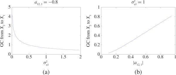
   where η₁, η₂ are two independent white noise processes with zero mean and variances ${\sigma }_{{\eta }_2}^2=1$ Fig. 1 shows GC values in two cases: a) a_{12, 1} = –0.8 and ${\sigma }_{{\eta }_1}^2$ varies from 0.01 to 2; b) a_{12, 1} varies from –0.1 to –0.95 and ${\sigma }_{{\eta }_1}^2=1$. From Fig. 1(a) and (b), one can see that the GC value from X₂ to X₁ decreases as the variance ${\sigma }_{{\eta }_1}^2$ increases (or increases as the amplitude |a_{12, 1}| increases). That means that increasing the amplitude |a_{12, 1}| or decreasing variance of the residual term η₁ will increase the GC value from X₂ to X₁. Thus, we conclude that GC is actually a relative concept, a larger GC value from X₂ to X₁ means that the causal influence from the first term a_{12, 1}X_2,t– occupies a larger portion compared to the influence from the residual term η_{1, t}, or vice versa.
2. Consider the following model:

   $$\{\begin{array}{c}{X}_{1,t}=a_{11,1}{X}_{1,t-1}-0.8X_{2,t-1}+{\eta }_{1,t}\hfill \\ X_{2,t}=a_{21,1}{X}_{1,t-1}+0.8X_{2,t-1}+{\eta }_{2,t}\hfill \end{array}\phantom{\}}$$ (9)

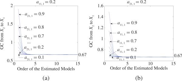
   where 0 < a_{11 , 1}, a_{21, 1} < 1 and for simplicity η₁, η₂ are assumed to be two independent white-noise processes with zero mean and variances ${\sigma }_{{\eta }_1}^2=1={\sigma }_{{\eta }_2}^2$. Fig. 2 shows GC from X₂ to X₁ for (9) under different parameters a_{11, 1} and a_{21, 1}. When we calculate GC, it should be pointed out that for each specific (9) we generate a dataset of 200 realizations of 10 000 time points. For each realization, we estimate AR models [autoregressive representations (1) and joint representations (2)] with the order of 8 by using the least-squares method and calculate GC where the order 8 fits well for all examples throughout this paper [see Fig. 2(a) and (b) from which one can see GC keeps steady when the order of the estimated models is greater than 8]. Then we obtain the average value across all realizations and get GC from X₂ to X₁. From Fig. 2, one can clearly see that GC from X₂ to X₁ has nothing to do with parameters a_{11, 1} and a_{21, 1} [of course, choices of parameters a_{11, 1} and a_{21, 1} are such that (9) does not diverge]. This property is consistent with the spectral GC result introduced later.

3. For (2), if η_2,t ≡ 0 or η_{1, t} = η_{2, t}, GC from X₂ to X₁ equals zero. This can be proved from (17.29), [6] and the spectral GC (32) introduced later.

Fig. 1.

(a) GC values from X₂ to X₁ in (8) as the variance ${\sigma }_{{\eta }_1}^2$ changes from 0.01 to 2 where a_{12, 1} = –0.8. (b) GC values from X₂ to X₁ in (8) as a_{12, 1} changes from –0.1 to –0.95 where ${\sigma }_{{\eta }_1}^2=1$. From (a) one can see that GC value from X₂ to X₁ decreases as the variance ${\sigma }_{{\eta }_1}^2$ increases. From (b) one can see that GC value from X₂ to X₁ increases as the amplitude |a_{12, 1}| increases.

Fig. 2.

(a) GC from X₂ to X₁ as a function of the order of the estimated models for (9) when a_{11, 1} = 0.2 and a_{21, 1} changes from 0.1 to 0.9. (b) GC from X₂ to X₁ as a function of the order of the estimated models for (9) when a_{21, 1} = 0.2 and a_{11, 1} changes from 0.1 to 0.9. From (a) and (b), one can see that: 1) GC from X₂ to X₁ keeps steady and converges to 0.67 when the order p > 8, and 2) GC from X₂ to X₁ has nothing to do with parameters a_{11, 1} and a_{21, 1}.

Except for the two specific cases in (iii) of Property 1, in general GC and conditional GC are useful to show whether theoretically there is directional interaction between two neurons or among three neurons. When there exists causal influence, a question arises: does the GC value or the conditional GC value reveal the real strength of causality? to answer this question, let us consider the following simple model:

$$\{\begin{array}{c}{X}_{1,t}=a_{12,1}{X}_{2,t-1}+{\eta }_{1,t}\hfill \\ X_{2,t}=a_{21,1}{X}_{1,t-1}+{\eta }_{2,t}\hfill \end{array}\phantom{\}}$$ (10)

where η₁ and η₂ are two independent white-noise processes with zero mean and a_{12, 1}a_{21, 1} ≠ 0. From (10), one can get

$$\begin{array}{cc}\hfill X_{1,t}& =a_{12,1}\left(\stackrel{X_{2,t-1}}{\overbrace{a_{21,1}{X}_{1,t-2}+{\eta }_{2,t-1}}}\right)+{\eta }_{1,t}\hfill \\ \hfill & =a_{12,1}{a}_{21,1}{X}_{1,t-2}+a_{12,1}{\eta }_{2,t-1}+{\eta }_{1,t}.\hfill \end{array}$$ (11)

So, the GC value

$$F_{X_2\to X_1}=\ln \frac{a_{12,1}^2{\sigma }_{{\eta }_2}^2+{\sigma }_{{\eta }_1}^2}{{\sigma }_{{\eta }_1}^2}=-\ln \left(1-\frac{a_{12,1}^2{\sigma }_{{\eta }_2}^2}{a_{12,1}^2{\sigma }_{{\eta }_2}^2+{\sigma }_{{\eta }_1}^2}\right)\in [0,+\infty )$$ (12)

or equivalently

$$F_{X_2\to X_1}=\frac{a_{12,1}^2{\sigma }_{{\eta }_2}^2}{a_{12,1}^2{\sigma }_{{\eta }_2}^2+{\sigma }_{{\eta }_1}^2}\in [0,1]$$ (13)

which is only related to the last two noise terms and has nothing to do with the first term. It is noted that all three terms make contributions to current X_1,t, and a_{12, 1}a_{21, 1}X₁, t–2 must have causal influence on X_{1, t} and must be considered to illustrate real causality. Especially, when ${\sigma }_{{\eta }_2}^2=0$, we have X_{1, t} = a_{12, 1}a_{21, 1}X_1,t–2 + η_1,t and F_X2→X1 =0. Since a_{21, 1} X_1,t–2 comes from X_2,t–1, we can surely know that X₂ has real nonzero causality on X₁ because a_{12, 1}a_{21, 1} ≠ 0. Thus, GC or conditional GC may not reveal real causality at all. As such, these two definitions have their inherent shortcomings and/or limitations to illustrate the real strength of causality. These comments are summarized in the following remark.

Remark 1:

1. When there is causality from X₂ to X₁, F_X2→X1 varies in (0, +∞). GC may not correctly reveal the real strength of causality. Thus, it is hard to say how much influence is caused only based on the value of F_X2→X1 . For example, for two sets of different time series {X₁, X₂} and {X̄₁, X̄₂} their GC values may not be comparable. When F_X2→X1 = 1 and F_X̄2→X̄1 = 10, we cannot say that the influence caused from X₂ to X₁ in the set of time series {X₁, X₂} is smaller than that caused from X̄₂ to X̄₁ in the set of time series {X̄₁, X̄₂}. As such, a smaller value of F_X2→X1 does not mean X₂ has less causal influence on X₁. Thus, for actual physical data when one obtains a small value of F_X2→X1 (e.g., F_X2→X1 = 0.1), it does not mean that there is no causality from X₂ to X₁ and the causal influence from X₂ to X₁ can be ignored. On the contrary, when one obtains a large value of F_X2→X1 (e.g., F_X2→X1 = 1 which can be ignored compared to F_X2→X1 = +∞), it does not mean that there is strong causality from X₂ to X₁. Let us take a look at the following two models:

   $$\{\begin{array}{c}{X}_{1,t}=0.8X_{1,t-1}-0.8X_{2,t-1}+{\eta }_{1,t}\hfill \\ X_{2,t}=0.8X_{2,t-1}+{\eta }_{2,t}\hfill \end{array}\phantom{\}}$$ (14)

   and

   $$\{\begin{array}{c}{X}_{1,t}=-0.8X_{2,t-1}+{\eta }_{3,t}\hfill \\ X_{2,t}=0.8X_{2,t-1}+{\eta }_{2,t}\hfill \end{array}\phantom{\}}$$ (15)

   where η₁, η₂, and η₃ are three independent white-noise processes with zero mean and variances ${\sigma }_{{\eta }_1}^2=0.005$, ${\sigma }_{{\eta }_2}^2=1$ and ${\sigma }_{{\eta }_3}^2=0.01$. For (14) we can obtain GC F_X2→X1 = 4.86. For (15) we can obtain GC F_X2→X1 = 4.18. In (14), the noise term η₁ has smaller variance ${\sigma }_{{\eta }_1}^2$ so that a snmall change (compared to ${\sigma }_{{\eta }_1}^2$) of the variance of the residual ε₁ of the estimated autoregressive representation model for X₁ may lead to a bigger GC value [see GC definition in (3)] as shown in F_X2→X1 = 4.86. A similar analysis holds for (15). Therefore, it seems that both of GC values are “intuitively reasonable” based on GC definition. Now a question arises: Does the “reasonable” GC value correctly reflect the real strength of causality? Unfortunately, the answer is no. Note that: 1) X₂ is same in (14) and (15); 2) X₁ is driven by X₂ in (15); 3) X₁ is driven by X₁ and X₂ in (14); and 4) influence from η₁ or η₃ is very small and can even be ignored because of their small variances, and thus intuitively we can draw a conclusion that the real causality from X₂ to X₁ in (14) should be weaker than that from X₂ to X₁ in (15). However, F_X2→X1 = 4.86 for (14) is larger than F_X2→X1 = 4.18 for (15). As such, the traditional GC may not be reliable at least in the above two cases, that means that the resulting GC value may not be truely reflect the real strength of causality. Hence, in general, it is questionable whether the GC value reveals causal influence between two neurons.

2. The same problem as (i) exists for conditional GC.

3. Consider Fig. 3 where 2 or 10 are direct GC values. The total causal influence from Y to X is the summation of the direct causal influence from Y to X (i.e., 2) and the indirect causal influence mediated by Z. Obviously, the indirect causal influence mediated by Z does not equal to 2 × 10 = 20 since this influence must less than the direct causal influence 2 from Y to Z. This implies that the indirect causality along the route Y → Z → X does not equal F_Y→Z × F_Z→X.

Fig. 3.

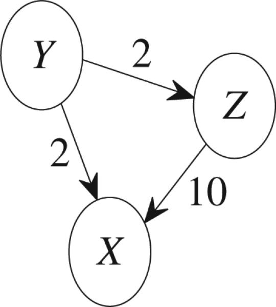
Connectivities among three time series.

Because of the above-mentioned shortcomings and/or limitations of GC, we next give a new causality definition of multivariate time series. Let us consider the following general model:

$$\{\begin{array}{c}{X}_{1,t}=\sum _{j=1}^m{a}_{11,j}{X}_{1,t-j}+\cdots +\sum _{j=1}^m{a}_{1n,j}{X}_{n,t-j}+{\eta }_{1,t}\hfill \\ X_{2,t}=\sum _{j=1}^m{a}_{21,j}{X}_{1,t-j}+\cdots +\sum _{j=1}^m{a}_{2n,j}{X}_{n,t-j}+{\eta }_{2,t}\hfill \\ ⋮\hfill \\ X_{n,t}=\sum _{j=1}^m{a}_{n1,j}{X}_{1,t-j}+\cdots +\sum _{j=1}^m{a}_{nn,j}{X}_{n,t-j}+{\eta }_{n,t}\hfill \end{array}\phantom{\}}$$ (16)

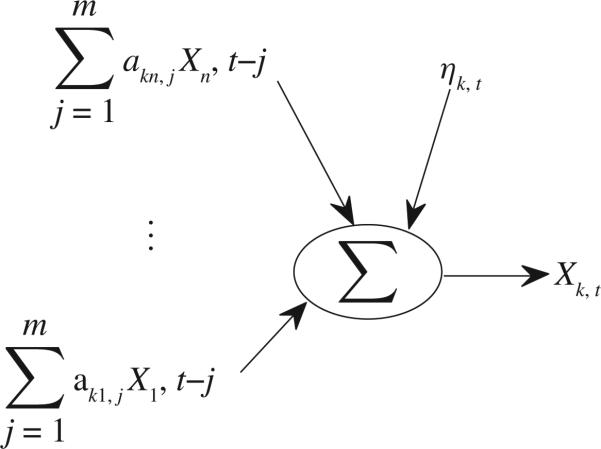
where X_i(i = 1, . . . , n) are n time series, t = 0, 1, . . . , N, η_i has zero mean and variance of ${\sigma }_{{\eta }_i}^2$ and σ_ηiηk = cov(η_i, η_k), i, k = 1, . . . , n. Based on (16), Fig.4 clearly shows contributions to X_k,t, which include ${\sum }_{j=1}^m{a}_{k1,j}{X}_{1,t-j},\dots ,{\sum }_{j=1}^m{a}_{kn,j}{X}_{n,t-j}$ and the noise term η_k,t where the influence from ${\sum }_{j=1}^m{a}_{kk,j}{X}_{k,t-j}$ is causality from X_k's own past values. Each contribution plays an important role in determining X_k,t . If ${\sum }_{j=1}^m{a}_{ki,j}{X}_{i,t-j}$ occupies a larger portion among all those contributions, then X_i has stronger causality on X_k, or vice versa. Thus, a good definition for causality from X_i to X_k in time domain should be able to describe what proportion X_i occupies among all these contributions. This is a general guideline for proposing any causality method (i.e., all contributions must be considered). For (11), let us define

$${\stackrel{‒}{\eta }}_t\stackrel{\Delta }{=}{a}_{12,1}{\eta }_{2,t-1}+{\eta }_{1,t}$$ (17)

which is the summation of two noise terms and each noise term makes contributions to $\stackrel{‒}{\eta }$. To describe what proportion η₂ occupies in $\stackrel{‒}{\eta }$, we define

$$\frac{a_{12,1}^2\sum _{t=1}^N{\eta }_{2,t-1}^2}{a_{12,1}^2\sum _{t=1}^N{\eta }_{2,t-1}^2+\sum _{t=1}^N{\eta }_{1,t}^2}=\frac{a_{12,1}^2{\sigma }_{{\eta }_2}^2}{a_{12,1}^2{\sigma }_{{\eta }_2}^2+{\sigma }_{{\eta }_1}^2}$$ (18)

which is the same as the GC defined in (13). Therefore, here, in nature, GC is actually defined based on the noise (17) and follows the above guideline. Motivated by this idea as well as (i) of Property 1, we can naturally extend the noise (17) to the kth equation of (16) and define a new direct causality from X_i to X_k as follows:

$$n_{X_i\stackrel{\mathrm{D}}{\to }{X}_k}=\frac{\sum _{t=m}^N{\left(\sum _{j=1}^m{a}_{ki,j}{X}_{i,t-j}\right)}^2}{\sum _{h=1}^n\sum _{t=m}^N{\left(\sum _{j=1}^m{a}_{kh,j}{X}_{h,t-j}\right)}^2+\sum _{t=m}^N{\eta }_{k,t}^2}.$$ (19)

Fig. 4.

Contributions to X_k,t .

When N is large enough

$$\sum _{t=m}^N{\eta }_{k,t}^2=\sum _{t=1}^N{\eta }_{k,t}^2-\sum _{t=1}^m{\eta }_{k,t}^2=N{\sigma }_{\eta k}^2-\sum _{t=1}^m{\eta }_{k,t}^2\approx N{\sigma }_{\eta k}^2.$$

Then, (19) can be approximated as

$$\frac{\sum _{t=m}^N{\left(\sum _{j=1}^m{a}_{ki,j}{X}_{i,t-j}\right)}^2}{\sum _{h=1}^n\sum _{t=m}^N{\left(\sum _{j=1}^m{a}_{kh,j}{X}_{h,t-j}\right)}^2+N{\sigma }_{\eta k}^2}.$$ (20)

Throughout this paper, we always assume that N is large enough so that $n_{X_i\stackrel{\mathrm{D}}{\to }{X}_k}$ is always defined as (20).

When n = 2 in (16), in his early work [8] Geweke stated that GC F_X2→X1 = 0 if and only if a_{12, j} ≡ 0. According to this statement, if a_{12, j} ≡ 0, then there is no causality (or GC). If a_{12, j} ≢ 0, then there is GC. Similarly, for (20) we can make the following statement: $n_{X_2\stackrel{\mathrm{D}}{\to }{X}_1}=0$ if and only if a_{12, j} ≡ 0. If $n_{X_2\stackrel{\mathrm{D}}{\to }{X}_1}\ne 0$, then a_{12, j} ≢ 0, which implies that there is causality from X₂ to X₁. If $n_{X_2\stackrel{\mathrm{D}}{\to }{X}_1}=0$, then a_{12, j} ≡ 0 and there is no causality from X₂ to X₁ As such, the new causality $n_{X_i\stackrel{\mathrm{D}}{\to }{X}_k}$ defined in (20) extends a bivariate time series to a multivariate time series. The extension to multichannel data is very important because pairwise treatments of signals can lead to errors in the estimation of mutual influences between channels [25] and [26].

New causality based on (11) can be written as

$$n_{X_2\stackrel{\mathrm{D}}{\to }{X}_1}=\frac{\sum _{t=1}^N{\left(a_{12,1}{X}_{2,t-1}\right)}^2}{\sum _{t=1}^N{\left(a_{12,1}{X}_{2,t-1}\right)}^2+\sum _{t=1}^N{\eta }_{1,t}^2}=\frac{\sum _{t=1}^N{\left(a_{12,1}{X}_{2,t-1}\right)}^2}{\sum _{t=1}^N{\left(a_{12,1}{X}_{2,t-1}\right)}^2+N{\sigma }_{\eta 1}^2}$$ (21)

which describes what proportion X₂ occupies among two contributions in X₁ [see (11)]. Note that for (11) GC F_X2→X₁ is proposed based on (17) and describes what proportion η₂ occupies among two contributions in $\stackrel{‒}{\eta }$ [see (18)]. Thus GC actually reveals causal influence from η₂ to $\stackrel{‒}{\eta }$, but it does not reveal causal influence from X₂ to X₁ at all by noting that $\stackrel{‒}{\eta }$ is only partial information of X₁, i.e., the noise terms a_{12, 1}η_2,t–+η_1,t. Any causality definition by using only partial information of X₁ may inevitably be questionable. As such, new causality is totally different from GC. In general, we can make some key comments in the following remark.

Remark 2:

1. It is easy to see that $0\le n_{X_i\stackrel{\mathrm{D}}{\to }{X}_k}\le 1$. Moreover, it is meaningful and understandable that a larger new causality value reveals a larger causal influence for different sets of bivariate time series. Thus, in this way, the thickness of arrows in Fig. 13(a) representing the strength of the connections makes much sense. As pointed out in (i) of Remark 1, a larger GC value does not necessarily reveals a larger causal influence for different sets of bivariate time series. Hence, if one uses thickness to represent strength of connections based on GC values for different sets of bivariate time series, it may not make sense. However, unfortunately almost all researchers did in this way after calculating GC values for different sets (pairs) of bivariate time series.

2. For (14) and (15), we can get $n_{X_2\stackrel{\mathrm{D}}{\to }{X}_1}=0.110$ and 0.994, respectively. For (15), $n_{X_2\stackrel{\mathrm{D}}{\to }{X}_1}=0.994$ means that influence from the noise term η₃ to X₁ is very small and X₁ is almost completely driven by X₂. Hence, the real causality from X₂ to X₁ for (15) is very close to that for the following model:

   $$\{\begin{array}{c}{X}_{1,t}=-0.8X_{2,t-1}\hfill \\ X_{2,t}=0.8X_{2,t-1}+{\eta }_{2,t}\hfill \end{array}\phantom{\}}$$ (22)

   whose real causality from X₂ to X₁ obviously equals 1. The causality value $n_{X_2\stackrel{\mathrm{D}}{\to }{X}_1}=0.994$ correctly reveals the real causality from X₂ to X₁ for (15), which is close to 1. For (14), we can easily show that influence from the noise term η₁ to X₁ is very small compared to the causal influence from X₂ to X₁ and X₁ is almost completely driven by X₁ and X₂. Hence, the real causality from X₂ to X₁ for (14) is very close to that for the following model:

   $$\{\begin{array}{c}{X}_{1,t}=0.8X_{1,t-1}-0.8X_{2,t-1}\hfill \\ X_{2,t}=0.8X_{2,t-1}+{\eta }_{2,t}\hfill \end{array}\phantom{\}}$$ (23)

   where X₁'s past value also makes a contribution to X₁'s current value. Comparing (22) to (23), one can clearly see that the real causality from X₂ to X₁ for (23) is surely weaker than that for (22). By noting small variances of the noise terms, this is why we mention the intuitive conclusion for (14) and (15) pointed in (i) of Remark 1. The causality value $n_{X_2\stackrel{\mathrm{D}}{\to }{X}_1}=0.110$ for (14) is smaller than causality value $n_{X_2\stackrel{\mathrm{D}}{\to }{X}_1}=0.994$ for (15). This result is consistent with the above analysis. However, the GC value F_X2→X1 = 4.86 for (14) is larger than the GC value F_X2→X1 = 4.18 for (15), which violates the above analysis. In fact, from $n_{X_2\stackrel{\mathrm{D}}{\to }{X}_1}=0.110$ for (14), one can see that X₁'s past value makes a rather major contribution to X₁'s current value. But this contribution is not considered in the GC as pointed in (ii) of Property 1 where the GC value from X₂ to X₁ has nothing to do with the parameters a_11,1 and a_21,1. Therefore, the causality definition in (20) is much more reasonable, stable, and reliable than GC.
3. Consider the following two models:

   $$\{\begin{array}{c}{X}_{1,t}=-0.99X_{2,t-1}+{\eta }_{1,t}\hfill \\ X_{2,t}=0.99X_{1,t-1}+0.1X_{2,t-1}+{\eta }_{2,t}\hfill \end{array}\phantom{\}}$$ (24)

   and

   $$\{\begin{array}{c}{\stackrel{‒}{X}}_{1,t}=-0.99{\stackrel{‒}{X}}_{2,t-1}+{\stackrel{‒}{\eta }}_{1,t}\hfill \\ {\stackrel{‒}{X}}_{2,t}=0.1{\stackrel{‒}{X}}_{2,t-1}+{\stackrel{‒}{\eta }}_{2,t}\hfill \end{array}\phantom{\}}$$ (25)

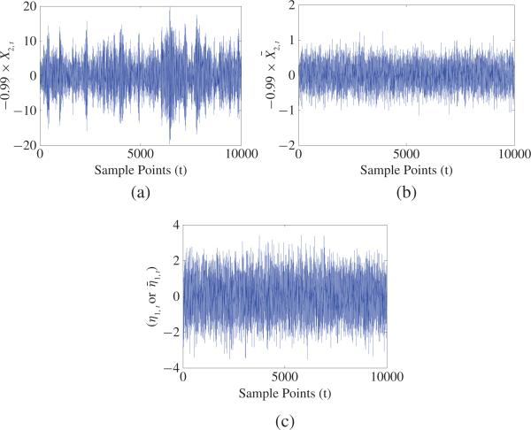
   where η₁ and η₂ are two independent white-noise processes with zero mean and variances ${\sigma }_{{\eta }_1}^2=1,{\sigma }_{{\eta }_2}^2=0.1,{\eta }_{1,t}={\stackrel{‒}{\eta }}_{1,t},{\eta }_{2,t}={\stackrel{‒}{\eta }}_{2,t}$ and the initial conditions X_{1, 0} = X̄_{1, 0} and X_{2, 0} = X̄_{2, 0}. We can obtain F_X2→X1 = 0.092 for both (24) and (25), $n_{X_2\stackrel{\mathrm{D}}{\to }{X}_1}=0.964$ for (24), and $n_{X_2\stackrel{\mathrm{D}}{\to }{X}_1}=0.090$ for (25). Fig. 5 shows trajectories –0.99X₂, –0.99X̄₂ and η₁ for one realization of (24) and (25). From Fig. 5(a) and (c), one can clearly see that amplitudes of –0.99X₂ are much larger than that of η₁ and the contribution from –0.99X₂, t–1 occupies much larger portion compared to that from η₁, t, as a result, the causal influence from X₂ to X₁ occupies a major portion compared to the influence from η₁ and the real strength of causality from X₂ to X₁ should have higher value. This fact is real. Our causality value $n_{X_2\stackrel{\mathrm{D}}{\to }{X}_1}=0.964$ for (24) is consistent with this fact. Similarly, from Fig. 5(b) and (c), one can clearly see that amplitude of –0.99X̄₂ is much smaller than that of η₁ and the contribution from –0.99X̄_{2, t–1} occupies much smaller portion compared to that from η_{1, t}, as a result, the causal influence from X̄₂ to X̄₁ occupies a rather small portion compared to the influence from η₁ and the real strength of causality from X̄₂ to X̄₁ should have a smaller value. This fact is also real. Our causality $n_{X_2\stackrel{\mathrm{D}}{\to }{X}_1}=0.090$ for (25) is consistent with this fact. However, GC always equals 0.092 for both of (24) and (25) and does not reflect such kind of changes at all, and violates the above two real facts.

4. For the two specific cases in (iii) of Property 1 and for any nonzero a_12,j, we have F_X2→X1 = 0 for (2). However, one can easily check $n_{X_2\stackrel{\mathrm{D}}{\to }{X}_1}\ne 0$ if X₂ ≢ 0, that is, there is real causality. Thus, GC F_X2→X1 = 0 does not necessarily imply no real causality, but new causality $n_{X_2\stackrel{\mathrm{D}}{\to }{X}_1}=0$ must imply no real causality (no GC). So, new causality reveals real causality more correctly than GC.

5. Once (16) is evaluated based on the n time series X₁, . . . , X_n, from (20) the direct bidirectional causalities between any two channels can be obtained. This process can save much computation time compared with the remodeling and recomputation by using conditional GC to compute the direct causality.

6. Based on this definition, one may define the indirect causality from X_i to X_k via X_l as follows:

   $$n_{X_i\stackrel{\mathrm{ID}}{\to }{X}_k\text{via}{X}_l}=n_{X_i\stackrel{\mathrm{D}}{\to }{X}_l}\times n_{X_l\stackrel{\mathrm{D}}{\to }{X}_k}.$$

   This cascade property does not hold for the previous GC definition as discussed in (iii) of Remark 1.
7. Given any route $R:X_i\to X_{l_1}^{\prime }\to X_{l_2}^{\prime }\to \cdots ,\to X_{l_h}^{\prime }\to X_k$ where $\{X_{l_1}^{\prime },\dots ,X_{l_h}^{\prime }\}\subseteq \{X_1,\dots ,X_n\}-\{X_i,X_k\}$, the indirect causality from X_i to X_k via this route R may be defined as

   $$n_{X_i\stackrel{\mathrm{ID}}{\to }{X}_k\text{via route}R}=n_{X_i\stackrel{\mathrm{D}}{\to }{X}_{l_1}^{\prime }}\times \prod _{s=1}^{h-1}{n}_{X_{l_s}^{\prime }\stackrel{\mathrm{D}}{\to }{X}_{l_{s+1}}^{\prime }}\times n_{X_{l_h}^{\prime }\stackrel{\mathrm{D}}{\to }{X}_k}.$$ (26)

   Let S_ik be the set of all such kind of routes, we may define the total causality from X_i to X_k as

   $$n_{X_i\stackrel{\mathrm{T}}{\to }{X}_k}=n_{X_i\stackrel{\mathrm{D}}{\to }{X}_k}+\sum _{R\in S_{ik}}{n}_{X_i\stackrel{\mathrm{ID}}{\to }{X}_k\text{via route}R}.$$ (27)

   Let n_Xi→Xk be the causality calculated based on the estimated AR model of the pair (X_i, X_k). The exact relationship between n_Xi→Xk and $n_{X_i\stackrel{\mathrm{T}}{\to }{X}_k}$ in (27) keeps unknown to us.

8. For the three time series as shown in Fig. 3, conditional GC can help to obtain the direct causality from Y to X (i.e., $F_{Y\stackrel{\mathrm{D}}{\to }X}$). As a result, the indirect causality from Y to X via Z (i.e., $F_{Y\stackrel{\mathrm{ID}}{\to }X\text{via}Z}$) equals $F_{Y\stackrel{\mathrm{T}}{\to }X}-F_{Y\stackrel{\mathrm{D}}{\to }X}$, where $F_{Y\stackrel{\mathrm{T}}{\to }X}$ is the total causality from Y to X. For multiple time series, given a route, one may not obtain the indirect causality based on previous GC definition. For example, in Fig. 6 the indirect causality via the route R’ : Y → W → Z → X cannot be obtained based on previous GC definition. However, using (26) we can get the indirect causality via the route R’ .

Fig. 13.

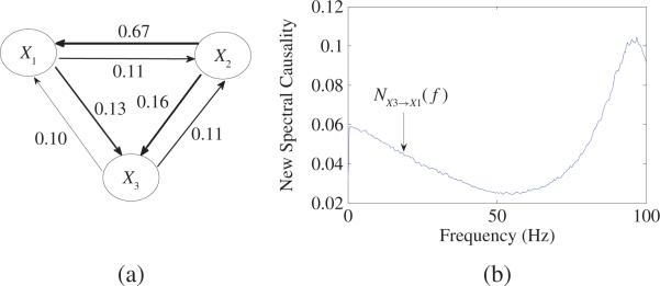
(a) Results of new causality based on (20) for (43) of three time series in time domain. Self-contributions are neglected. The resulting strength of the connections is schematically represented by the thickness of arrows. (b) New spectral causality from X₃ to X₁ is shown for (43) in frequency domain.

Fig. 5.

Plot of trajectories for –0.99X_2,t, –0.99X̄_2,t, and η_1,t for one realization of (24) and (25) where X_i,0 = X̄_i,0 and ${\eta }_{i,t}={\stackrel{‒}{\eta }}_{i,t}$, i = 1, 2: (a) –0.99 X_2,t 's trajectory for (24). (b) –0.99X̄_2,t 's trajectory for (25)(c) η_1,t 's or ${\stackrel{‒}{\eta }}_{1,t}’\mathrm{s}$ trajectory.

Fig. 6.

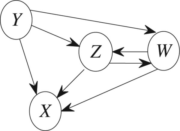
Connectivities among four time series.

For a given model, in general we do not know exactly what the real causality is. But as shown in (i)–(iv) of Remark 2, we point out that new causality value more correctly reveals the real strength of the causality than GC, and traditional GC may give misleading interpretation result.

III. GC in Frequency Domain

In the preceding section, we discussed causality in the time domain. In this section, we move to the counterpart: frequency domain. We first introduce a new spectral causality. Then we list three widely used Granger-like causality measures and point out their shortcomings and/or limitations.

Consider the general (16). Taking Fourier transformation on both side of (16) leads to

$$\{\begin{array}{c}{X}_1\left(f\right)=a_{11}\left(f\right)X_1\left(f\right)+\cdots +a_{1n}\left(f\right)X_n\left(f\right)+{\eta }_1\left(f\right)\hfill \\ X_2\left(f\right)=a_{21}\left(f\right)X_1\left(f\right)+\cdots +a_{2n}\left(f\right)X_n\left(f\right)+{\eta }_2\left(f\right)\hfill \\ ⋮\hfill \\ X_n\left(f\right)=a_{n1}\left(f\right)X_1\left(f\right)+\cdots +a_{nn}\left(f\right)X_n\left(f\right)+{\eta }_n\left(f\right)\hfill \end{array}\phantom{\}}$$ (28)

where

$$a_{lj}\left(f\right)=\sum _{k=1}^m{a}_{lj,k}{e}^{-i2\pi fk},i=\sqrt{-1},l,j=1,\dots ,n.$$ (29)

From (28), one can see that contributions to X_k(f) include not only a_k1(f)X₁(f), . . . , a_kk–1(f)X_k–1(f) a_kk+1(f)X_k+1(f), . . . , a_kn(f)X_n(f) and the noise term η_k(f), but also a_kk(f)X_k(f). Fig. 7 describes the contributions to X_k(f), which include a_k1(f)X₁(f), . . . , a_kn(f)X_n(f) and the noise term η_k(f) where the influences from a_kk(f)X_k(f) are causality from X_k's own past contribution. So, it motivates us to define a new direct causality from X_i to X_k in the frequency domain as follows:

$$N_{X_i\stackrel{\mathrm{D}}{\to }{X}_k}\left(f\right)=\frac{{\mid a_{ki}\left(f\right)\mid }^2{S}_{X_i{X}_i}\left(f\right)}{{\mid a_{k1}\left(f\right)\mid }^2{S}_{X_1{X}_1}\left(f\right)+\cdots +{\mid a_{kn}\left(f\right)\mid }^2{S}_{X_n{X}_n}\left(f\right)+{\sigma }_{\eta k}^2}$$ (30)

i, k = 1, . . . , n, i ≠ k, where S_XlXl(f) is the spectrum of X_l, l = 1, . . . , n. Similar to previous new causality definition, the causality defined in (30) is called by new spectral causality.

Fig. 7.

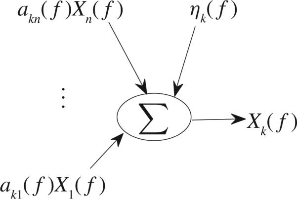
Contributions to X_k(f).

Remark 3:

1. It is easy to see that $0\le N_{X_i\stackrel{\mathrm{D}}{\to }{X}_k}\left(f\right)\le 1.N_{X_i\stackrel{\mathrm{D}}{\to }{X}_k}\left(f\right)\equiv 0$ if and only if a_ki(f) ≡ 0, which means all coefficients a_{ki, 1}, . . . , a_ki,m are zeros. $N_{X_i\stackrel{\mathrm{D}}{\to }{X}_k}\left(f\right)\equiv 1$ if and only if ${\sigma }_{{\eta }_k}^2=0$ and a_kj(f) ≡ 0, j = 1, . . . , n, j ≠ i, which means there is no noise term η_k and all coefficients a_kj,1, . . . , a_kj,m are zeros j = 1, . . . , n, j ≠ i, i.e., the kth equality in (28) can be written as

   $$X_{k,t}=\sum _{j=1}^m{a}_{ki,j}{X}_{i,t-j}$$

   from which one can see that X_k is completely driven by X_i's past values.
2. Once (16) is evaluated based on the n time series, from (30) the direct bidirectional causalities between any two channels can be obtained. Based on this definition, the indirect causality from X_i to X_k via X_l may be defined as

   $$N_{X_i\stackrel{\mathrm{ID}}{\to }{X}_k\text{via}{X}_l}\left(f\right)=N_{X_i\stackrel{\mathrm{D}}{\to }{X}_l}\left(f\right)\times N_{X_l\stackrel{\mathrm{D}}{\to }{X}_k}\left(f\right).$$
3. Given any route $R:X_i\to X_{l_1}^{\prime }\to X_{l_2}^{\prime }\to \cdots ,\to X_{l_h}^{\prime }\to X_k$ where $\{X_{l_1}^{\prime },\dots ,X_{l_h}^{\prime }\}\subseteq \{X_1,\dots ,X_n\}-\{X_i,X_k\}$, the indirect causality from X_i to X_k via this route R may be defined as

   $$N_{X_i\stackrel{\mathrm{ID}}{\to }{X}_k\text{via route}R}\left(f\right)=N_{X_i\stackrel{\mathrm{D}}{\to }{X}_{l_1}^{\prime }}\left(f\right)\times \prod _{s=1}^{h-1}{I}_{X_{l_s}^{\prime }\stackrel{\mathrm{D}}{\to }{X}_{l_{s+1}}^{\prime }}\left(f\right)\times N_{X_{l_h}^{\prime }\stackrel{\mathrm{D}}{\to }{X}_k}\left(f\right).$$

Let S_ik be the set of all such routes, we may define the total causality from X_i to X_k is

$$N_{X_i\stackrel{\mathrm{T}}{\to }{X}_k}\left(f\right)=N_{X_i\stackrel{\mathrm{D}}{\to }{X}_k}\left(f\right)+\sum _{R\in S_{ik}}{N}_{X_i\stackrel{\mathrm{ID}}{\to }{X}_k\text{via route}R}\left(f\right).$$ (31)

Let N_Xi→Xk(f) be the causality value calculated based on estimated AR model of the pair (X_i, X_k) in frequency domain. The exact relationship between N_Xi→Xk(f) and $N_{X_i\stackrel{\mathrm{T}}{\to }{X}_k}\left(f\right)$ in (31) is unknown to us so far.

In the literature, there are several other measures to define causality of neural connectivity in the frequency domain. In the following, we will introduce these measures and point out their shortcomings and/or limitations.

1) Spectral GC ( [6], [8], [24], [25], [27]): Given the bivariate (2), the Granger casual influence from X₂ to X₁ is defined by

$$I_{X_2\to X_1}\left(f\right)=-\text{log}\left(1-\frac{\left({\sigma }_{{\eta }_2}^2-\frac{{\sigma }_{{\eta }_1{\eta }_2}^2}{{\sigma }_{{\eta }_1}^2}\right){\mid H_{12}\left(f\right)\mid }^2}{S_{X_1{X}_1}}\right)\in [0,+\infty )$$ (32)

where the transfer function is H(f) = A^–1(f) whose components are

$$\begin{array}{cc}\hfill H_{11}\left(f\right)& =\frac{1}{\text{det}\left(A\right)}{\stackrel{‒}{a}}_{22}\left(f\right),H_{12}\left(f\right)=-\frac{1}{\text{det}\left(A\right)}{\stackrel{‒}{a}}_{12}\left(f\right)\hfill \\ \hfill H_{21}\left(f\right)& =-\frac{1}{\text{det}\left(A\right)}{\stackrel{‒}{a}}_{21}\left(f\right),H_{22}\left(f\right)=\frac{1}{\text{det}\left(A\right)}{\stackrel{‒}{a}}_{11}\left(f\right)\hfill \end{array}$$ (33)

$A={\left[{\stackrel{‒}{a}}_{ij}\right]}_{2\times 2},{\stackrel{‒}{a}}_{kk}\left(f\right)=1-{\sum }_{j=1}^m{a}_{kk,j}{e}^{-i2\pi fj},k=1,2,{\stackrel{‒}{a}}_{hl}\left(f\right)=-{\sum }_{j=1}^m{a}_{hl,j}{e}^{-i2\pi fj},h,l=1,2,h\ne l$.

This definition has shortcomings and/or limitations as shown in the following remark.

Remark 4:

1. The same problems exist as in (i) and (iii) of Remark 1.

2. For the two specific cases in (iii) of Property 1 and for any coefficients a_11,j, a_12,j, a_21,j, a_22,j, we can check I_X2 → X₁ (f) ≡ 0 based on (32). However, one can easily check $N_{X_2\stackrel{\mathrm{D}}{\to }{X}_1}\left(f\right)\ne 0$ for (2) if a₁₂(f)X₂(f) ≠ 0: that is, there is real causality. Thus spectral GC I_X2 → X₁ (f) = 0 does not necessarily imply no real causality for the given frequency f, but new spectral causality $N_{X_2\stackrel{\mathrm{D}}{\to }{X}_1}\left(f\right)=0$ must imply no real causality (of course, no spectral GC). As such, new spectral causality definition reveals real causality more correctly than spectral GC.

3. From in (17.22), (17.23), (32), and (33) above, we can derive

   $$I_{X_2\to X_1}\left(f\right)=\frac{\Delta }{{\sigma }_{{\eta }_1}^2{\mid {\stackrel{‒}{a}}_{22}\left(f\right)\mid }^2-2{\sigma }_{{\eta }_1{\eta }_2}\mathrm{Re}\left({\stackrel{‒}{a}}_{12}\left(f\right){\stackrel{‒}{a}}_{22}^{\ast }\left(f\right)\right)+\frac{{\sigma }_{{\eta }_1{\eta }_2}^2}{{\sigma }_{{\eta }_1}^2}{\mid {\stackrel{‒}{a}}_{12}\left(f\right)\mid }^2+\Delta }$$ (34)

   where $\Delta =\left({\sigma }_{{\eta }_2}^2-{\sigma }_{{\eta }_1{\eta }_2}^2∕{\sigma }_{{\eta }_1}^2\right){\mid {\stackrel{‒}{a}}_{12}\left(f\right)\mid }^2$. Its detailed derivation is omitted here for space reason. One can see that I_X2→X1(f) has nothing to do with ā₁₁(f) and ā₂₁(f), or, the real casuality from X₂ to X₁ in (2) has nothing to do with a_{11, j} and a_{21, j} . This is not true [similar to the analysis in (ii) and (iii) of Remark 2]. Thus, in general, spectral GC in (32) does not disclose the real casual influence at all.

4. GC was extended to conditional GC in frequency domain [6] and [8]. So, there exists the same problem as in (ii) above for conditional spectral GC.

2) PDC [14] and [28]: Let

$${\stackrel{‒}{a}}_{ij}\left(f\right)={\delta }_{ij}-a_{ij}\left(f\right)$$ (35)

where a_ij(f) is as in (29), and δ_ij = 1 if i = j and 0 otherwise. Then in (16), PDC is defined to show frequency domain causality from X_j to X_i at frequency f as

$${\pi }_{i\leftarrow j}\left(f\right)=\frac{{\stackrel{‒}{a}}_{ij}\left(f\right)}{\sqrt{\sum _{i=1}^n{\mid {\stackrel{‒}{a}}_{ij}\left(f\right)\mid }^2}},i,j=1,\dots ,n.$$ (36)

The PDC π_i←j(f) represents the relative coupling strength of the interaction of a given source, signal X_j, with regard to signal X_i, as compared with all of X_j's causing influences on other signals. Thus, PDC ranks the relative strength of causal interaction with respect to a given signal source and satisfies the following properties:

$$0\le {\mid {\pi }_{i\leftarrow j}\left(f\right)\mid }^2\le 1\text{and}\sum _{i=1}^n{\mid {\pi }_{i\leftarrow j}\left(f\right)\mid }^2=1,j=1,\dots ,n.$$

π_i←i(f) represents how much of X_i's own past contributes to the evolution on itself that is not explained by other signals (see [29]). Fig. 8 describes contributions of signal X_j to all signals X₁, . . . , X_n and can help the reader to better understand the definition of PDC. Comparing Fig. 8 with Fig. 7, one can see that these two figures have different structures. It is notable that π_i←j(f) = 0 (i ≠ j) can be interpreted as absence of functional connectivity from signal X_j to signal X_i at frequency f. Hence, PDC can be used to multivariate time series to disclose whether or there exists casual influence from signal X_j to signal X_i. However, some researchers [30] already noted that PDC is hampered by a number of problems. In the following remark, we point out its shortcomings and/or limitations in a particular way.

Fig. 8.

X_j's contributions to all signals X_i, i = 1, 2, . . . , n.

Remark 5:

1. Note that π_i←i(f) represents how much of X_i's own past contributes to the evolution on itself (see [29]). Then, π_i←i(f) = 0 means no X_i's own past contributes to the evolution on itself. However, π_i←i(f) = 0 implies ā_ii(f) = 0, that is, 1 – a_ii(f) = 0 or a_ii(f) = 1(≠ 0), which means that there is X_i's own past contributes to the evolution on itself. A contradiction! On the other hand, π_i←i(f) = 1 implies ā_ki(f) = 0 (i.e., a_ki(f) = 0), k = 1, 2, . . . , n, k ≠ i, and ā_ii(f) ≠ 0 (i.e., a_ii ≠ 1). Given a frequency f, now we further assume X_j(f) = X_i(f) = 1 and a_ij(f) = 1, a_ii(f) = 0.01 for some j ≠ i. Then, a_ij(f)X_j(f) = 1 and a_ii(f)X_i(f) = 0.01. Thus, based on the ith equality of (28) we know that X_i's own past contributes to the evolution on itself (i.e., a_ii(f)X_i(f) = 0.01) is much smaller than X_j's past contribution to X_i's evolution (i.e., a_ij(f)X_j(f) = 1) and can even be ignored. Thus, the number 1(= π_i←i(f)) is not meaningful and PDC π_i←i(f) is not reasonable.

2. High PDC π_i←j(f), j ≠ i, near 1, indicates strong connectivity between two neural structures (see [21]). This is not true in general. For example, assume π_1←j(f) = 1(j ≠ 1, 2), which implies ā_kj(f) = 0, k = 2, . . . , n and ā_1j(f) ≠ 0 (or a_1j(f) ≠ 0). Given a frequency f, now we further assume X_j(f) = X₂(f) = 1 and a₁₂(f) = 1, a_1j(f) = 0.01. Then, a_1j(f)X_j(f) = 0.01 and a₁₂(f)X₂(f) = 1. Thus, based on the first equality of (28) we know that X_j's past contributes to X₁'s evolution (i.e., a_1j(f)X_j(f) = 0.01) is much smaller than X₂'s past contribution to X₁'s evolution (i.e., a₁₂(f)X₂(f) = 1) and can even be ignored. This demonstrates that there exists a very weak connectivity between X_j and X₁. However, π_1←j(f) = 1 indicates strong connectivity between X_j and X₁. A contradiction!

3. Small PDC π_i←k(f) does not means causal influence from X_k to X_i is small. For example, assume a_ik(f) = 0, i = 2, . . . , n and ā_1k(f) = 0.1. Then, in terms of (36) one can see that π_1←k(f) ≈ 0.1, which is a small number. However, note the first equality of (28), if X_k(f) is a big number such that ā_1k(f)X_k(f) is much larger than any one of ā_1j(f)X_j(f), j ≠ k. Then, X_k has major causal influence on X₁ compared with other signals on X₁.

4. π_i←j(f) > π_i←k(f) cannot guarantee that causality from X_j to X_i is larger than that from X_k to X_i where j ≠ i, k ≠ i. Actually (ii) and (iii) above support this statement.

5. Consider (2) and further assume a_21,j = 0, j = 1, . . . , m. One can clearly see that π_1←2(f) has nothing to do with ā₁₁(f), or, the real casual influence from X₂ to X₁ in (2) has nothing to do with a_11,j, j = 1, . . . , m. This is not true [similar to the analysis in (ii) and (iii) of Remark 2].

6. The same problems as in (i) above ~(v) exist for a form of PDC called generalized PDC (GPDC) [31], [32].

3) RPC [15]: From (28) it follows that the transfer function H(f) = [H_ij(f)] = A^–1(f) where A = [ā_ij(f)]_n×n and ā_ij(f) is as (35). When all noise terms are mutually uncorrelated, a simple RPC is defined as

$$R_{i\leftarrow j}\left(f\right)=\frac{{\mid H_{ij}\left(f\right)\mid }^2{\sigma }_{{\eta }_j}^2}{S_{X_i{X}_i}\left(f\right)}$$ (37)

where the power spectrum

$$S_{X_i{X}_i}\left(f\right)=\sum _{j=1}^n{\mid H_{ij}\left(f\right)\mid }^2{\sigma }_{{\eta }_j}^2,(i=1,\dots ,n).$$ (38)

Equation (38) indicates that the power spectrum of X_i,t at frequency f can be decomposed into n terms ${\mid H_{ij}\left(f\right)\mid }^2{\sigma }_{{\eta }_j}^2$, (j = 1, . . . , n), each of which can be interpreted as the power contribution of the jth innovation η_j,t transferring to X_i,t via the transfer function H_ij(f). Thus, ${\mid H_{ij}\left(f\right)\mid }^2{\sigma }_{{\eta }_j}^2$ can be regarded as the power contribution of the innovation η_j,t on the power spectrum of X_i,t. RPC R_i←j(f) defined in (37) can be regarded as a ratio of the power contribution of the innovation η_j,t on the power spectrum of X_i,t to the power spectrum S_XiXi(f). Hence, RPC gives a quantitative measurement of the strength of every connection for each frequency component and always ranges from 0 to 1. The ratio is used to define X_j's past contributes to X_i's evolution. Fig. 9 describes contributions to signal X_i's evolution from all signals X_k's past values (k = 1, . . . , n) and can help the reader to better understand the definition of RPC. Comparing Fig. 9 with Fig. 8, one can see that these two figures have different structures. Although RPC can be applied to multivariate time series, it has its shortcomings and/or limitations as pointed out in the following remark.

Fig. 9.

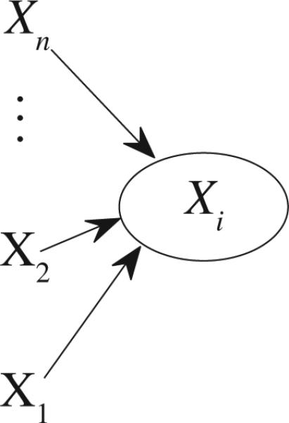
Past contributions to X_i's evolution from all signals X_j, j = 1, 2, . . . , n.

Remark 6:

1. RPC R_i←j(f) defined in (37) can only be regarded as a ratio of the power contribution of the innovation η_j,t on the power spectrum of X_i,t to the power spectrum S_XiX_i(f). In the literature, all researchers who use RPC to study neural connectivity view the ratio as X_j's past contribution to X_i's evolution. Unfortunately, the ratio cannot be used to define X_j's past contribution to X_i's evolution. It does not disclose real causal influence from X_j to X_i at all. For multivariate time series, R_i←j(f) = 0 does not mean no causal influence from X_j to X_i, R_i←j(f) = 1 does not mean strong causality from X_j to X_i. For example, given a frequency f, let the transfer function H(f) = [H_ij(f)] = A^–1(f) satisfy H_1j(f) = 0 and ā_1j(f) ≠ 0 (or a_1j(f) ≠ 0), j ≠ 1. H_1j(f) = 0 indicates R_1←j(f) = 0. However, from the first equality of (28) and a_1j(f) ≠ 0, one can see that there exists causality from X_j to X₁. Let the transfer function H(f) = [H_ij(f)] = A^–1(f) satisfy H_1j(f) ≠ 0, H_1k(f) = 0, k = 1, . . . , n, k ≠ j and ā_1j(f) = 0 (or a_1j(f) = 0), j ≠ 1. From H_1j(f) ≠ 0, H_1k(f) = 0, k = 1, . . . , n, k ≠ j, it can be seen that R_1←j(f) = 1. However, from the first equality of (28) and a_1j(f) = 0, one can see that there exists no direct causality from X_j to X₁ at all. Hence, RPC value R_i←j(f) is not meaningful as far as causality from X_j to X_i is concerned.

2. In general, RPC R_i←j(f) in (37) is unreasonable. The same analysis as (v) of Remark 5 leads to this statement.

3. When noise terms are mutually correlated, extended RPC (ERPC) was proposed in [15], and [33]. The same problems as above (i) and (ii) exist for ERPC.

4) DTF or Normalized DTF [16]: DTF is directly based on the transfer function H(f). It is defined as (37) where ${\sigma }_{{\eta }_j}^2=1$, j = 1, . . . , n. So, the same problems as (i) and (ii) of Remark 6 exist for normalized DTF.

In conclusion, for four widely used Granger or Granger-like causlity measures (spectral GC, PDC, RPC, and DTF), we clearly point out their inherent shortcomings and/or limitations. One of reasons for causing those shortcomings and/or limitations is the use of the transfer function H(f) or its inverse matrix. In fact, Fig. 7 gives a rather intuitive description for the contributions to X_k(f), which are summations of all causal influence terms a_k1(f)X₁(f), . . . , a_kn(f)X_n(f) and the instantaneous causal influence noise term η_k(f) where a_kk(f)X_k(f) is the causal influence from X_k's past value. $N_{X_i\stackrel{\mathrm{D}}{\to }{X}_k}\left(f\right)$ defined in (30) describes how much causal influence of all influences on X_k(f) comes from X_i(f). Thus, new spectral causality defined in (30) is mathematically rather reasonable and understandable. Any other causality measure not directly depending on all these causal influence terms and the instantaneous causal influence noise term may not truly reveal causal influence among different channels. Note that the new definition is totally different from all existing Granger or Granger-like causality measures which are directly based on the transfer function (or its inverse matrix) of the AR model. The difference mainly lies in two aspects: 1) the element H_ij(f) of the transfer function H(f) is totally different from a_ij(f) in (28) and as a result any causality measure based on H(f) may not reveal real causality relations among different channels, and 2) as pointed out in (iii) of Remark 4, (v) of Remark 5, and (ii) of Remark 6, Granger or Granger-like causality measures use only partial information and some information is missing [e.g., I_X2→X1(f) in (34) has nothing to do with ā₁₁(f) or –a₁₁(f)] unlike new spectral causality defined as (30) in which all powers S_XiX_i (i = 1, . . . , n) (including all available information) are adopted. As such, spectral GC, PDC, RPC, DTF, and many other extended or variant forms like GPDC [31], extended RPC (ERPC) [33], normalized DTF [16], direct directed transfer function (dDTF) [34], SDTF [35], short-time direct directed transfer function (SdDTF) [17], to name a few, suffer from the loss of some important information and inevitably cannot completely reveal true causality influence among channels.

IV. Examples

In this section, we first compare our causality measures with the existing causality measures in the first four examples and in particular we show the shortcomings and/or limitations of the existing causality measures. In Examples 1–4, we always assume all noise terms are mutually independent and normal distribution with variance of 1 except for Example 4 which has a variance of 0.3. In the last example, we then conduct event-related causality analysis for a patient who suffered from seizure in left temporal lobe and was asked to recognize pictures viewed. In this example, we calculate new spectral causality, spectral GC, PDC, and RPC for two intracranial EEG channels where one channel is from left temporal lobe and the other channel is from right temporal lobe. The simulation results show that all measures clearly reveal causal information flow from right side to left side, but new spectral causality result reflects event-related activity very well and spectral GC, PDC, and RPC results are not interpretable and misleading.

Example 1: Comparison between spectral GC and new spectral causality. Consider the following model:

$$\{\begin{array}{c}{X}_{1,t}=a_{11,1}{X}_{1,t-1}-0.8X_{2,t-1}+{\eta }_{1,t}\hfill \\ X_{2,t}=0.8X_{2,t-1}+{\eta }_{2,t}.\hfill \end{array}\phantom{\}}$$ (39)

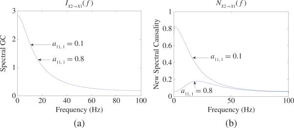
We consider two cases: a_{11, 1} = 0.1 and a_{11, 1} = 0.8. Obviously, X₂ should have different causal influence on X₁ in these two cases. Fig. 10(b) shows the new spectral causality results in these two cases from which one can see that X₂ has totally different causal influence on X₁ in these two cases. However, based on (34), X₂ has the same GC on X₁ in these two cases [see Fig. 10(a)] because (34) has nothing to do with the coefficient a_{11, 1}. Hence, we confirm that in general spectral GC may not reflect real causal influence between two neurons and may lead to wrong interpretation.

Fig. 10.

(a) Spectral GC results: I_X2→X1(f) based on (34) for (39) of two time series in two cases: a_{11, 1} 0.1 and a_{11, 1} = 0.8. (b) New spectral causality results: N_X2→X1(f) for (39).

Example 2: Comparison between new spectral causality and PDC. Consider the following model with three time series:

$$\{\begin{array}{c}{X}_{1,t}=0.1X_{1,t-1}-0.2X_{2,t-1}-0.2X_{3,t-1}+{\eta }_{1,t}\hfill \\ X_{2,t}=-0.1X_{1,t-1}+0.8X_{2,t-1}-0.2X_{3,t-1}+{\eta }_{2,t}\hfill \\ X_{3,t}=1.5X_{1,t-1}-0.2X_{2,t-1}+0.8X_{3,t-1}+{\eta }_{3,t}.\hfill \end{array}\phantom{\}}$$ (40)

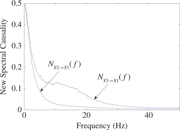
For (40), it is easy to check that π_1←2(f) = π_1←3(f) for any frequency f > 0 based on PDC definition of (36). This is not true. The reason is that X₂(f) ≠ X₃(f) for most frequency f > 0 and, as a result, ā₁₂(f)X₂(f) ≠ ā₁₃(f)X₃(f) by noting ā₁₂(f) = ā₁₃(f) for any frequency f > 0. Thus, in the frequency domain, X₂ and X₃ should have different causal influence on X₁. The new spectral causality plotted in Fig. 11 shows that the causality from X₂ to X₁ is indeed totally different from that from X₃ to X₁ for most frequency f > 0. So, we confirm that in general PDC value may not reflect real causality between two neurons and may be misleading.

Fig. 11.

New spectral causality results: $N_{X_2\stackrel{\mathrm{D}}{\to }{X}_1}\left(f\right)$ and $N_{X_3\stackrel{\mathrm{D}}{\to }{X}_1}\left(f\right)$ for (40).

Example 3: Comparison between new spectral causality and RPC. First consider the following model with three time series:

$$\{\begin{array}{c}{X}_{1,t}=0.5X_{1,t-1}-0.2X_{1,t-2}+0.5X_{2,t-1}+{\eta }_{1,t}\hfill \\ X_{2,t}=0.8X_{1,t-1}-0.5X_{1,t-2}+0.2X_{2,t-1}+0.4X_{3,t-1}+{\eta }_{2,t}\hfill \\ X_{3,t}=0.6X_{1,t-1}-0.5X_{3,t-1}+0.5X_{3,t-2}+{\eta }_{3,t}.\hfill \end{array}\phantom{\}}$$ (41)

From (41), one can get the transfer function H(f) = A^–1(f), H₁₁(f) = (1 – 0.2e^–i2πf)(1 + 0.5e^–i2πf – 0.5e^–i4πf)/det(A), H₁₂(f) = 0.5e^–i2πf (1 + 0.5e^–i2πf – 0.5e^–i4πf)/det(A), H₁₃(f) = 0.5e^–i2πf × 0.4e^–i2πf/det(A). We compute

$$R_{1\leftarrow 3}\left(f\right)=\frac{{\mid H_{13}\left(f\right)\mid }^2}{{\mid H_{11}\left(f\right)\mid }^2+{\mid H_{12}\left(f\right)\mid }^2+{\mid H_{13}\left(f\right)\mid }^2}.$$ (42)

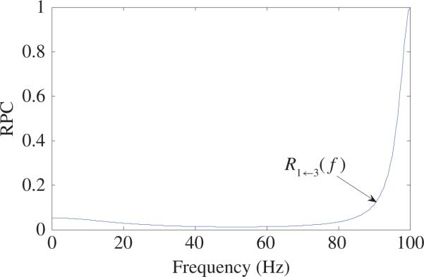
The curve of RPC R_1←3(f) based on (42) is shown in Fig. 12 from which one can see that there always exists direct causal influence from X₃ to X₁ for f > 0. Especially, when f = 100 Hz, R_1←3(100) = 1, which indicates that there is very strong direct causal influence from X₃ to X₁. However, from the first equality of (41), one can see that there is no real direct causal influence from X₃ to X₁ at all.

Fig. 12.

Curve of RPC R_1←3(f) calculated based on (42).

We then consider the following model with three time series:

$$\{\begin{array}{c}{X}_{1,t}=0.2X_{1,t-1}-0.2X_{1,t-2}+0.8X_{2,t-1}-0.4X_{3,t-2}+{\eta }_{1,t}\hfill \\ X_{2,t}=0.3X_{1,t-1}-0.2X_{1,t-2}-0.6X_{2,t-1}+0.5X_{3,t-1}+0.3X_{3,t-2}+{\eta }_{2,t}\hfill \\ X_{3,t}=0.4X_{1,t-1}+0.3X_{2,t-1}-0.4X_{3,t-1}+0.3X_{3,t-2}+{\eta }_{3,t}.\hfill \end{array}\phantom{\}}$$ (43)

From (43), one can get the transfer function H(f) = A^–1(f) with H₁₃(f) = 0, ∀f > 0. As a result, RPC R_1←3(f) ≡ 0, ∀f > 0, which indicates no direct causal influence from X₃ to X₁. However, from (43) one can see that X₃ indeed has causal influence on X₁. Moreover, every two time series have bidirectional connectivities, which are shown in Fig. 13(a). Causality in frequency domain from X₃ to X₁ is plotted in Fig. 13(b), from which one can see that there always exists causal influence from X₃ to X₁ for a given frequency f > 0.

Hence, by above two models, we confirm that in general RPC value may not reflect real causal influence between two neurons and, as a result, may yield misleading results.

Example 4: Comparison among new spectral causality, conditional spectral GC, PDC, and RPC together. Consider the following model with three time series:

$$\{\begin{array}{c}{X}_{1,t}=0.3X_{1,t-1}-0.1X_{1,t-2}+0.4X_{2,t-1}-0.2X_{2,t-2}+0.3X_{3,t-1}-0.4X_{3,t-2}+{\eta }_{1,t}\hfill \\ X_{2,t}=0.3X_{1,t-1}-0.4X_{1,t-2}+0.3X_{2,t-1}-0.1X_{2,t-2}+0.4X_{3,t-1}-0.2X_{3,t-2}+{\eta }_{2,t}\hfill \\ X_{3,t}=0.4X_{1,t-1}-0.2X_{1,t-2}+0.3X_{2,t-1}-0.4X_{2,t-2}+0.3X_{3,t-1}-0.1X_{3,t-2}+{\eta }_{3,t}\hfill \end{array}\phantom{\}}$$ (44)

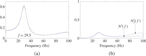
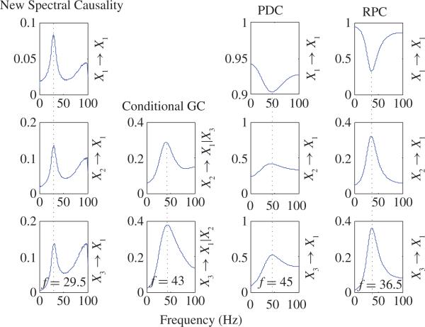
where the noise terms are normal distribution with variance of 0.3 and all noise terms are mutually independent. For each realization (200 realizations of 10 000 time points) of (44), we estimated AR model [as mentioned in (ii) of Property 1] and calculated power, new spectral causality, conditional spectral GC, PDC, and RPC values in frequency domain. Then average values across all realizations are reported in Figs. 14 and 15. Power spectra of X₁, X₂, and X₃ are plotted in Fig. 14(a), from which one can see that X₁, X₂, and X₃ have almost same power spectra across all frequencies and have an obvious peak at f = 29.5 Hz. New spectral causality, conditional spectral GC, PDC, and RPC are shown in Fig. 15. The first, third, and fourth columns in Fig. 15 shows direct new spectral causality, PDC, and RPC, respectively, from X₁ to X₁, from X₂ to X₁, and from X₃ to X₁. It is notable that new spectral causalities from X₁ to X₁, from X₂ to X₁, and from X₃ to X₁ are similar and have peaks at the same frequency of 29.5 Hz, which is consistent with the peak frequency of power spectra in Fig. 14(a). So, these new spectral causality results are rather interpretable and reasonable by noting the almost same power spectra in Fig. 14(a) for X₁, X₂, and X₃. On the contrary, conditional GC in the second cloumn of Fig. 15, PDC, and RPC (from X₂ to X₁, and from X₃ to X₁) have peaks at different frequencies which are all different from 29.5 Hz. These results are not interpretable by noting the same peak frequency (29.5 Hz) of power spectra in Fig. 14(a). More specifically, PDC and RPC (from X₁ to X₁) achieve minimum at peak frequencies of PDC and RPC (from X₂ to X₁ or from X₃ to X₁). Obviously, these results are incorrect and misleading. N(f) and N_T(f) are presented in Fig. 14(b), where $N\left(f\right)=N_{X_3\stackrel{\mathrm{D}}{\to }{X}_2}\left(f\right)\times N_{X_2\stackrel{\mathrm{D}}{\to }{X}_1}\left(f\right)$ based on (44) and N_T(f) = N_X3→X1(f) based on the estimated AR model of the pair (X₁, X₃). One can see that N_T(f) (i.e., the total causality from X₃ to X₁) is very close to N(f) (i.e., summation of causalities along all routes from X₃ to X₁) before 40 Hz. But after 40 Hz, N(f) > N_T(f). For a general model, the exact relationship between N(f) and N_T(f) is unknown.

Fig. 14.

(a) Power spectra of X₁, X₂, X₃. It can be seen that X₁, X₂, X₃ have almost same powers across all frequencies and have an obvious peak at f = 29.5 Hz. (b) $N\left(f\right)=N_{X_3\stackrel{\mathrm{D}}{\to }{X}_2}\left(f\right)\times N_{X_2\stackrel{\mathrm{D}}{\to }{X}_1}\left(f\right)$ based on (44) and N_T(f) = N_X3→X1 (f) based on the estimated AR model of the pair (X₁, X₃). One can see that N_T(f) (i.e., the total causality from X₃ to X₁) is very close to N(f) (i.e., summation of causalities along all routes from X₃ to X₁) before 40 Hz. But after 40 Hz, N(f) > N_T(f). For a general model, the exact relationship between N(f) and N_T(f) is not known.

Fig. 15.

Comparison among new spectral causality, conditional spectral GC, PDC, and RPC together. The first, third, and fourth columns show direct new spectral causality, PDC, and RPC, respectively, from X₁ to X₁, from X₂ to X₁, and from X₃ to X₁. The second column shows conditional GC. It is notable that: 1) new spectral causality from X₁ to X₁, from X₂ to X₁, and from X₃ to X₁ are similar and have peaks at the same frequence of 29.5 Hz, which is consistent with the peak frequency of power spectra [see Fig. 14(a)], and 2) conditional GC, PDC, and RPC (from X₂ to X₁, and from X₃ to X₁) have peaks at different frequencies which are all different from 29.5 Hz.

Hence, by this example, we confirm that in general spectral GC, PDC, and RPC may not reflect real causality.

Example 5: In this example, we conduct ERP analysis for one seizure patient who suffered from seizure in left temporal lobe and was asked to recognize pictures viewed. There are two sessions for testing. During the first session, stimuli was presented and evaluated for their emotional impact (valence, arousal) and autonomic effects. Stimuli were chosen that are known to activate the amygdala from functional imaging studies. A second session was a recall task in which the subject was asked to recognize pictures viewed in session 1. The subject was comfortably seated in front of a computer monitor projecting and imaging from the International Affective Picture System (IAPS) every 22 s according to the above schema. Forty images were selected that span the range of emotional valence and arousal according to previously published standards. The image was held on the screen for 6 s, and then the subject was asked to rate the image on an emotional valence (0 = not emotionally intense to 3 = extremely emotionally intense). Reaction time to the rating was measured. After rating, the screen went blank for 15 s. Twenty-four hours later, a second session was held in which pictures were presented in random order. All 40 of the previously viewed pictures as well as another 80 pictures from the IAPS with similar overall valence and arousal ratings were presented. Each image was presented for 3 s and then the patient was asked if it had been previously seen or not and to what degree of certainty this can be stated (e.g., not seen before very certain to not seen before very unsure). Reaction time to the response was measured. A blank screen followed the response for 2 s. We recorded intracranial EEG and behavioral data (response times and choices) from 16 electrodes consisting of right and left temporal depth electrodes (RTD and LTD, the locations of these electrodes can be seen in [36, Fig. 2]) composed of eight platinum/iridium alloy contacts spaced at 10 mm intervals on an XLTek EEG 128 system which digitizes each channel at 625 Hz with a 0.01–100 Hz analog band-pass digital filter. All channels (16) were referred to the scalp suture electrode. Individual stimulus response trials were visually inspected and those with artifacts were excluded from subsequent analysis. After visual inspection, the remaining analyzed data involves 7500 sample points and 78 epochs.

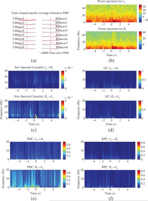
As in many researchers have done, we use the average referenced iEEG. ERP images in Fig. 16(a) clearly show cortical activity changes after stimulus onset in most channels. To study task-related causality relationship between different channels, we use the moving window technique where the window size is 150 samples (240 ms) and overlap is 75 samples (120 ms). After a complete analysis for the MVAR model order in each window by using the Akaike information criterion [37]–[39] we found the chosen order of 8 fits well and thus a common model order of 8 was applied for all windows in our data set.

Fig. 16.

(a) ERPs for eight left Macrowire channels (LMacro1–LMacro8) and eight right Macrowire channels (RMacro1–RMacro8) where average reference is applied. (b) Power spectra for LMacro4 (or L4) and RMacro5 (or R5). (c) New spectral causality results between L4 and R5. (d) GC results between L4 and R5. (e) PDC results between L4 and R5. (f) RPC results between L4 and R5.

We took R5 and L4 as an example and calculated their causality relationship based on new spectral causality, spectral GC, PDC, and RPC. The power spectra for R5 and L4 averaged over all trials are shown in Fig. 16(b), from which one clearly sees that delayed lower frequency band (<8 Hz) activities are enhanced after stimulus onset (about 250 ms time delay). This result is consistent with previous findings that theta (2–10 Hz) oscillations have been observed to be prominent during a variety of cognitive processes in both animal and human studies [40]–[44] and may play a fundamental role in memory encoding, consolidation, and maintenance [45]–[47]. Time–frequency causality [or event-related causality (see, [17])] relationship between R5 and L4 based on new spectral causality, spectral GC, PDC, and RPC are shown in Fig. 16(c)–(f) respectively, from which one can find that: 1) the causal influence from R5 to L4 is significantly enhanced after stimulus onset (about 250 ms time delay) for all four measures (we use the statistical testing framework in [17] to test significance level for each measure). But only new spectral causality discloses the enhanced frequency band (<8 Hz), which is consistent with the delayed enhanced lower frequency band (<8 Hz) activities of R5 and L4 as shown in Fig. 16(b) and thus the result should be real. The enhanced frequency bands revealed by the other measures (spectral GC, PDC, RPC) are always less than 2 Hz and the enhanced lower frequency band (2–8 Hz) activities shown in Fig. 16(b) cannot be reflected and thus these results lead to misinterpretation, and 2) the causal influence from L4 to R5 is much smaller than that from R5 to L4 for each measure. These results indicate that interaction between the pair of R5 and L4 is not symmetric and R5 has a strong directional interaction on L4. A possible reason for this phenomenon is that the patient had left temporal lobe epilepsy and therefore some of brain functions were lost, which kept information flow in left temporal lobe from normally transmitting to right temporal lobe.

Hence, by this real neurophysiological data analysis, we further verify that new spectral causality may truly reveal causal interaction between two areas and the other measures like spectral GC, PDC, and RPC cannot do and thus may lead to wrong interpretation results.

V. Conclusion

In human cognitive neuroscience, researchers are now not limited to only the study of the putative functions of particular brain regions, but are moving toward how different brain regions (such as visual cortex, parietal or frontal regions, amygdala, or hippocampus) may causally influence on each other. These causal influences with different strengths and directionalities may reflect the changing functional demands on the network to support cognitive and perceptual tasks. Direct evidence to show the existence of causality among brain regions can be achieved from the activity changes of brain regions by using brain stimulation approach. Brain stimulation affects not only the targeted local region but also the activity in remote interconnected regions. These remote effects depend on cognitive factors (e.g., task-condition) and reveal dynamic changes in interplay between brain areas. GC, one of the most popular causality measures, was initially widely used in economics and has recently received growing attention in neuroscience to reveal causal interactions for neurophysiological data. Especially in frequency domain, several variant forms of GC have been developed to study causal influences for neurophysiological data in different frequency decompositions during cognitive and perceptual tasks.

In this paper, on one hand, in time domain we defined a new causality from any time series Y to any time series X in the linear regression model of multivariate time series, which describes the proportion that Y occupies among all contributions to X (where each contribution must be considered when defining any good causality tool, otherwise the definition inevitably cannot reveal well the real strength of causality between two time series). In particular, we used one simple example to clearly show that both of new causality and GC adopt the concept of proportion, but they are defined on two different equations where one equation (for GC) is only part of the other equation (for new causality). Therefore, new causality is a natural extension of GC and has a sound conceptual/theoretical basis, and GC is not the desired causal influence at all. As such, traditional GC has many pitfalls, e.g., a larger GC value does not necessarily mean higher real causality, or vice versa; even when GC value is zero, there still exists real causality which can be revealed by new causality. Therefore, the popular traditional GC cannot reveal the real strength of causality at all, and researchers must apply caution in drawing any conclusion based on GC value. On the other hand, in frequency domain we pointed out that any causality definition based on the transfer function matrix (or its inverse matrix) of the linear regression model in general may not be able to reveal the real strength of causality between two time series. Since almost all existing spectral causality definitions are based on the transfer function matrix (or its inverse matrix) of the linear regression model, we took the widely used spectral GC, PDC, and RPC as examples and pointed out their inherent shortcomings and/or limitations. To overcome these difficulties, we defined a new spectral causality which describes the proportion that one variable occupies among all contributions to another variable in the multivariate linear regression model (frequency domain). By several simulated examples, we clearly showed that our new definitions (in time and frequency domains) are advantageous over existing definitions. Moreover, for a real ERP EEG data from a patient with epilepsy undergoing monitoring with intracranial electrodes, the application of new spectral causality yielded promising and reasonable results. But the applications of spectral GC, PDC, and RPC all generated misleading results. Therefore, our new causality definitions appear to shed new light on causality interaction analysis and may have wide applications in economics and neuroscience. Apparently, before our methods can be widely used in economics and neuroscience, application of our methods to more time series data should be further investigated: 1) to evaluate our methods’ usefulness and advantages over other existing popular methods; 2) to do statistical significance level testing; and 3) to study bias issue in time domain [48] and frequency domain, i.e., whether the resulting causality is biased by using appropriate surrogate data.

Biography

Sanqing Hu (M'05–SM'06) received the B.S. degree from the Department of Mathematics, Hunan Normal University, Hunan, China, in 1992, the M.S. degree from the Department of Automatic Control, Northeastern University, Shenyang, China, in 1996, and the Ph.D. degree from the Department of Automation and Computer-Aided Engineering, Chinese University of Hong Kong, Kowloon, Hong Kong, and the Department of Electrical and Computer Engineering, University of Illinois, Chicago, in 2001 and 2006, respectively.

He was a Research Fellow at the Department of Neurology, Mayo Clinic, Rochester, MN, from 2006 to 2009. From 2009 to 2010, he was a Research Assistant Professor at the School of Biomedical Engineering, Science & Health Systems, Drexel University, Philadelphia, PA. He is now a Chair Professor at the College of Computer Science, Hangzhou Dianzi University, Hangzhou, China. He is the co-author of more than 60 papers published in international journal and conference proceedings. His current research interests include biomedical signal processing, congnitive and computational neuroscience, neural networks, and dynamical systems.

Prof. Hu is an Associate Editor of four journals: the IEEE Transactions on Biomedical Circuits and Systems, the IEEE Transactions on Systems, Man and Cybernetics—Part B, the IEEE Transactions on Neural Networks, and the Neurocomputing. He was a Guest Editor of Neurocomputing's special issue on neural networks in 2007 and Cognitive Neurodynamics’ special issue on cognitive computational algorithms in 2011. He is the Co-Chair of the Organizing Committee for the International Conference on Adaptive Science and Technology in 2011, and the Program Chair for the International Conference on Information Science and Technology in 2011, and the International Symposium on Neural Networks in 2011. He was also the Program Chair for the International Workshop on Advanced Computational Intelligence (IWACI) in 2010, and was the Special Sessions Chair of the International Conference on Networking, Sensing and Control in 2008, the International Symposium on Neural Networks in 2009, and IWACI in 2010. He also serves as a Member of the Program Committee for several international conferences.

Guojun Dai (M’90) received the B.E. and M.E. degrees from Zhejiang University, Hangzhou, China, in 1988 and 1991, respectively, and the Ph.D. degree from the College of Electrical Engineering, Zhejiang University, in 1998.

He is currently a Professor and the Vice-Dean of the College of Computer Science, Hangzhou Dianzi University, Hangzhou. He is the author or co-author of more than 20 research papers and books, and holds more than 10 patents. His current research interests include biomedical signal processing, computer vision, embedded systems design, and wireless sensor networks.

Gregory A. Worrell (M’03) received the Ph.D. degree in physics from Case Western Reserve University, Cleveland, OH, and the M.D. degree from the University of Texas, Galveston.

He completed the neurology and epilepsy training at Mayo Clinic, Rochester, MN, where he is now a Professor of Neurology. His research is integrated with his clinical practice focused on patients with medically resistant epilepsy. His current research interests include the use of large-scale system electrophysiology, brain stimulation, and data mining to identify and track electrophysiological biomarkers of epileptic brain and seizure generation.

Prof. Worrell is a member of the American Neurological Association, the Academy of Neurology, and the American Epilepsy Society.

Qionghai Dai (SM’05) received the B.S. degree in mathematics from Shanxi Normal University, Xian, China, in 1987, and the M.E. and Ph.D. degrees in computer science and automation from Northeastern University, Liaoning, China, in 1994 and 1996, respectively.

He has been with the faculty of Tsinghua University, Beijing, China, since 1997, and is currently a Professor and the Director of the Broadband Networks and Digital Media Laboratory. His current research interests include signal processing, video communication and computer vision, and computational neuroscience.

Hualou Liang (M’00–SM’01) received the Ph.D. degree in physics from the Chinese Academy of Sciences, Beijing, China. He studied signal processing at Dalian University of Technology, Dalian, China.

He has been a Post-Doctoral Researcher in Tel-Aviv University, Tel-Aviv, Israel, the Max-Planck-Institute for Biological Cybernetics, Tuebingen, Germany, and the Center for Complex Systems and Brain Sciences, Florida Atlantic University, Boca Raton. He is currently a Professor at the School of Biomedical Engineering, Drexel University, Philadelphia, PA. His current research interests include biomedical signal processing and cognitive and computational neuroscience.

References

- 1.Seth A. Granger causality. Scholarpedia. 2007;2(7):1667. [Google Scholar]
- 2.Sun R. A neural network model of causality. IEEE Trans. Neural Netw. 1994 Jul.5(4):604–611. doi: 10.1109/72.298230. [DOI] [PubMed] [Google Scholar]
- 3.Zou C, Denby KJ, Feng J. Granger causality versus dynamic Bayesian network inference: A comparative study. BMC Bioinf. 2009 Apr.10(1):401. doi: 10.1186/1471-2105-10-122. [DOI] [PMC free article] [PubMed] [Google Scholar]
- 4.Wiener N. The theory of prediction. In: Beckenbach EF, editor. Modern Mathematics for Engineers. McGraw-Hill; New York: 1956. ch. 8. [Google Scholar]
- 5.Granger CWJ. Investigating causal relations by econometric models and cross-spectral methods. Econometrica. 1969 Jul.37(3):424–438. [Google Scholar]
- 6.Ding M, Chen Y, Bressler SL. Granger causality: Basic theory and applications to neuroscience. In: Schelter B, Winterhalder M, Timmer J, editors. Handbook of Time Series Analysis. Wiley-VCH; Weinheim, Germany: 2006. pp. 437–460. [Google Scholar]
- 7.Freiwald WA, Valdes P, Bosch J, Biscay R, Jimenez JC, Rodriguez LM, Rodriguez V, Kreiter AK, Singer W. Testing non-linearity and directedness of interactions between neural groups in the macaque inferotemporal cortex. J. Neurosci. Methods. 1999 Dec.94(1):105–119. doi: 10.1016/s0165-0270(99)00129-6. [DOI] [PubMed] [Google Scholar]
- 8.Geweke J. Measurement of linear dependence and feedback between multiple time series. J. Amer. Stat. Assoc. 1982 Jun.77(378):304–313. [Google Scholar]
- 9.Hesse W, Möller E, Arnold M, Schack B. The use of time-variant EEG Granger causality for inspecting directed interdependencies of neural assemblies. J. Neurosci. Methods. 2003 Mar.124(1):27–44. doi: 10.1016/s0165-0270(02)00366-7. [DOI] [PubMed] [Google Scholar]
- 10.Oya H, Poon PWF, Brugge JF, Reale RA, Kawasaki H, Volkov IO. Functional connections between auditory cortical fields in humans revealed by Granger causality analysis of intra-cranial evoked potentials to sounds: Comparison of two methods. Biosystems. 2007 May–Jun.89(1–3):198–207. doi: 10.1016/j.biosystems.2006.05.018. [DOI] [PubMed] [Google Scholar]
- 11.Roebroeck A, Formisano E, Goebel R. Mapping directed influence over the brain using Granger causality and fMRI. Neuroimage. 2005 Mar.25(1):230–242. doi: 10.1016/j.neuroimage.2004.11.017. [DOI] [PubMed] [Google Scholar]
- 12.Gow DW, Segawa JA, Alfhors S, Lin FH. Lexical influences on speech perception: A Granger causality analysis of MEG and EEG source estimates. Neuroimage. 2008 Nov.43(3):614–623. doi: 10.1016/j.neuroimage.2008.07.027. [DOI] [PMC free article] [PubMed] [Google Scholar]
- 13.Gow DW, Keller CJ, Eskandar E, Meng N, Cash SS. Parallel versus serial processing dependencies in the perisylvian speech network: A Granger analysis of intracranial EEG data. Brain Lang. 2009 Jul.110(1):43–48. doi: 10.1016/j.bandl.2009.02.004. [DOI] [PMC free article] [PubMed] [Google Scholar]
- 14.Baccal LA, Sameshima K. Partial directed coherence: A new concept in neural structure determination. Biol. Cybern. 2001 Jun.84(6):463–474. doi: 10.1007/PL00007990. [DOI] [PubMed] [Google Scholar]
- 15.Yamashita O, Sadato N, Okada T, Ozaki T. Evaluating frequency-wise directed connectivity of BOLD signals applying relative power contribution with the linear multivariate time-series models. Neuroimage. 2005 Apr.25(2):478–490. doi: 10.1016/j.neuroimage.2004.11.042. [DOI] [PubMed] [Google Scholar]
- 16.Kaminski M, Ding M, Truccolo-Filho W, Bressler SL. Evaluating causal relations in neural systems: Granger causality, directed transfer function and statistical assessment of significance. Biol. Cybern. 2001 Aug.85(2):145–157. doi: 10.1007/s004220000235. [DOI] [PubMed] [Google Scholar]
- 17.Korzeniewska A, Crainiceanu CM, Kus R, Franaszczuk PJ, Cronel NE. Dynamics of event-related causality in brain electrical activity. Human Brain Mapp. 2008 Oct.29(10):1170–1192. doi: 10.1002/hbm.20458. [DOI] [PMC free article] [PubMed] [Google Scholar]
- 18.Bernasconi C, Konig P. On the directionality of cortical interactions studied by structural analysis of electrophysiological recordings. Biol. Cybern. 1999 Sep.81(3):199–210. doi: 10.1007/s004220050556. [DOI] [PubMed] [Google Scholar]
- 19.Liang H, Ding M, Nakamura R, Bressler SL. Causal influences in primate cerebral cortex during visual pattern discrimination. Neuroreport. 2000 Sep.11(13):2875–2880. doi: 10.1097/00001756-200009110-00009. [DOI] [PubMed] [Google Scholar]
- 20.Brovelli A, Ding M, Ledberg A, Chen Y, Nakamura R, Bressler SL. Beta oscillations in a large-scale sensorimotor cortical network: Directional influences revealed by Granger causality. Proc. Nat. Acad. Sci. United States Amer. 2004 Jun.101(26):9849–9854. doi: 10.1073/pnas.0308538101. [DOI] [PMC free article] [PubMed] [Google Scholar]
- 21.Sato JR, Takahashi DY, Arcuri SM, Sameshima K, Morettin PA, Baccal LA. Frequency domain connectivity identification: An application of partial directed coherence in fMRI. Human Brain Mapp. 2009 Feb.30(2):452–461. doi: 10.1002/hbm.20513. [DOI] [PMC free article] [PubMed] [Google Scholar]
- 22.Kaminski M, Liang H. Causal influence: Advances in neurosignal analysis. Crit. Rev. Biomed. Eng. 2005;33(4):347–430. doi: 10.1615/critrevbiomedeng.v33.i4.20. [DOI] [PubMed] [Google Scholar]
- 23.Guo S, Wu J, Ding M, Feng J. Uncovering interactions in the frequency domain. PLoS Comput. Biol. 2008;4(5):e1000087–1–e1000087-5. doi: 10.1371/journal.pcbi.1000087. [DOI] [PMC free article] [PubMed] [Google Scholar]
- 24.Geweke JF. Measures of conditional linear dependence and feedback between time series. J. Amer. Stat. Assoc. 1984 Dec.79(388):907–915. [Google Scholar]
- 25.Blinowska KJ, Kus R, Kaminski M. Granger causality and information flow in multivariate processes. Phys. Rev. E. 2004 Nov.70(5):050902(R)-1–050902(R)-4. doi: 10.1103/PhysRevE.70.050902. [DOI] [PubMed] [Google Scholar]
- 26.Kus R, Kaminski M, Blinowska KJ. Determination of EEG activity propagation: Pair-wise versus multichannel estimate. IEEE Trans. Biomed. Eng. 2004 Sep.51(9):1501–1510. doi: 10.1109/TBME.2004.827929. [DOI] [PubMed] [Google Scholar]
- 27.Cui J, Xu L, Bressler SL, Ding M, Liang H. BSMART: A MATLAB/C measurebox for analysis of multichannel neural time series. Neural Netw., Spec. Issue Neuroinf. 2008 Oct.21(8):1094–1104. doi: 10.1016/j.neunet.2008.05.007. [DOI] [PMC free article] [PubMed] [Google Scholar]
- 28.Schelter B, Winterhalder M, Eichler M, Peifer M, Hellwig B, Guschlbauer B, Lucking CH, Dahlhaus R, Timmer J. Testing for directed influences among neural signals using partial directed coherence. J. Neurosci. Methods. 2005 Apr.152:210–219. doi: 10.1016/j.jneumeth.2005.09.001. [DOI] [PubMed] [Google Scholar]
- 29.Allefeld C, Graben PB, Kurths J. Advanced Methods of Electrophysiological Signal Analysis and Symbol Grounding. Nova; Commack, NY: Feb., 2008. pp. 276–296. [Google Scholar]
- 30.Schelter B, Timmer J, Eichler M. Assessing the strength of directed influences among neural signals using renormalized partial directed coherence. J. Neurosci. Methods. 2009 Apr.179(1):121–130. doi: 10.1016/j.jneumeth.2009.01.006. [DOI] [PubMed] [Google Scholar]
- 31.Baccal LA, de Medicina F. Proc. 15th Int. Conf. Digital Signal Process. Cardiff, U.K.: Jul., 2007. Generalized partial directed coherence; pp. 163–166. [Google Scholar]
- 32.Baccal LA, Takahashi YD, Sameshima K. Handbook of Time Series Analysis. Wiley-VCH; Berlin, Germany: 2006. Computer intensive testing for the influence between time series; pp. 365–388. [Google Scholar]
- 33.Tanokura Y, Kitagawa G. Power contribution analysis for multivariate time series with correlated noise sources. Adv. Appl. Stat. 2004;4(1):65–95. [Google Scholar]
- 34.Korzeniewska A, Mańczak M, Kamiński M, Blinowska KJ, Kasicki S. Determination of information flow direction among brain structures by a modified directed transfer function (dDTF) method. J. Neurosci. Methods. 2003 May;125(1–2):195–207. doi: 10.1016/s0165-0270(03)00052-9. [DOI] [PubMed] [Google Scholar]
- 35.Ginter JJ, Blinowska KJ, Kaminski M, Durka PJ, Pfurtscheller G, Neuper C. Propagation of EEG activity in beta and gamma band during movement imagery in human. Methods Inf. Med. 2005;44(1):106–113. [PubMed] [Google Scholar]
- 36.Hu S, Stead M, Dai Q, Worrell G. On the recording reference contribution to EEG correlation, phase synchorony, and coherence. IEEE Trans. Syst., Man, Cybern., Part B: Cybern. 2010 Oct.40(5):1294–1304. doi: 10.1109/TSMCB.2009.2037237. [DOI] [PMC free article] [PubMed] [Google Scholar]
- 37.Akaike H. A new look at the statistical model identification. IEEE Trans. Autom. Control. 1974 Dec.19(6):716–723. [Google Scholar]
- 38.Seghouane A-K, Amari S-I. The AIC criterion and symmetrizing the Kullback–Leibler divergence. IEEE Trans. Neural Netw. 2007 Jan.18(1):97–106. doi: 10.1109/TNN.2006.882813. [DOI] [PubMed] [Google Scholar]
- 39.Seghouane A-K. Model selection criteria for image restoration. IEEE Trans. Neural Netw. 2009 Aug.20(8):1357–1363. doi: 10.1109/TNN.2009.2024146. [DOI] [PubMed] [Google Scholar]
- 40.Anderson KL, Rajagovindan R, Ghacibeh GA, Meador KJ, Ding M. Theta oscillations mediate interaction between prefrontal cortex and medial temporal lobe in human memory. Cereb. Cortex. 2010 Jul.20(7):1604–1612. doi: 10.1093/cercor/bhp223. [DOI] [PubMed] [Google Scholar]
- 41.Hwanga DY, Golby AJ. The brain basis for episodic memory: Insights from functional MRI, intracranial EEG, and patients with epilepsy. Epil. Behav. 2006 Feb.8(1):115–126. doi: 10.1016/j.yebeh.2005.09.009. [DOI] [PubMed] [Google Scholar]
- 42.Kahana MJ, Seelig D, Madsen JR. Theta returns. Curr. Opin. Neurobiol. 2001 Dec.11(6):739–744. doi: 10.1016/s0959-4388(01)00278-1. [DOI] [PubMed] [Google Scholar]
- 43.Kirk IJ, Mackay JC. The role of theta-range oscillations in synchronising and integrating activity in distributed mnemonic networks. Cortex. 2003 Mar.39(4):993–1008. doi: 10.1016/s0010-9452(08)70874-8. [DOI] [PubMed] [Google Scholar]
- 44.Liu D, Pang Z, Lloyd SR. A neural network method for detection of obstructive sleep apnea and narcolepsy based on pupil size and EEG. IEEE Trans. Neural Netw. 2008 Feb.19(2):308–318. doi: 10.1109/TNN.2007.908634. [DOI] [PubMed] [Google Scholar]
- 45.Buzsaki G. Theta rhythm of navigation: Link between path integration and landmark navigation, episodic and semantic memory. Hippocampus. 2005;15(7):827–840. doi: 10.1002/hipo.20113. [DOI] [PubMed] [Google Scholar]
- 46.Raghavachari S, Lisman J, Tully M, Madsen J, Bromfield E, Kahana M. Theta oscillations in human cortex during a working-memory task: Evidence for local generators. J. Neurophysiol. 2006 Mar.95(3):1630–1638. doi: 10.1152/jn.00409.2005. [DOI] [PubMed] [Google Scholar]
- 47.Siapas AG, Wilson MA. Coordinated interactions between hippocampal ripples and cortical spindles during slow-wave sleep. Neuron. 1998 Nov.21(5):1123–1128. doi: 10.1016/s0896-6273(00)80629-7. [DOI] [PubMed] [Google Scholar]
- 48.Palus M, Vejmelka M. Directionality of coupling from bivariate time series: How to avoid false causalities and missed connections. Phys. Rev. E. 2007 May;75(5):056211–1–056211-14. doi: 10.1103/PhysRevE.75.056211. [DOI] [PubMed] [Google Scholar]