Iterative filtering decomposition based on local spectral evolution kernel

Abstract

The synthesizing information, achieving understanding, and deriving insight from increasingly massive, time-varying, noisy and possibly conflicting data sets are some of most challenging tasks in the present information age. Traditional technologies, such as Fourier transform and wavelet multi-resolution analysis, are inadequate to handle all of the above-mentioned tasks. The empirical model decomposition (EMD) has emerged as a new powerful tool for resolving many challenging problems in data processing and analysis. Recently, an iterative filtering decomposition (IFD) has been introduced to address the stability and efficiency problems of the EMD. Another data analysis technique is the local spectral evolution kernel (LSEK), which provides a near prefect low pass filter with desirable time-frequency localizations. The present work utilizes the LSEK to further stabilize the IFD, and offers an efficient, flexible and robust scheme for information extraction, complexity reduction, and signal and image understanding. The performance of the present LSEK based IFD is intensively validated over a wide range of data processing tasks, including mode decomposition, analysis of time-varying data, information extraction from nonlinear dynamic systems, etc. The utility, robustness and usefulness of the proposed LESK based IFD are demonstrated via a large number of applications, such as the analysis of stock market data, the decomposition of ocean wave magnitudes, the understanding of physiologic signals and information recovery from noisy images. The performance of the proposed method is compared with that of existing methods in the literature. Our results indicate that the LSEK based IFD improves both the efficiency and the stability of conventional EMD algorithms.

I Introduction

Information extraction, complexity reduction, data analysis, signal and image understanding have become increasingly important in the society today. With explosive advancement of information technology, scientists and engineers have been dealing with huge quantity of multi-disciplinary data with greater complexity, increasingly false information. In many areas including bioinformatics, biological and biomedical sciences, information technology, national geophysical researching, and financial stock market, traditional data analysis and data mining techniques are not always sufficient for inspecting, filtering, understanding, modeling and analytically predicting the large volume of complex data.

Traditionally, Fourier analysis has been widely used for signal processing and data analysis. The Fourier method provides a general approach to study the global energy/frequency distribution. Although this method is valid and easy to implement under very general conditions,^{50, 63} there are some well known limitations. The traditional Fourier spectral analysis is based on the assumption that data is piecewise stationary. Therefore, it is not suitable for analyzing data of non-stationary nature. The Fourier method defines uniform harmonic components globally, so it needs many additional harmonic components to simulate non-stationary data that are non-uniform globally. This leads to the spreading of energy over a wide frequency range, and thus the additional spurious harmonics can not faithfully represent the true energy exactly due to constraint of energy conservation. This is one example where mathematical picture can not guarantee and lead to the correct physical picture. In practical applications of the method, it may be difficult to choose a suitable window size to satisfy the conflicting requirements of localizing an event in time, which favors narrow window width, and longer time series for better frequency resolution. In addition, the method is not data adaptive. In many applications in signal processing, one usually desires information of localized spatial and temporal dimensions, which is not well addressed in the Fourier spectral analysis.

Another popular technique is the wavelet transform which is very useful in analyzing data with gradual frequency changes, especially in edge detection and image compression, and also, to certain degree, for time-frequency distribution in time series. The wavelet approach is essentially an improved Fourier spectral analysis equipped with adjustable windows. The general definition includes the convolution of the basic wavelet function with original signals.¹³ Wavelet parameters are used in the formula to specify the dilation factor whose inverse gives the frequency scale, and the translation of the origin which specifies localized temporal location. In spite of the many appealing features of this versatile method,^{24, 60} e.g., being able to capture discontinuities successfully, providing uniform resolution for all the scales, etc., wavelet analysis is basically a linear analysis and suffers from many limitations. The down sides include uniformly poor resolution due to the size of the basic wavelet function, sometimes counter-intuitive interpretation from the wavelet analysis, and non-data adaptive nature as the same basis wavelet function has to be used to analyze all the data.³⁰ Moreover, since some commonly used wavelets, e.g., Morlet wavelet, are based on Fourier method, it therefore inherits many shortcomings of the Fourier analysis as well.

The empirical mode decomposition (EMD) was introduced by Norden Huang³² to define and extract series of instantaneous frequencies beyond the traditional Fourier spectrum analysis. The local information extraction employed in the EMD is especially useful for analyzing signals which are nonlinear and non-stationary. The method can be used to decompose a time series into a sum of intrinsic mode functions (IMF) based on the local characteristic time scales of the data. By requiring these IMFs to have equal (or different by one) number of extrema and zero crossings and to have zero mean value of the envelopes defined by the local extrema, the method admits better behaved Hilbert transforms and leads to meaningful readings for the instantaneous frequency of the data. With the Hilbert transform, the IMFs yield instantaneous frequencies as functions of time that accurately match with and identify embedded structures. The EMD is thus aimed at decomposing a complicated signals into various IMFs with separated frequency in the time domain. As illustrated in many previous studies, noises can often be well filtered to arrive at clean and accurate modes and residues of the original signal. In processing and analyzing signals and images, EMD allows one to freely choose low pass filters for decomposition. The EMD has been successfully applied in image and signal processing^{37, 55, 61, 62} and in analyzing a very diverse category of data sets and real time series³² in areas and fields, including material texture analysis,^{42, 54, 77} handwriting recognition,,⁷⁸ geology and seismology,^{34, 64} optics and sound waves,²³ weather and wind,^{31, 75} ocean wave and turbulence,^{31, 44} and biological and biomedical sciences.^{10, 22, 51, 79} Through various numerical and real data, it has been shown that the EMD provides a clearer picture of the underlying physical processes and well defined instantaneous frequencies complementary to the global energy — frequency distributions as analyzed by Fourier analysis⁶³ and its variations.^{13, 17, 40, 50, 60}

Many algorithms have been proposed to improve the performance and stability of the EMD. Given the definition of the IMF above, one still has to design efficient working algorithm of the EMD in decomposing data. A practical challenge is that most data are not associated with clear instantaneous frequency such that, at any given time, the data may involve more than one oscillatory mode and the simple Hilbert transform cannot provide the full description of the frequency content for the general data.⁴³ To decompose the data into various IMFs effectively, the sifting process was proposed.³² As the name indicates, the sifting process works by separating the finest local mode from the data based only on the characteristic time scales. The local maxima and minima of the original signal are respectively connected through cubic splines to form upper and lower envelopes. The average of the two envelopes is then subtracted from the original data. The sifting process is used to eliminate riding waves and to make the wave profiles more symmetric. Usually the process is repeated recursively until various modes are extracted. Essentially, the sifting process is an intuitive and direct implementation of low pass filtering, which leads to the easy implementation and effective performance of the EMD method.

The sifting algorithm in the EMD is highly adaptive due to the intuitive design, but the trade-off is the loss in stability, i.e. final modes are sensitive to the small variation of data as well as a lack of mathematical understanding of the algorithm. The ensemble EMD (EEMD) was introduced in an effort to mitigate the stability concern.⁷⁴ But it is only a partial fix and it greatly increase the computational cost. The sifting process has the effect of smoothing uneven amplitudes due to the nature of low pass filter. It is necessary in case the neighboring wave amplitudes have large disparity, but it also introduces the risk of over-smoothing. The common observation is that too many siftings may drain all the physical meaning, but too few siftings do not yields enough IMF components to separate different time scales. This reveals the importance of choosing a suitable low pass filter, as will be discussed in the next subsection. As far as sifting process is used, to guarantee the IMF components retain physical sense and to avoid over-smoothing, certain type of stopping criterion is necessary. This is usually accomplished by limiting the size of the standard deviation which measures the difference between two consecutive sifting results. Not surprisingly, putting constraint on the standard deviation introduces additional limitations in terms of convergence and finite number of IMFs. Apart from the above concerns and limitations, the EMD also lacks a rigorous mathematical foundation due to the ad hoc construction of envelopes using cubic splines. Alternative EMD methods can be constructed by replacing cubic splines with B-splines,¹⁵ but the fundamental difficulty is not resolved. Though B-spline approach has opened a new set of possible decompositions, one still has to determine which spline and what order to use. Alternative algorithms using moving average for the EMD was proposed to improve upon sifting algorithm in addressing some of the above concerns. Moving average and earlier sifting algorithms calculate the instantaneous frequencies of the data via a simple way of constructing envelopes.

Recently, iterative filtering decomposition (IFD) was introduced by Lin, Wang and Zhou to address the above mentioned difficulties.⁴¹ On one hand, although the IFD is motivated by the EMD, it is a much simpler approach that by-passes the Hilbert transform in the original EMD. The starting point for IFD is a low pass filter from which an IMF can be extracted using a modified sifting algorithm (iterative filtering). The entire IFD can be built on a series of low pass filters with decreasing localizations. It is shown that for given degrees of localization, the extraction of an IMF is extremely stable. Indeed the IFD has proven itself to be an extremely viable tool for data decomposition and analysis. In addition to having much better numerical stability compared with the original EMD, it has a rather rigorous mathematical foundation, where the convergence is well understood and broadly analyzed.^{41, 66} Another significant advantage of IFD over the traditional EMD is the possibility of “horizontal” comparisons between the IMFs of data. The horizontal comparison refers to the approach in which various signals of the same class (e.g. earthquake waves in different places or time periods) are decomposed into same number of modes, and modes with same index for different signals are compared in terms of certain feature characteristic. In the traditional EMD, due to its sensitivity to small perturbations and the ad hoc nature of spline envelopes, horizontal comparisons between IMFs are meaningless. With IFD, if the low pass filters are chosen identically at each stage the corresponding IMFs will encode comparable informations and thus comparison makes sense. This advantage is already proven useful in several applications such as stochastic modeling,⁸² visual stylometry⁴⁵ and physiological data.⁴⁶ The IFD can help resolving some of the long standing challenges, such as how to link the intra-wave frequency modulation with nonlinear nature of the data. It also works for higher dimensional data, something the traditional EMD cannot do naturally. Nevertheless a comprehensive comparison between ordinary EMD and IFD have not been reported, and the performance of the IFD in broader applications has yet to be explored.

The local spectral (LS) method introduced by Wei^{67, 72} is closely related to and improved upon the Fourier spectral method. Although Fourier spectral methods provide spectral convergence in approximating data and solving partial differential equations (PDEs), they are generally restricted to certain boundary conditions and regular geometry or computational domains. Alternatively, a family of local spectral methods has been proposed as generalization of global spectral methods to overcome the limitations of classical spectral methods including Fourier spectrum methods. The LS methods provide a framework for a unified description of Galerkin, collocation, and finite difference methods.^{68, 72, 76} In some sense the local spectral methods provide a wavelet collocation approach to singular convolutions using locally confined kernels. The algorithm succeeds in many applications such as solving nonlinear equations,^{7, 69, 83} fluid flows,^{65, 70, 86, 87} electromagnetic wave propagation,^{5, 6, 58} and image analysis.^{28, 71} For numerical simulation including arbitrarily complex geometry, LS methods usually achieve good performance comparable to, though usually not as robust as, finite element, finite difference, and finite volume methods. Besides achieving optimal balance between global spectral methods and finite element methods, LS methods also benefit the computer simulation by employing only the simple uniform grid points while most other spectral methods, except for Fourier pseudospectral methods, adopt non-uniform grid points, e.g. Laguerre-Gauss-Radau points and Chebyshev-Gauss-Lobatto points. It is clearly more advantageous to use uniform grid in many cases including explicit integration of evolution PDEs.

Recently, local spectral evolution kernel (LSEK), a novel LS method, has been constructed to solve PDEs with high order accuracy.⁸⁰ Derived from Hermite function expansion of a time evolution operator, the LSEK achieves spectral accuracy and local flexibility. Compared to other methods, LSEK is an explicit method employing uniform mesh of grid points. It is numerically stable and efficient with all the weights computed once only in the whole computation. As a local spectral method, the LSEK offers controllable and spectral accuracy in both spatial and temporal discretization. The complexity of the LSTS method is (2M + 1)N (where 2M + 1 is the length of stencil and N is the number of truncation like in any other spectral method).⁸⁰) N is the and scales as O(N) at a fixed level of accuracy such that it is numerically fast. The other merit LSEK offers as local spectral method is that it has the same flexibility as finite difference methods in handling complex boundary conditions. Therefore, The LSEK serves as a good alternative to the Fourier analysis method due to its flexibility in choosing grid points and handling boundary conditions. The LSEK is also a near-perfect low pass filter with desirable time-frequency localizations.⁸⁰ However, the utility of the LSEK for data analysis, and signal and image processing has not been explored.

The objective of this paper is to explore the utility of the LSEK as a robust low pass filter and implement it in the IFD for signal processing, information extraction and image analysis. Our goal is to combine the robustness of the LSEK as a low pass filter and the utility of the IFD so as to construct an efficient, stable, and robust method for a wide variety of applications. Through the various numerical tests and applications described in this paper, we will illustrate that the IFD in combination with the LSEK exhibits great accuracy, stability and flexibility in extracting intrinsic frequencies of various signals, images, and real time series. The proposed approach is expected to be applicable to a more general category of applications to complement the traditional spectral methods, wavelet methods and EMD approaches.

The rest of this paper is organized as follows. In Section II, theories and algorithms of both the LSEK and the IFD are presented in details. In particular, the LSEK is derived in the framework of path-integral formulation. It is shown that a low pass filter for signal processing is essentially equivalent to the wave propagation under the action of the Schrödinger operator, with a position-independent potential operator. This fundamental link between the quantum wave propagation and image/signal processing reveals how the uncertainty principle plays a role in the time-frequency analysis. Numerical tests and validation for the LSEK based IFD are discussed in Section III. Both benchmark synthetic functions and noise removing are used for the testing purpose. Applications are carried out in Section IV to a wide range of problems, including financial real time series, ocean wave records, physiologic signals, and images used for edge detection and noise removal. We also propose a new way of edge enhancement and image reconstruction based on IFD modes. This paper ends with a conclusion.

II Theory and algorithm

In this section, the IFD and LSEK are briefly reviewed, which are integrated into a new algorithm for extracting IMFs from various types of signals and real time series. An improved version of the IFD is used in this paper, which has the flexibility to be coupled with other techniques such as machine learning. A Hermite function representation of the time evolution operator of the LSEK is discussed in details which forms the basis of low pass filters used for signal processing in Section III and IV.

II.A Mode decomposition algorithms

In this subsection we discuss two non-standard mode decomposition algorithms. We first provide a brief review to the empirical mode decomposition (EMD) and analyze its utilities and advantages in data analysis. The iterative filtering decomposition (IFD) is presented to establish notations and facilitate the further algorithm development in the paper.

II.A.1 Empirical mode decomposition (EMD)

The concept of instantaneous energy has been well accepted in signal processing, but the instantaneous frequency has been controversial.^{11, 18} In the traditional Fourier method, the frequency (or spectrum in some sense) is defined in terms of sine (or cosine) basis spanning the global data region with constant amplitude. As an extension, instantaneous frequency needs to be related to sine or cosine basis to some extent, which requires at least a reasonable number of full oscillations. Such requirement would pose difficulty in defining instantaneous frequency for non-stationary data. One relevant but independent difficulty is that, in most practice, instantaneous frequency is usually not uniquely defined. The difficulty is partially taken care of by introducing means to make data analytical through Hilbert transform⁸

$$X^H(t):=\frac{1}{\pi }PV{\int }_{\mathbb{R}}\frac{X(s)}{t-s}ds$$ (1)

where PV is the Cauchy principal value. It is clear from Eq. (1) that X^H(t) and X(t) form complex conjugate pair such that Z(t) = X(t) +iX^H(t = |Z(t)|e^iθ,(t) defines the instantaneous frequency ω(t):= θ′(t). In this way, instantaneous frequency of signals can be proposed and calculated, which is the conceptual innovation of the EMD. When it was constructed, the EMD was proposed for analyzing nonlinear and non-stationary data.²² The key idea is to decompose the arbitrarily complicated data into small number of IMFs that admit well-behaved Hilbert transform. By the way it was designed, the decomposition is a highly adaptive scheme as complement to the Fourier and wavelet transform. The EMD is based on the local characteristic time scales of the data, it is applicable to nonlinear and non-stationary processes. The local energy and the instantaneous frequency derived from the IMFs through the Hilbert transform can give us a full energy-frequency time distribution of the data. However, it has been well known that instantaneous frequency defined above is still not well-defined or meaningless for many types of data. Instead, one has to consider narrow band limitations of instantaneous frequency. Yet again, since bandwidth are usually defined in the global sense, the bandwidth limitation of instantaneous frequency has never been firmly established. In order to obtain meaningful and well defined instantaneous frequency, restriction condition is modified from a global one to a local one in the EMD. It is from this local restriction that the EMD was proposed to decompose data into IMFs for which the instantaneous frequency can be defined everywhere.

An IMF is a function that satisfies two conditions: (1) In the whole data set, the number of extrema and the number of zero crossings must either equal or differ at most by one, and (2) each function is symmetric with respect to the local zero mean. The first condition is similar to the traditional narrow band requirements for a stationary Gaussian process. The second condition really implies that, with this definition, the IMF in each cycle involves only one mode of oscillation with no overlapping with complex riding waves. This definition modifies the classical global requirement to a local one such that instantaneous frequency will not have the unwanted fluctuations induced by asymmetric wave forms and thus it allows decomposition of even non-stationary signal into IMFs. With the physical approach and the approximation adopted here, the original EMD algorithm does not always guarantee a perfect instantaneous frequency under all conditions. Nevertheless, even under the worst conditions, the instantaneous frequency so defined is still consistent with the physics of the system studied and agrees with the definition of frequency for the classic wave theory.⁷³

II.A.2 Iterative filtering decomposition (IFD)

Recently, an alternative scheme called iterative filtering with moving average was introduced by Lin, Wang and Zhou⁴¹ to replace the mean of the spline-based envelopes in the sifting algorithm. Due to its entirely parallel functions with the EMD, it is called iterative filtering decomposition (IFD) in the present work. Apart from numerical benefits gained using this iterative filtering, the IFD is placed in a more rigorous mathematical framework for analysis. The use of low pass filtering to create moving averages avoids the lack of analytical characterization of the cubic and other spline envelopes. This new IFD is a stable, efficient and robust analytical tool for signal and image processing. This new algorithm is able to link the intra-wave frequency modulation with nonlinear nature of the data. Additionally, the IFD also provides a more effective way to use all the data to define the the long-period component, which is especially valuable in extracting low-frequency oscillations in transient data series without zero or mean references.³¹

Let L₁ be a low pass filter, and repeated application of the high pass filter (1 − L₁) on the original discrete signal X yields the first IMF F₁,

$$F_1=\underset{n\to \infty }{lim}{(I-L_1)}^n(X(t)).$$ (2)

The convergence of the iterations is guaranteed if certain spectral properties are satisfied by L₁.⁴¹ The next IMF F₂ is obtained by choosing a second low pass filter L₂ and sifting again

$$F_2=\underset{n\to \infty }{lim}{(I-L_2)}^n(X(t)-F_1).$$ (3)

By choosing a series of low pass filters L₁, L₂, …, L_m and iterating (3) yields the IMF F_k as

$$F_k=\underset{n\to \infty }{lim}{(I-L_k)}^n\left(X(t)-\sum _{i=1}^{k-1}{F}_i\right).$$ (4)

The final residue is obtained by

$$R=X(t)-\sum _{i=1}^m{F}_i$$ (5)

where m is total number of IMFs. Each IMF F_k extracts mode with lower frequency than the previous one, and the residue retains the information of the trend of X.

A class of low pass filters suitable for IFD, which was proposed in,⁴¹ is the double average filter, which generates the moving average by averaging over a centrally symmetric interval twice. More precisely, the double average filter L with mask of window size N generates the moving average of a signal X by convolution

$$L(X)(t)=\sum _{j=-N}^N{a}_{j}X(t+j)$$ (6)

where a_j = (N + 1 − |j|)/(N + 1)². The fact that window size N can be chosen adaptively is crucial for extraction of modes with different frequencies, which is more flexible than the traditional EMD and often other methods like Fourier transform and wavelets. They have proven effective in applications.^{45, 46} However, the fact that double average filters and other filters used in IFD employ uniform mask (with adaptive window size) to obtain moving averages can be a significant limitation, especially for processing non-stationary data.

Based on the above discussion, we propose implementing a newly constructed low pass filter in the IFD so as to address all the above mentioned problems and concerns while retaining all the desired advantages associated with the IFD based EMD.

II.B Local spectral methods

In general, spectral methods are global in nature, which contributes to the exponential convergence with respect to the increase in the number of grid pints. However, the same global characteristic leads to the lack of flexibility for different boundary conditions and complex geometry, and the much desired exponential convergence also implies instability, especially when non-uniform meshes have to be used for explicit time integration. Partially motivated by the limitations of global spectral methods and inspired by the wavelet theories, local spectral methods were proposed to combine the merits of both classes of methods while avoiding the shortcomings. The early version of local spectral methods were called discrete singular convolution which provides a framework to unify Galerkin, collocation and finite difference methods.^{67, 68, 72, 76, 83} To some extent, local spectral methods can be viewed as a wavelet collocation approach to singular convolutions using locally confined delta kernels.

II.B.1 Path-integral formulation

There are many ways to derive the local spectral methods. In the present work, we start from a path-integral formulation. In the following derivation, we follow the standard derivation for time-evolution operator in the path integral in quantum mechanics. The dynamics information for quantum mechanics is contained in the matrix elements of the time-evolution operator U(t_f, t_i) which is the solution of the evolution equation

$$i\hslash \frac{\partial }{\partial t_f}U(t_f,t_i)=\widehat{H}(t_f)U(t_f,t_i)$$ (7)

where the Hamiltonian takes the form

$$\widehat{H}=\frac{1}{2m}{\widehat{p}}^2+V(x(t)),\widehat{p}\equiv -i\hslash \frac{\partial }{\partial \widehat{x}}$$ (8)

For a time-independent Ĥ one has

$$U(t_f,t_i)=e^{-i(t_f-t_i)\widehat{H}/\hslash },$$ (9)

and when the Hamiltonian is time-dependent

$$U(t_f,t_i)=\mathcal{T}\left(e^{-i{\int }_{t_i}^{t_f}d{t}^{\prime }\widehat{H}(t^{\prime })/\hslash }\right)$$ (10)

where is the time-ordering operator.

Now we assume V is not a function of x,

$$V(x(t))\to V(t)$$ (11)

such that time-ordering operator can be removed since non-conjugate pair (x, p) no longer exists. To evaluate the matrix element associated with Hamilton operator, one usually inserts identity operator

∫ |p〉 〈p|, where the eigenstate |p〉 of momentum operator p̂ is also eigenstate of H under our current approximation (11), i.e.,

$$\widehat{H}\mid p\rangle =E\mid p\rangle ,\widehat{p}\mid p\rangle =p\mid p\rangle$$ (12)

with relation

$$\langle x\mid p\rangle =\frac{1}{\sqrt{2\pi \hslash }}{e}^{\mathit{ixp}/\hslash }.$$ (13)

Thus Eq. (12) simplifies Eq. (10) to be

$$U(t_f,t_i)=e^{-i{\int }_{t_i}^{t_f}d{t}^{\prime }\widehat{H}(t^{\prime })/\hslash }$$ (14)

With initial condition U(t_f = t_i, t_i) = I, time-evolution operator U (t_f, t_i) propagates the wavefunction from t_i to t_f, i.e., Ψ(t_f) = U (t_f, t_i)Ψ(t_i). By definition, one can derive one important property of time-evolution operator,

$$U(t_f,t_i)=U(t_f,t)U(t,t_i),t_i<t<t_f$$ (15)

which leads to the time-slicing in path integral formalism of quantum mechanics. For our design of LSEK, we are interested in the matrix elements of U in position representation, which is usually referred as kernel K, defined by

$$K(x_f,x_i;t_f-t_i)=\langle x_f\mid U(t_f,t_i)\mid x_i\rangle$$ (16)

which can be interpreted as transition amplitude

$$K(x_f,x_i;t_f-t_i)=\langle x_f\left|e^{-i{\int }_{t_i}^{t_f}d{t}^{\prime }\widehat{H}(t^{\prime })/\hslash }\right|x_i\rangle$$ (17)

Equation (17) now can be written in the form

$$\begin{array}{l}K(x_f,x_i;t_f-t_i)=\int dp\langle x_f\left|e^{-i{\int }_{t_i}^{t_f}d{t}^{\prime }\widehat{H}(t^{\prime })/\hslash }\right|p\rangle \langle p\mid x_i\rangle \\ =\int {\mathit{dpe}}^{-i{\int }_{t_i}^{t_f}d{t}^{\prime }H(t^{\prime })/\hslash }\langle x_f\mid p\rangle \langle p\mid x_i\rangle \\ =\int {\mathit{dpe}}^{-i{\int }_{t_i}^{t_f}d{t}^{\prime }H(t^{\prime })/\hslash }\frac{1}{\sqrt{2\pi \hslash }}{e}^{i(x_f-x_i)p/\hslash }\\ =e^{-i{\int }_{t_i}^{t_f}d{t}^{\prime }H(t^{\prime })/\hslash }\delta (x_f-x_i)\end{array}$$ (18)

where Eq. (14) has been inserted and Eqs. (12) and (13) have been used. Here H(t) is defined by replacing p̂ with p:

$$H(t)=\frac{1}{2m}{p}^2+V(t).$$ (19)

II.B.2 Local spectral evolution kernel (LSEK)

The original motivation for deriving LSEK is to analytically integrate the partial differential equations of the form

$$\frac{\partial }{\partial t}f(x,t)=\left[A(t)\frac{{\partial }^2}{\partial x^2}+B(t)\frac{\partial }{\partial x}+C(t)\right]f(x,t)\equiv \mathcal{L}(t)f(x,t).$$ (20)

Now we re-write Eq. (18) by replacing Hamiltonian operator in (8) by in (20),

$$\begin{array}{l}K(x_f,x_i;t_f-t_i)=e^{{\int }_{t_i}^{t_f}d{t}^{\prime }\mathcal{L}(t^{\prime })}\delta (x_f-x_i)\\ =exp\left(A_{t_i}^{t_f}\frac{{\partial }^2}{\partial {x_i}^2}+B_{t_i}^{t_f}\frac{\partial }{\partial x_i}+C_{t_i}^{t_f}\right)\delta (x_f-x_i)\end{array}$$ (21)

where $A_{t_i}^{t_f}\equiv {\int }_{t_i}^{t_f}A(t)dt$, etc.

The Dirac delta function in Eq. (18) can not be digitized directly in computer programming. There are many different approximations for discretizing delta functions. In some other versions of local spectral methods, regularized Shannon kernel has been used in the form

$${\delta }_{h,\sigma }(x)=\frac{sin\left(\frac{\pi }{h}(x-x_k)\right)}{\frac{\pi }{h}(x-x_k)}exp\left(-\frac{{(x-x_k)}^2}{2{\sigma }^2}\right),$$ (22)

or Dirichlet kernel of the form

$${\delta }_{h,\sigma }(x)=\frac{sin\left(\frac{\pi }{h}(x-x_k)\right)}{(2M^{\prime }+1)sin\left(\frac{\pi }{h}\frac{x-x_k}{2M^{\prime }+1}\right)}exp\left(-\frac{{(x-x_k)}^2}{2{\sigma }^2}\right).$$ (23)

can also be used. In the equation, M′ denotes window size and h is grid spacing.

In deriving LSEK, we use Hermite function representation, which can be defined in several slightly different ways, and with no loss of generality we choose the following definition

$$h_n(x)=e^{-x^2}{H}_n(x)={(-1)}^n\frac{d^n}{d{x}^n}{e}^{-x^2}.$$ (24)

The delta distribution function can be expressed in terms of series as follows

$${\delta }_{\sigma }(x)=\sum _{n=0}^{\infty }{c}_n{h}_n\left(\frac{x}{\sqrt{2}\sigma }\right)$$ (25)

where coefficients c_n can be solved and shown to be

$$c_{2m}=\frac{1}{\sigma }{\left(-\frac{1}{4}\right)}^m\frac{1}{\sqrt{2\pi }m!}$$ (26)

where the terms with odd n are zero. Therefore, Hermite function representation of delta distribution is

$${\delta }_{\sigma }(x)=\frac{1}{\sigma }\sum _{n=0}^{\infty }{\left(-\frac{1}{4}\right)}^n\frac{1}{\sqrt{2\pi }n!}{h}_{2n}\left(\frac{x}{\sqrt{2}\sigma }\right)$$ (27)

and derivatives are given by

$${\delta }_{\sigma }^{(l)}(x)=\frac{{(-1)}^l}{2^{l/2}{\sigma }^{l+1}}\sum _{n=0}^{\infty }{\left(-\frac{1}{4}\right)}^n\frac{1}{\sqrt{2\pi }n!}{h}_{2n+l}\left(\frac{x}{\sqrt{2}\sigma }\right),l=0,1,2,\dots$$ (28)

where the relation $\frac{\partial }{\partial x}{h}_n(x)=-h_{n+1}(x)$ has been used. One usually needs to truncate summation after M_h terms, which yields a numerical implementation of Hermite local spectral kernels.

Since evolution operator K in its position representation has a toeplitz matrix, i.e. K(x, x′, t, t′) = K(x − x′, t, t), we can write out the Hermite function representation developed above:

$$\begin{array}{l}{K}_{h,\sigma }(x,t,t^{\prime })=\int d{x}^{\prime }K(x-x^{\prime },t,t^{\prime }){\delta }_{h,\sigma }(x^{\prime })\\ =\int d{x}^{\prime }K(x-x^{\prime },t,t^{\prime })\frac{h}{\sigma }\sum _{n=0}^{M_h}{\left(-\frac{1}{4}\right)}^n\frac{1}{\sqrt{2\pi }n!}{h}_{2n}\left(\frac{x^{\prime }}{\sqrt{2}\sigma }\right)\\ =\frac{h}{\sigma }\sum _{n=0}^{M_h}{\left(-\frac{1}{4}\right)}^n\frac{1}{\sqrt{2\pi }n!}exp\left(A_{t^{\prime }}^t\frac{{\partial }^2}{\partial x^2}+B_{t^{\prime }}^t\frac{\partial }{\partial x}+C_{t^{\prime }}^t\right)h_{2n}\left(\frac{x}{\sqrt{2}\sigma }\right)\end{array}$$ (29)

By using the generating function (24) and following standard Gaussian integral, one can derive the explicit form of LSEK as follows,

$$\begin{array}{l}{K}_{h,\sigma }(x,t,t^{\prime })=\frac{h}{\sigma }\sum _{n=0}^{M_h}{\left(-\frac{1}{4}\right)}^n\frac{1}{\sqrt{2\pi }n!}\frac{d^{2n}}{d{x}^{2n}}exp\left(A_{t^{\prime }}^t\frac{{\partial }^2}{\partial x^2}+B_{t^{\prime }}^t\frac{\partial }{\partial x}+C_{t^{\prime }}^t\right)exp\left(-\frac{x^2}{2{\sigma }^2}\right)\\ =\frac{h}{\sigma }{e}^{C_{t^{\prime }}^t}\sum _{n=0}^{M_h}{\left(-\frac{1}{4}\right)}^n\frac{1}{\sqrt{2\pi }n!}{\left(\frac{\sigma }{{\sigma }_{t^{\prime }}^t}\right)}^{2n+1}{h}_{2n}\left(\frac{x+B_{t^{\prime }}^t}{\sqrt{2}{\sigma }_{t^{\prime }}^t}\right)\end{array}$$ (30)

where ${\sigma }_{t^{\prime }}^t=\sqrt{{\sigma }^2+2A_{t^{\prime }}^t}$ Solution of PDE (20) can be analytically approximated by

$$f(x,t)=\sum _{k=-M}^M{K}_{h,\sigma }(x-x_k,t,t^{\prime })f(x_k,t^{\prime }).$$ (31)

A more convenient form ready for numerical coding is given by

$$f(x_j,t)=\sum _{k=-M}^M{K}_{h,\sigma }(kh,t,t^{\prime })f(x_j-kh,t^{\prime }).$$ (32)

Multidimensional generalization is straight-forward,

$$f(x_j,y_j,t)=\sum _{k_x=-M_x}^{M_x}\sum _{k_y=-M_y}^{M_y}{K}_{h_x,{\sigma }_x}(k_x{h}_x,t,t^{\prime })K_{h_y,{\sigma }_y}(k_y{h}_y,t,t^{\prime })f(x_j-k_x{h}_x,y_j-k_y{h}_y,t^{\prime }).$$ (33)

II.C LSEK based IFD

The LSEK has been tested and illustrated to achieve spectral accuracy comparable to global spectral methods in solving various types of real and complex PDEs, while maintaining flexibility for complex boundary conditions and geometry. When applied to signal and image processing, the LSEK can be used as a robust low pass filter if the PDE solved describes the Wiener process. The governing stochastic Fokker-Planck equation of the Wiener process is given by

$$\frac{\partial }{\partial t}f(x,t)=D\frac{{\partial }^2}{\partial x^2}f(x,t)$$ (34)

where D is the diffusion coefficient. The Wiener process can be analytically resolved by Fourier pseu-dospectral method, and numerical results are obtained in a single time step with a given initial data. It has been illustrated in our earlier work⁸¹ that the LSEK achieves higher accuracy and stability compared to the Fourier pseudospectral method for many data settings. In applying the LSEK to solve the Fokker-Planck equation (34), Dirichlet boundary condition is usually adopted. Domain size is specified according to the signal under study. As emphasized many times before, LSEK employs a uniform grid mesh. Consequently, one has to choose an appropriate scaling parameter σ consistent with the maximum order M_h of Hermite function used in the truncation of expansion (27). In the applications to the IFD, a relatively small value of M_h is enough for numerical convergence. A value of 20 is chosen for M_h in all the applications in this paper. The optimal value of σ is chosen according to the central frequency π/h. A detailed list of summary of choices of σ is given in Table 1 by Yu, et al.⁸¹ The window size M is usually chosen according to the signal oscillation and the frequency of the IFD mode of interest.

Table 1.

Comparison of various IFD and LSEK parameters for signal (35). Number of total IFD modes is 3.

Paremeter Set	IFD maximum iterations	LSEK M values	LSEK D values
1	5, 5, 5	25, 25, 25	0.0001, 0.001, 100
2	5, 5, 5	15, 15, 15	0.0001, 0.001, 100
3	5, 5, 5	55, 55, 10	0.0001, 0.001, 10
4	10, 10, 10	55, 55, 55	0.0001, 0.0005, 10
5	15, 10, 5	10, 40, 70	0.001, 0.001, 1

In combining low pass filter with IFD (4), one needs to choose a reasonable stopping criterion to truncate the number of iterative filtering in lim_n→∞. The empirical nature of IFD method leaves much flexibility in such a choice of stopping criterion without significantly changing the quality and characteristics of various IFD modes. For numerical convenience, a maximum number of 10 iterative filtering are used for the IFD in this work.

II.C.1 Implementing LSEK

A high-level LSEK pseudocode with interface to EMD driver is given below. The pesudocode can be easily generalized to multi-dimensional case.

Initialization Initialize parameters: N_IFD (total number of desired IFD modes), M_IFD(1: N_IFD) (number of iterations for each IFD mode), x_max(:), x_min(:), Δ_x(:), M_LSEK (the value of M in Eq. (31)), M_h (the parameter in Eq. (30)), σ_LSEK (the value of σ in Eq. (27)), and other specific problem-related parameters such as diffusion coefficients.

DO I1=1, M_h: calculate evolution kernel K_h,σ in Eq. (30)

FOR X=A(t), B(t), C(t), DO: Calculate $X_{t_i}^{t_f}\equiv {\int }_{t_i}^{t_f}X(t)$ according to Eq. (20).

FOR all grid points: Calculate K_h,σ(x) by summing over all the orders of M_h.

DO I1=-M,M: Intergrate PDE (31) explicitly in one time step

Output and finish LSEK subroutine: Calculate L₂ and L_∞ norms, and generate various output files depending on the problem to be solved.

II.C.2 Implementing IFD

Based on the LSEK low pass filter algorithm, the procedures of applying IFD to signal (or image) processing are briefly itemized as follows.

1. Prepare initial setup for both IFD and LSEK. Additional parameters (e.g. number of total IFD modes) used in the IFD are also required to be initialized at the beginning of the computation.

2. Implement mode computation.

   1. Code do-loops over all the IFD modes.

   2. In each do-loop, code embedded do-loops over all the iterative filtering procedure to generate one specific intrinsic mode.

   3. In each iterative filtering step, call LSEK subroutine to perform low pass filter L as in Eq. (2).

3. Finish the IFD computation and generate output files (or images) for all the IFD modes and corresponding partial and final residues. These outputs can be used for various kinds of analysis, e.g. edge detection, trend plotting, oscillation study, and noise removal.

II.C.3 Reconstructing image from IFD modes

One additional merit using the IFD is the availability of obtaining many mode characteristics of different scales. When applied to image processing, for example, various modes contain information of edge, noise, and trends. As will be illustrated in the next section of validation, The IFD using the LSEK enables one to extract more and subtle intrinsic modes. For instance, noise and edge usually shares the similar feature as high frequency modes of image, and is thus difficult to separate. Using the currently proposed IFD, we can separate the two types of information. Moreover, we can use these IFD modes to reconstruct better image with denoising and edge sharpening performed together. A sample algorithm looks as follows.

1. Perform IFD. LSEK is used to separate out fine details in various IFD modes. The whole procedure is called “overall-IFD”.

2. The first IFD mode, mode 1, contains both edge information and highly oscillating white noise with zero mean. Mode is selected as individual image and decomposed further using another independent IFD procedure. This is called “individual-IFD” procedure. The final residue of the individual-IFD procedure contains the trend of mode 1 (which differs from the trend of the original image).

3. Reconstruct image by adding the residue of mode 1 to the denoised image (which is usually the mode 2 obtained from the overall-IFD).

4. Further and future improvements.

   1. For simplicity, parameters for overall-IFD and individual-IFD are chosen to be same. In future applications, one has the flexibility to further fine-tune various sets of IFD and LSEK parameters.

   2. One can perform individual-IFD for each modes generated from overall-IFD algorithm. And one can arbitrarily combine all the modes and individual trends of each mode.

All the above algorithms are used in the next sections of validation and applications to various model signals, real time series and two-dimensional images. Figure 1 summarizes the above procedure.

Figure 1.

Chart sketch summarizing the LSEK based IFD.

III Numerical test and validation

In this section, we apply the LSEK based IFD to several benchmark testing cases to demonstrate the flexibility, efficiency, and accuracy of the new IFD mode analysis using the new low pass filter.

III.A Test on mode decomposition

We first illustrate the efficiency and accuracy of the current IFD applied to the analytically composed signal. As shown by Huang et al.,³² by stationary phase approximation,¹⁹ the IMF designed this way agrees with the best fit sinusoidal function locally. Therefore, we do not need a whole oscillatory period to define a frequency value. In this sense, even a monotonic function can be treated as part of an oscillatory function and have instantaneous frequency assigned. A frequency variation is designated as frequency modulation. In Figure 2, original signal is taken of the form f(x) = sin(x) + sin(4x) + sin(8x). For all the cases shown in this section, unless otherwise specified, periodic boundary condition is used in the computation. For this simple linear and stationary signal, one expects the separation of three clear modes corresponding to sin(x), sin(4x) and sin(8x) respectively. As shown in the figure, the IFD indeed decomposes the signal into a sum of oscillatory IMFs that have the same numbers (or different by one) of extrema and zero-crossings. Each mode is symmetric with respect to local zero mean as designed. Residue can be obtained for each signal when all the IFD modes are subtracted. For the signal studied in Fig. 2, clearly the trend is zero when the three oscillatory modes are removed, as is indeed the case as shown in the figure.

Figure 2.

IFD analysis for signal sin(x) + sin(4x) + sin(8x). The panel on the top left shows the original signal. The three panels on the right show the IFD modes 1, 2 and 3 respectively from top down. In each panel, exact mode is plotted with black line and IFD results are shown by red circles. The IFD yields exactly the three modes as predicted analytically. The bottom left one shows the residue after the above 3 modes are subtracted from the original signal.

A similar but more challenging testing case is when all the IFD modes have close frequencies. When band-width of various modes get close, they are more difficult to be separated using normal global low pass filters. Using the LSEK, the low pass filter is more flexible and data adaptive. As shown in Fig. 3, which is very similar to Fig. 2 except that signal is composed of f(x) = sin(x) + sin(2x) + sin(3x). The separation of modes becomes more challenging as there are multiple modes with close frequencies.⁴¹ A very clear distinction of all the three IMFs are obtained with zero residue after three modes are subtracted.

Figure 3.

IFD analysis for signal sin(x) + sin(2x) + sin(3x). The panel on the top left shows the original signal. The three panels on the right show the IFD modes 1, 2 and 3 respectively. Black curve shows the exact values while red circles show the IFD results. The bottom left one shows the residue after the above 3 modes are subtracted from the original signal. All the notations are same as in Figure 2.

When one mode is highly oscillatory, one essentially introduces noise. In Figure 4, the signal f(x) = sin(x) + sin(4x) + eegr;(x) contains random (Gaussian-type) noise so that SNR of the signal is -6dB. This is a rather challenging case since the noise is comparable to the signal strength.⁴¹ Using the same IFD algorithm, now one obtains three modes as shown on the right panels in Figure 4. The first one clearly corresponds to the white noise with zero mean and high frequency oscillation. The next two modes are the IMFs corresponding to sin(4x) and sin(x). The accuracy of the 3rd mode is not as accurate as in previous cases of Figures 2 and 3 because of the noise term. But there is still good matching between the black line of IMF and red line of analytical values of sin(x).

Figure 4.

IFD analysis for signal sin(x) + sin(4x)+ noise. The signal-to-noise ratio (SNR) is −6dB. The panel on the top left shows the original signal. The three panels on the right show IFD modes 1 (which is high frequency noise), 2 (i.e. sin(4x)) and 3 (sin(x)) respectively. Black solid curves show the exact values, and red circles show the IFD results. The bottom left one shows the residue after the above 3 modes are subtracted from the original signal.

III.B Test on non-stationary data

Now we test our algorithm on the highly non-stationary signal f(x) = cos(4πλ(x)) + 2 sin(4πx) where λ(x) can be any non-stationary time series. In Figure 5, we choose

Figure 5.

IFD analysis for signal cos(4πλ(x) * x) + 2 sin(4πx). The panel on the top left shows the original signal. The three panels on the right show IFD modes 1 (which is high frequency noise), 2, and 3, respectively. The bottom left one shows the residue after the above 3 modes are subtracted from the original signal. In each individual panel, there are 5 lines embedded and closely overlapping with each other, corresponding to the various choices of parameters listed in Table 1.

$$\lambda (x)=\{\begin{array}{lll}(4+32x)x\hfill & ,\hfill & 0\le x\le 0.5\hfill \\ (4+32(1-x))(1-x)\hfill & ,\hfill & 0.5\le x\le 1.\hfill \end{array}$$ (35)

The results show that IFD can be used to effectively, adaptively analyze highly non-stationary data.⁴¹ The use of LSEK makes the algorithm very robust with respect to the choice of parameters and window size.

In many of the previous work, nonuniform mask has to be used due to the highly non-stationary nature of the signal. Using LSEK within IFD, we are expecting a more robust yet accurate low pass filter to separate out various IMFs with much more desired stability than methods proposed before. In

Figure 5, IFD and LSEK parameters are varied quite wildly and randomly in a large range. Since results obtained using all these parameters behave and converge similarly as shown in the figure, we randomly pick 5 sets of parameters for illustration. The values of all the parameters are listed in Table 1 and results are plotted in Figure 5. Recalling the section on theory and algorithm, there are 2 important types of parameters, i.e., number of modes and maximum number of iterations in each IFD step, in the current IFD algorithm proposed by Wang, et al.,⁴¹ and there are 5 sets of parameters, i.e., mesh size h, delta function width σ, truncation terms M_h, diffusion time t_d and diffusion constant D, in the LSEK. In the actual programming and numerical calculations, number of modes can be easily detected by looking at the output of various modes, and one just stops when the residual is almost flat or zero. When the LSEK is used as low pass filter, only the coefficient A(t) in Eq. (20) is nonzero and is identical to the role of diffusion constant D in the conventional notations. In the same manner, the propagation time range in this case can be denoted by t_d which is the step size of integration giving the length of diffusion process. Since t_d plays the similar role as D, we fix the value of t_d to be 10 while varying only D. As discussed before, optimal value of σ is known for each given value of M and should not change. So, the total set of parameters we need to vary and check for convergence are all listed in Table 1. For the signal 35 we consider here, there are only 3 most characteristic IFD modes, including one high frequency noise and one low frequency trend. In principle, one needs to assign value for M, D, and maximum number of iterations for each mode, i.e. they are all vectors of the size of number of IFD modes. Therefore, in each entry of Table 1, except for those on the first column, there are 3 values corresponding to IFD modes 1, 2, and 3, respectively and in order. As illustrated in the plots, current version of IFD combined with the LSEK shows very stable and accurate mode decomposition with very robust choice of parameters.

III.C Test on chaotic dynamics

The study of classic nonlinear systems provides a simple yet rigorous analysis of all the essentials of the possible nonlinear effects. We choose the Duffing equation which exhibits interesting dynamics and has been studied extensively by other methods including the EMD algorithm before.³¹ The Duffing equation can be written in the general form

$$\frac{d^2}{d{t}^2}x(t)=c_1\frac{d}{dt}x(t)+c_{2}cos(c_{3}t)+c_4{x}^3+c_{5}x.$$ (36)

Traditionally, the Duffing equation has been solved by the perturbation method.²⁰ The solution is then expressed as a series of basic frequency and its super harmonics. This is a general approach of using (series of) linear functions to approximate nonlinear system. The oscillation of Duffing-equation-generated systems is far from being constant-frequency within a period, and the spectrum analysis calls for the local change of instantaneous frequency modulations. To be more specific, one can define an average frequency ω = ∂H(J)/∂J, where J = 1/2π ∫ ∫ dpdq is the averaged action density. The total Hamiltonian H is not represented by the action density variable instead of generalized momentum p and coordinate q. In this action-angle canonical representation, the important parameter is averaged period of frequency instead of the shape of the phase-space plane. Yet the different shapes of the phase curves represent the different details of oscillations. Such details are best analyzed in terms of instantaneous frequency. We study a specific example by choosing initial conditions and parameters as follows: x(0) = 1, x′(0) = 1, c₁ = 0, c₂ = 0.1, c₃ = 0.279, c₄ = −1.1, c₅ = 1. Numerical integration of ODE (36) gives the solutions for x(t) as in Figure 6, together with the phase-space trajectory. From the phase-space presentation, there is no fixed point in the dynamics with currently chosen initial conditions, and the shape of the phase diagram is deformed from a simple circle. If one uses Fourier method to analyze such a phase diagram, many harmonics need to be contained in the Fourier expansion of the solution. We apply the current IFD algorithm to the signal generated above, and obtain only three IMF components as shown in Figure 6. Mode 1 corresponds to the high-frequency and most energetic component representing the intrinsic frequency of the system. The shape of mode 1 is far from being the simple sinusoidal form indicating the nonlinear nature of the oscillator. IFD mode 2 corresponds to the frequency component representing the forcing function. Mode 3 corresponds to the low-frequency component representing the very low-intensity subharmonics. It actually represents the slow aperiodic wobbling of the phase.³⁶

Figure 6.

Top left panel shows the phase space dynamics of the trajectory generated by the Duffing equation. Panel on the top right shows signal dX(t)/dt as function of time. The rest four panels show the original signal, IFD modes 1, 2, and 3, respectively in the order from top to bottom and left to right.

As a short summary, compared to the conventional EMD and iterative filtering algorithm, the new IFD advances the methodology in at least two aspects. First, the number of total modes is greatly reduced. In typical applications of the EMD to various signals, a lot of modes are generated since the node is required to increase in the step of one for consecutive mode separation.⁴¹ Using IFD, exactly and only those physically meaningful modes are extracted, which would be very helpful for the mode analysis in various applications. For example, signal sin(x)+sin(4x)+η(x) in Figure 4 is accurately decomposed into exactly 3 modes (compared to 11 modes in previous study⁴¹) corresponding to the two sinusoidal waves and the noise. Secondly, the values of the two modes of sin(x) and sin(4x) are very accurate compared to the similar results in Ref.⁴¹ The additional advantage of the IFD is the flexibility and numerical stability in choosing values of various parameters. For example, in most conventional EMD methods, number of iteration needs to be chosen appropriately in order to avoid the blow-up in the numerical results. As illustrated in Table 1, a wide range of values can be chosen for the iteration number, and the IFD results are not only stable, but also remain very accurate over variations in various parameters.

IV Applications

The LSEK based IFD has been validated on various testing cases in the previous section. The flexibility in extracting accurate and useful information from various types of signals has been well illustrated. In this section, the new algorithm is applied to a few systems, including real time series data containing real historical stock market data for S&P500, year-record of ocean wave height, physiologic signals, and noisy images.

IV.A Stock market behavior and S&P500 index

The S&P 500 has been widely regarded as the best single gauge of the large cap U.S. equities market since the index was first published in 1957. The index has over US $ 3.5 trillion benchmarked, with index assets comprising approximately US $ 915 billion of this total. The name comes from the fact that the index includes 500 leading companies in leading industries of the U.S. economy.

The S&P 500 is a free-float capitalization-weighted index of the prices of 500 large-cap common stocks actively traded in the United States. By capitalization-weighted one means the index whose components are weighted according to the total market value of their outstanding shares. The stocks included in the S&P 500 are those of large publicly held companies, usually the leading companies in leading industries of the U.S. economy, that trade on the largest American stock market exchanges.

There have been numerous studies and research conducted on analyzing the stock market price data and using that analysis to either predict or distinguish various market behaviors. In the additive model of the time series of stock price data, it is assumed that the series is composed of three time-dependent components, the trend T(t), the cyclic (seasonal) C(t), and the irregular oscillations (random noise) η(t),

$$x(t)=T(t)+C(t)+\eta (t).$$ (37)

The noise is usually assumed to be stationary and of zero mean, and various de-noising techniques have been developed to remove high oscillation part. In mathematical modeling, trend is the most interesting component to many as it in general contains information of long term characteristic behavior. The whole time series composed of all the components are inevitably non-stationary, so any in-depth study of the series needs to first separate/filter out various modes for statistical modeling. Two complementary techniques are widely used to decompose a time series not consisting of seasonal component: differencing and detrending, which are essentially high-pass and low-pass filters. In many cases, the trend estimation is more crucial and useful for both interpretation and forecasting. All the methods for trend estimation are either parametric or non-parametric, depending on whether a priori smoothing (e.g. polynomial) function, with parameters to be determined, is chosen. The parametric approach suffers from the risk of using inappropriate parametric model. Therefore, alternative non-parametric methods like moving average filters and exponential smoothing filter are widely adopted and provide much flexibility and thus better fitting. Most of the non-parametric methods make use of linear filters or regression estimators for trend estimation. The key to the success of various filters in the non-parametric trend estimator is to use and to adjust smoothing parameters to balance the tradeoff between smoothness and fidelity.

The LSEK provides a global quantification with local flexibility to achieve optimal balance between smoothness and fidelity. When implemented in the IFD, as validated in the previous section, the LSEK is equipped with an adaptive yet accurate tool to decompose the signal into various intrinsic modes and residue containing the trend information. We apply the current algorithm to study the S&P500 index. In particular, we explore the correlation between various IMFs of the index and the stock market behavior when it is close to crash. By stock market crash one indicates a sudden dramatic decline of stock prices across a significant cross-section of a stock market. The causes of crashes are complex and usually result from synergetic impact from psychological panic and underlying economic factors. Since the crashes often follow speculative stock market bubbles, one tends to believe they are characterized by long term behavior strange from the normal trend. On the other hand, there is no numerically specific definition of a stock market crash, but the term commonly applies to steep double-digit percentage losses in a stock market index over a period of several days. Crashes are often distinguished from bear markets by panic selling and abrupt, dramatic price declines.

We will take the crash of 1987 for example which did not lead to a bear market. The mid-1980s were a time of strong economic optimism. From August 1982 to its peak in August 1987, the Dow Jones Industrial Average grew from 776 to 2722. The crash on October 19, 1987, a date that is also known as Black Monday, was the climactic culmination of a market decline that had begun five days before on October 14. The DJIA fell nearly 4% on October 14, followed by another 4.6% drop on Friday, October 16. On Black Monday, the S&P 500 dropped by nearly a quarter, and liquidity of the stock market quickly dried up. The Black Monday Crash was the greatest single-day loss that Wall Street had ever suffered in continuous trading up to that time. This Crash also led to the introduction of the trading curb on the stock market, i.e. a cooling off period would be enforced through mandatory market shutdowns in such situation to help dissipate investor panic.

In Figure 7, the IFD analysis is performed on the half-year-long data for the S&P500 index between July 19, 1987 and January 19, 1988. The reason to focus on the half-year behavior centered on the date of Black Monday crash is that IFD with LSEK has the capability of decomposing the signal into both IFD mode and trend that contain complementary global and local information of the whole range of data. In the Figure, we show the original signal embedded with trend (top left panel), IFD modes 1 and 2 (the two panels on the right), and partial residue by subtracting IFD mode 1 (bottom left panel), i.e.

Figure 7.

IFD analysis for the half-year S&P500 index centered on Black Monday at Oct 19, 1987. Y-axis is S&P500 index. Original index values are shown in black curves in the two left panels, and IFD modes 1 and 2 are plotted with blue curves in the top right and bottom right panels respectively. The red curve in the top left panel gives the trend yielded by IFD, while the red one in the bottom left panel corresponds to the “partial” trend by subtracting mode 1 from original signal. The partial residues become smoother as more IFD modes are subtracted. The sudden crash is indicated by both the steep drops in the trends and the large oscillations of IFD modes.

$$R_n=X(t)-\sum _{i=1}^n{F}_i$$ (38)

where n≤ the total number of IFD modes. IMF F_i is defined in Eqs. (2), (4) and (5).

For comparison, similar half-year data are chosen from one-year before and after 1987. The corresponding IFD mode analysis is performed and results are given in Figures 8 and 9. By studying and comparing S&P500 index in Figures 7 through 9, there are several observations and conclusions. First, the trend yielded by the IFD with LSEK is clearly characteristic and adaptive to very different market behavior in different years. In the year 1987 of big crash, the big drop is present in the smoothed trend curve. For all the other years, a much smoother curve with no big oscillation is not observed. Secondly and more importantly, current algorithms extracts the mode information in addition to the low frequency trend. For all modes, oscillation is much larger (50) in 1987 than other years (¡10). The first mode contains the highest frequency of zero-mean noise, and it has peak of 50 near the date of crash on 1987. For all the other period, oscillation of 1st mode is usually smaller than 10. Similar phenomena are observed for other modes in various years, but the peak and large oscillatory behavior become more globalized spanning the whole data region. Such a large oscillation associated with various IMFs is expected to be correlated with the local sharp-edge-like effect in the original signal, and the effect of localized crash (only a few days around October 19, 1987) is seen to have a more global spanning in IMFs. The sudden crash is not only indicated by the steep drops in the residue, but also characterized by the large oscillation of various IFD modes. All these observations have certain implications for the corresponding statistical analysis. Moreover, it is shown how the partial residues (38) become smoother as more IFD modes are subtracted and how they approach the final true residue. This would provide a sequential snapshot of the shape of trend compared to using various independent window sizes in different low-pass filters.

Figure 8.

IFD analysis for the half-year S&P500 index centered on Oct 19, 1986, one year before Black Monday crash. The panels and notations are same as those in Figure 7. The magnitude of the oscillations of various modes are much smaller than those in the year of big crash.

Figure 9.

IFD analysis for the half-year S&P500 index centered on Oct 19, 1988, one year after Black Monday crash. The panels and notations are same as those in Figure 7. The magnitude of the oscillations of various modes are much smaller than those in the year of big crash.

IV.B Ocean wave magnitude

EMD has been extensively applied to the time series analysis with data collected from laboratory and field experiments. As was noted and pointed out before,³² Fourier expansion of the wave field is so natural that it has been closely associated with and taken as default conceptual base in the general wave studies in almost all fields. But the harmonics used in studies are not always physical, subject to the nonlinear and non-stationary nature and boundary conditions of the field wave. It is not always physical to assume a collection of such components should exist for all the time everywhere for Fourier analysis synthesis. It is exactly in this sense that IFD provides an alternative framework. Some of the previous reports include analysis on the data from various channels, e.g., the laboratory data from mechanically generated waves,³⁰ whose frequency will down shift as they propagate and thus exhibit non-stationary feature;^9,38,53 field data of waves collected by the National Oceanic and Atmospheric Administration (NOAA);³³ satellite altimetry data for large scale ocean circulation studies;^48,56,84,85 the non-stationary earthquake data;^1,27,49 and laboratory wind data.³² In all the previous studies, the EMD has been compared with Fourier and other methods to illustrate the associated Hilbert spectral analysis. Limitations together with improvements have been discussed in much details in various applications on both mathematical and physical grounds. Here we illustrate the utility of our IFD on the field data of ocean wave magnitude.

Decision-makers at Tsunami Warning Centers must assess the hazard to coastal communities by rapidly collecting and interpreting earthquake and sea-level data. Tsunami forecasting technology is based on the integration of real-time measurement and modeling technologies. Real-time monitoring and measurement of sea-level data in the deep ocean is presently made by a seven-station network of DART (Deep-ocean Assessment and Reporting of Tsunamis) systems. Tsunami data from the DART system can be combined with seismic data ingested into a forecast model to generate accurate tsunami forecasts for coastal areas.

The EMD has been developed to analyze the nonlinear data and signals beyond the capability of traditional Fourier analysis. Data from real systems like earthquake and seismic record are highly nonlinear and non-stationary which fits into the expertise of the EMD. Based on the direct extraction of the energy associated with various intrinsic time scales, the EMD is capable of effective decomposition of complex signals. The IFD improves the efficiency and flexibility of EMD algorithms. A recently developed LSEK method can be employed as a robust low pass filter and helps increase the stability and accuracy of information extraction using the IFD. The new LSEK based IFD is applied to analyze the real time series of ocean water wave height downloaded from the website of Coastal Data Information Program (CDIP). The ocean water wave height is recorded by the station number 134 located at Fort Pierce, FL.

In Figures 10 and 11, the field data of water wave height recorded in the whole month of January and May, 2009, are studied using the IFD. Original raw data of the signal is plotted on the top left of each figure, with the corresponding trend plotted on the top left. IFD modes 1 and 2 are plotted on the middle and bottom left, with partial residue given in the neighboring right panel. As shown in the figures, trend becomes smoother with more IFD modes subtracted, similar to the analysis of S&P 500 data in the previous case. The high frequency wave oscillation (due to random transient factors like wind and wave collisions) is clearly separated from the low frequency wave trend (containing the direct information of and close correlation to the fundamental driving forces like tsunami wave or earthquake wave).^32,47

Figure 10.

IFD study of the historical record of real time series of ocean wave wave height in the month of January 2009, recorded at station 134 Fort Pierce, FL. Y-axis is the wave height in meters, and x-axis is date of the month. Original signal is plotted with black line in the top left panel. The trend is plotted with red line in the same panel. The three IFD modes are plotted in top right, bottom left and bottom right panels respectively.

Figure 11.

IFD study of the historical record of real time series of ocean wave wave height in the month of May, 2009, recorded at station 134 Fort Pierce, FL. Labels for the curves and order of panel arrangement are same as in Figure 10.

The study here shows the possibility that, in the future real time monitoring, the ocean water wave can by analyzed together with the correlated seismic data to yield a complete picture of various modes and their evolution in case of predicting potential natural disasters like tsunami.²

IV.C Physiologic signal analysis

The EMD has found greater interests and uses in medical image and signal processing and analysis in the recent years. Among numerous medical data, we choose the data from PhysioBank which is a large archive of well-characterized digital recordings of physiologic signals and related data for use by the biomedical research community. PhysioBank currently includes databases of multi-parameter cardiopulmonary, neural, and other biomedical signals from healthy subjects and patients with a variety of conditions with major public health implications, including sudden cardiac death, congestive heart failure, epilepsy, gait disorders, sleep apnea, and aging.

In Figure 12, we choose and apply the IFD to two sets of standard testing signals provided as benchmark models in PhysioBank.^16,29 The signal shown in the right panel is contaminated with sharp local spikes. The IFD with quite flexible choice of parameters can easily separate out the IFD mode (plotted in blue star) containing all the spikes in the original signal. The signal shown in the left panel is known to have linear trend. Again, the IFD easily separates out the mode from the signal. The resulting residue is clearly a linear trend. The parameters used in this and the following signals cover a wide range, which illustrates the relative stability of the IFD with LSEK.

Figure 12.

In the left panel, signal with linear trend is shown. Original fast oscillating signal is plotted with black curve. Mode 1 is shown in blue color, and residue is shown in red color. The trend is perfectly linear as expected for the signal. Shown in the right panel is the signal with sharp spikes. The original signal is plotted by black circles, and the first IFD mode is labeled with red star.

In Figure 13, we then test the current algorithm on another two benchmark data sets with known sinusoidal trends of period T = 128 and amplitude 2. The two data sets differ in the degree of autocorrelation and noise. In addition, we also test the numerical stability and convergence of the IFD by choosing different values of iterations corresponding to different stopping criteria. Signals in the top left and top right panels are all known to have sinusoidal trend, but with different levels of autocorrelation and noise. In the top left panel, black curve shows the original signal with relatively large correlation and noise (and thus is more challenging to denoise and to find trend), and the red curve is the first IFD mode. In the bottom left panel, the corresponding sinusoidal trend is labeled with black circles connected by dashed line. In the same time, we also choose different stopping criteria used for the IFD to study and compare the convergence and stability. The values of N = 10, 20, 40 indicate the number of iterations used before stopping. In the panel, all three curves were very close to each other, which indicates good numerical stability and convergence of the IFD. In the top right panel, signal with sinusoidal trend but smaller correlation is plotted with black curve. Red line is the first IFD mode. In the bottom right panel, only one IFD with N = 10 is plotted, since the convergence between IFD trend and exact sinusoidal trend is almost perfect.

Figure 13.

Signals in the top left and top right panels are all known to have sinusoidal trend, but with different levels of autocorrelation and noise. In the top left panel, black curve shows the original signal with relatively large correlation and noise (and thus is more challenging to denoise and to find trend), and the red curve is the first IFD mode. In the bottom left panel, the corresponding sinusoidal trend is labeled with black circles connected by dashed line. In the same time, we also choose different stopping criteria used for the IFD to study and compare the convergence and stability. The values of N = 10, 20 and 40 indicate the number of iterations used before stopping. In the panel, all three curves were very close to each other, which indicates good numerical stability and convergence of the IFD. In the top right panel, signal with sinusoidal trend but smaller correlation is plotted with black curve. Red line is the first IFD mode. In the bottom right panel, only one IFD with N = 10 is plotted, since the convergence between IFD trend and exact sinusoidal trend is almost perfect.

IV.D Image edge detection and noise reduction

Image processing has become important tool in many areas of research in physical, mathematical and biological sciences.^{14,25,26,39,52} A key issue in pattern recognition, computer vision, target tracking and image processing is the edge detection.^{3,4,12,21,35,57,59} Closely related to edge detection is noise reduction. Both operations are related to the use of low pass filters (or high pass filters in the complementary way). In the LSEK, the time evolution of local spectral kernel is identified as a low-pass filtering process. As illustrated in the many references published before as well as in the validation and applications in this paper, the LSEK is expected to be a very robust and reliable low pass filter. Together with the IFD, it is natural to expect alternative or better algorithms for image processing. In this section, we chose the 256 by 256 grey-scale Lena.tiff file for image processing. The same image has been extensively used in the literature. The current LSEK based IFD is applied to the original Lena image, the image added with relatively small and large Gaussian white noise respectively. The purpose of studies is to illustrate the ability and performance of current algorithm when used as edge detector, noise remover, and mode reconstructor combining both of the former functions.

In Figure 14, the current methodology is compared with previous approach by Lin and Wang⁴¹ who employed a multiscale total variation algorithm. Figures 14(a) and 14(b) are the original images used in this paper and in Ref.,⁴¹ respectively. Various levels of comparable noises are added to the images as shown in Figures 14(c) and 14(d), respectively in the work and in Ref.⁴¹ Denoised images are shown in Figures 14(e) and 14(f). In spite of the slight difference in the resolution of original images and noise added, quantitatively it can be observed that the current method works as well as various popular algorithms in use now. The details of the cameraman in the image seem to be slightly better captured, but the background denoising was better achieved in the previous work.⁴¹

Figure 14.

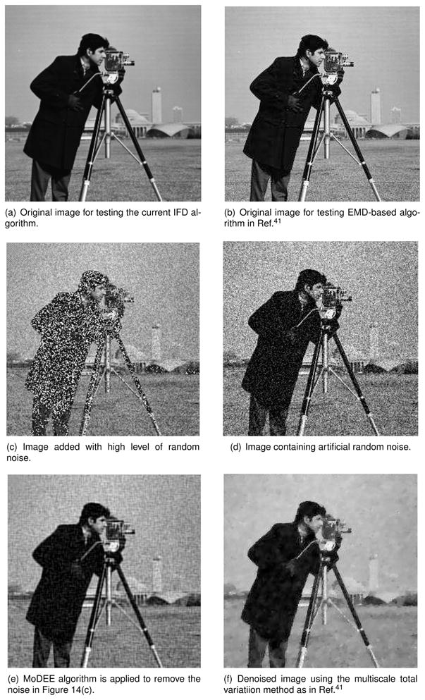
Comparison of IFD with previous EMD algorithms using images with artificial noise. Both algorithms work well. Denoised image in 14(e) conserves better the sharpness of the image, while the one in 14(f) removes background noise more efficiently.

In Figure 15, IFD with just 1 mode is applied to the original image in Figure 15(a). Essentially, it is the direct application of LSEK low pass filter L itself. A small window size of M = 3 is used for edge detection. The image corresponding to mode 1, i.e. I − L, is shown in Figure 15(b).

Figure 15.

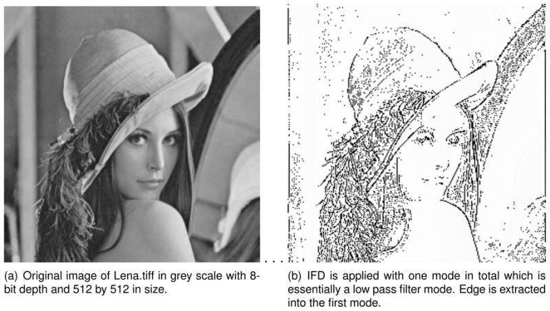
Edge detection using LSEK based IFD.

Now we investigate the smoothing effect when large Gaussian white noise is added in to Figure 15(a). The contaminated image is shown in Figure 16(a). The SNR is measured to be 8dB. The IFD with total 2 modes is applied to the image. In mode 1, a small window size M = 3 is used to remove high-frequency noise, and the residue is shown in Figure 16(b). Then a second mode decomposition follows with larger window size. Due to the flexibility of the LSEK, value of M can be chosen with large flexibility in the range of M ∈ [10, 30]. Mode 2 is thus obtained and subtracted to yield residue of the original image. The whole process is called smoothing. The final image is shown in Figure 16(c). In a similar way as before, we draw a horizontal line in the middle of the image, and plot the values of grey scale along the line. Results are gathered for comparison in Figure 17, in which lines with different color correspond to various modes and residues. The black line corresponds to the original image. The blue and red lines correspond to Figures 16(b) and 16(c). The green line shows the highly oscillatory noise as captured in mode 1. It is clear from the Figure 16 that high and medium levels of oscillatory noises are sequentially captured in modes 1 and 2 using current LSEK based IFD. The resulting images become smooth, but at the cost of edge blurring. All the above results not only show that the IFD with LSEK can be used to effectively smooth noise or detect edge (as in Figure 15), but the IFD modes thus obtained can be effectively and artistically used to reconstruct and enhance the noise-contaminated images.

Figure 16.

Processing image heavily contaminated by Gaussian random noise.

Figure 17.

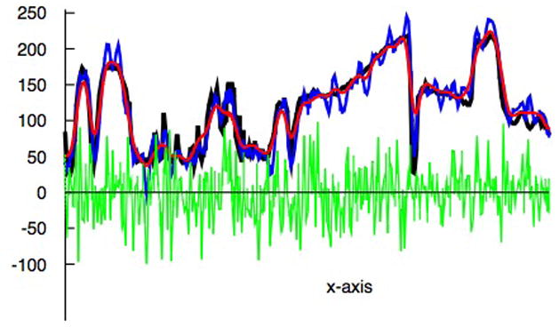
Values of grey scale along the horizontal line across the middle of the corresponding 2D image. Black line shows the values of original image 18(a). Blue lines shows the values for Figure 16(a). Red line shows the values for Figure 16(b). Green line shows the noise captured in the IFD mode.

One unique advantage of the IFD for image and signal processing is the mode reconstruction. Various IMF yielded by the IFD not only reveals the physically important frequencies at various time and length scales, it also provides a way to enhance the image via mode reconstruction, which is for the first time explored in details in this paper. In Figure 18(a), Gaussian white noise is added to the original image in Figure 15(a). Same parameters are used for edge detection as in Figure 15, and this time the first mode shown in Figure 18(b) is contaminated with random noise. Algorithm II.C.3 is applied for image reconstruction. The trend, or partial residue, of mode 1 is shown in Figure 18(c). Note that noise and edge share the similar feature of high frequency oscillation on the same length scale in this case. Since the amplitude of noise is smaller than the one (as shown in Figure 16(d)) added to Figure 16(a), it is more difficult to separate noise from edge. Indeed, as shown in Figure 18(b), one can recognize the edge embedded in the first IFD mode. To enhance the image reconstruction, we continue to apply the IFD (which is termed individual-IFD in Section II.C.3) to extract the trend of mode 1 alone. In Figure 19, we randomly choose one horizontal line (without loss of generality, we choose the horizontal line which cuts the 2D image into halves in the middle) and plot the values of grey scales of this horizontal line. In the figure, z-axis labels the value of grey scale from 0 to 255 in the 8-bit tiff image. The green curve on the bottom of Figure 19 corresponds to the signal contained in mode 1, i.e. noise plus partial edge. The pink curve is obtained as the residue of mode 1, i.e. when individual-IFD is applied to the mode 1. When compared to the black line which shows the values of grey scale for the original non-contaminated image in Figure 15(a), one can clearly tell the similarity between the pink line and black line. It is no doubt that some degree of edge information has been filtered into mode 1 and embedded into the random noise. One then has the choice of adding the residue of mode 1 back into the final results obtained using IFD described above. We call this procedure edge-compensation. Comparison is made between Figures 18(d) and 18(e), where the former is obtained using the standard EMD as before, and the latter is edge-compensated. It is not difficult to visually tell the difference. And signal-to-noise ratio is improved from 20 to 21.7 dB. In Figure 19, blue and red lines correspond to the values of grey scale along the chosen horizontal line for the second IFD mode (i.e. Figure 18(d)) and edge-compensated (i.e. Figure 18(e)) results respectively. When the trend of mode 1 is added back for edge compensation, one can then recover the partial edge mixed with high frequency noise which is filtered after mode 1 extraction. As shown in Figure 18(e), such a compensation leads to visual edge sharpening together with denoising procedure. One can further improve the method by over-compensating edge, i.e. multiply the trend of mode 1 and then add back to the IFD results. This process is essentially edge improvement. In short, with the capability of various IFD modes and strength of the LSEK low pass filter, one can improve the quality and/or analyze the features of images with more flexibility and efficiency.

Figure 18.

Edge restoration/compensation and edge enhancement using edge-noise-decoupling technique based on IFD mode reconstruction.

Figure 19.

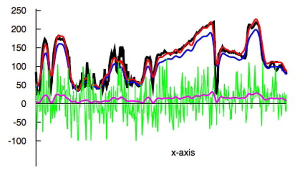
Values of grey scale along the horizontal line across the middle of the corresponding 2D image. Black line shows the values of original image 18(a). Blue lines shows the values for Figure 18(d). Red line shows the values for Figure 18(e). Green line shows the noise captured in IFD mode 1 in Figure 18(b). Pink line shows the values for Figure 18(c).

V Conclusion

A common challenge faced by researchers and decision makers in a wide variety of disciplines as diverse as science, engineering, finance, medicine, and security is the synthesizing information and deriving insight from increasingly massive, dynamic, ambiguous and possibly conflicting data sets. Our objective of collecting and analyzing these data sets is to derive in-depth understanding from them and to facilitate correct decision-making. Conventional analysis tools, such as Fourier analysis, wavelet decomposition, Hilbert transform etc., are insufficient for our current tasks. Recently, iterative filtering decomposition (IFD) has been introduced to address the stability and efficiency issues of the empirical model decomposition (EMD), an emerging powerful method for resolving many challenging problems in data analysis and processing. Another efficient data processing technique is the local spectral evolution kernel (LSEK)⁸¹ which behaves like a perfect low-pass filer with balanced time-frequency localizations. The present work capitalizes the merits of both IFD and LSEK to develop an efficient, flexible, and robust scheme for information extraction, complexity reduction, and signal and image understanding.

The LSEK is combined with the IFD to facilitate an empowered EMD. The theory and algorithm of the proposed LSEK based IFD are presented in detail. The performance of the proposed method is widely validated over a number of common tasks, including mode decomposition, analysis of non-stationary data, information extraction from chaotic data sets, etc. Specific applications are considered to stock market index analysis, ocean wave decomposition, physiologic signal processing and information recovery from noisy images. Some of the best results are obtained in the above mentioned studies. Comparison with earlier methods has also been carried out.

The LSEK based IFD improves the efficiency as well as the stability of the conventional EMD algorithm in applications to a wide category of synthetic, analytic and real time series and images. Specifically, the new algorithm excels in several aspects. First, the LSEK-IFD is capable of extracting more and useful physical features of signals. This is due to the use of the IFD which not only improves the mathematical clarity of the instantaneous frequency characterizing each IFD mode, but also stabilize each mode generation. Secondly, numerical stability and accuracy is enhanced, in part due to the LSEK, a local spectral method, which combines the spectral accuracy of Fourier method and flexibility of local collocation methods. Thirdly, mode reconstruction is proposed for better signal and image analysis and processing. As illustration, it is shown that how one can better reconstruct the image via proper treatment and use of various IFD modes. In particular, it is illustrated that edge can be mixed with equally high frequency noise such that quality of image is reduced in smoothing process. By applying a second individual-IFD to the overall-IFD process, one can extract the edge information embedded in the IFD mode overwhelmed by random noise, and this partial edge information can be used for edge-restoration or edge-enhancement. Therefore, the IFD combined with LSEK can be used to dramatically improve the applicability and performance of the EMD in signal and image processing.

Literature cited

- 1.Aki K, Richards PG. Quantitative seismology. San Francisco, CA: Freeman; 1980. [Google Scholar]
- 2.Anderson JG. Strong motion seismology. Review of GeoPhysics Supplement. 1991;29:700–720. [Google Scholar]
- 3.Archibald R, Gelb A, Saxena R, Xiu DB. Discontinuity detection in multivariate space for stochastic simulations. Journal of Computational Physics. 2009;228:2676–2689. [Google Scholar]
- 4.Archibald R, Gelb A, Yoon Y. Polynomial fitting for edge detection in irregularly sampled signals and images. SIAM Journal on Numerical Analysis. 2005;43:259–279. [Google Scholar]
- 5.Bao G, Wei GW, Zhao S. Local spectral time-domain method for electromagnetic wave propagation. Optics Letters. 2003;28:513–515. doi: 10.1364/ol.28.000513. [DOI] [PubMed] [Google Scholar]
- 6.Bao G, Wei GW, Zhao S. Numerical solution of the Helmholtz equation with high wave numbers. International Journal for Numerical Methods in Engineering. 2004;59:389–408. [Google Scholar]
- 7.Bao W, Sun F, Wei GW. Numerical methods for the generalized Zakharov system. Journal of Computational Physics. 2003;190:201–228. [Google Scholar]
- 8.Bendat JS, Piersol AG. Random data: analysis and measurement procedures. New York: Wiley; 1986. [Google Scholar]
- 9.Benjamin TB, Feir JE. The disintegration of wavetrains on deep water. I. Theory. Journal of Fluid Mechanics. 1967;27:417–430. [Google Scholar]
- 10.Bi N, Sun Q, Huang D, Yang Z, Huang J. Robust Image Watermarking Based on Multiband Wavelets and Empirical Mode Decomposition. Image Processing, IEEE. 2007;16:1956–1966. doi: 10.1109/tip.2007.901206. [DOI] [PubMed] [Google Scholar]
- 11.Boashash B. Estimating and interpreting the instantaneous frequency of a signal. I. Fundamentals. Proceedings of the IEEE. 1992;80:520–538. [Google Scholar]
- 12.Canny J. A computational approach to edge detection. IEEE transactions on pattern analysis and machine intelligence. 1986;8:679–698. [PubMed] [Google Scholar]
- 13.Chan YT. Wavelet basics. Springer; 1995. [Google Scholar]
- 14.Chen K, Chen X, Renaut R, Alexander GE, Bandy D, Guo H, Reiman EM. Characterization of the image-derived carotid artery input function using independent component analysis for the quantitation of [18 F] fluorodeoxyglucose positron emission tomography images. Physics in Medicine and Biology. 2007;52:7055–7071. doi: 10.1088/0031-9155/52/23/019. [DOI] [PubMed] [Google Scholar]
- 15.Chen Q, Huang N, Riemenschneider S, Xu Y. A B-spline approach for empirical mode decompositions. Advances in Computational Mathematics. 2006;24:171–195. [Google Scholar]
- 16.Chen Z, Ivanov PC, Hu K, Stanley HE. Effects of nonstationarities on detrended fluctuation analysis. Physical Review E. 2002;65:041107. doi: 10.1103/PhysRevE.65.041107. [DOI] [PubMed] [Google Scholar]
- 17.Claasen TACM, Mecklenbräuker WFG. The Wigner distributiona tool for time-frequency signal analysis. Part I: Continuous time signals. Philips Journal of Research. 1980;35:372–389. [Google Scholar]
- 18.Cohen L. Time-frequency analysis. Englewood Cliffs, NJ: Prentice-Hall; 1995. [Google Scholar]
- 19.Copson ET. Asymptotic expansions. Cambridge University Press; 1967. [Google Scholar]
- 20.Drazin PG. Nonlinear systems. Cambridge University Press; 1992. [Google Scholar]
- 21.Marr HED. Theory of edge detection. Proceedings of the Royal Society of London: B. 1980;207:187–217. doi: 10.1098/rspb.1980.0020. [DOI] [PubMed] [Google Scholar]
- 22.Echeverría JC, Crowe JA, Woolfson MS, Hayes-Gill BR. Application of empirical mode decomposition to heart rate variability analysis. Medical and Biological Engineering and Computing. 2001;39:471. doi: 10.1007/BF02345370. [DOI] [PubMed] [Google Scholar]
- 23.Equis S, Jacquot P. The empirical mode decomposition: a must-have tool in speckle interferometry? Optics Express. 2009;17:611–623. doi: 10.1364/oe.17.000611. [DOI] [PubMed] [Google Scholar]
- 24.Farge M. Wavelet transforms and their applications to turbulence. Annual Review of Fluid Mechanics. 1992;24:395–457. [Google Scholar]
- 25.Guo H, Renaut RA, Chen K. An input function estimation method for FDG-PET human brain studies. Nuclear medicine and biology. 2007;34:483–492. doi: 10.1016/j.nucmedbio.2007.03.008. [DOI] [PMC free article] [PubMed] [Google Scholar]
- 26.Guo H, Renaut RA, Chen K, Reiman E. FDG-PET parametric imaging by total variation minimization. Computerized Medical Imaging and Graphics. 2009;33:295–303. doi: 10.1016/j.compmedimag.2009.01.005. [DOI] [PMC free article] [PubMed] [Google Scholar]
- 27.Hadley PK, Askar A, Cakmak AS. Subsoil geology and soil amplification in Mexico Valley. Soil Dynamics and Earthquake Engineering. 1991;10:101–109. [Google Scholar]
- 28.Hou ZJ, Wei GW. A new approach for edge detection. Pattern Recogntion. 2002;35:1559–1570. [Google Scholar]
- 29.Hu K, Ivanov PC, Chen Z, Carpena P, Stanley HE. Effects of trends on detrended fluctua-tion analysis. Physical Review E. 2001;64:011114. doi: 10.1103/PhysRevE.64.011114. [DOI] [PubMed] [Google Scholar]
- 30.Huang NE, Long SR, Shen Z. The mechanism for frequency downshift in nonlinear wave evolution. Advances in Applied Mechanics. 1996;32:59–111. [Google Scholar]
- 31.Huang NE, Shen Z, Long SR. A new view of nonlinear water waves: the Hilbert spectrum. Annual Review of Fluid Mechanics. 1999;31:417–457. [Google Scholar]
- 32.Huang NE, Shen Z, Long SR, Wu MC, Shih HH, Zheng Q, Yen N-C, Tung CC, Liu HH. The empirical mode decomposition and the Hilbert spectrum for nonlinear and non-stationary time series analysis. Proceedings of the Royal Society of London: A. 1998;454:903–995. [Google Scholar]
- 33.Huang NE, Tung CC, Long SR. Wave spectra. The Sea. 1990;9:197–237. [Google Scholar]
- 34.Huang NE, Wu Z. A review on Hilbert-Huang transform: Method and its applications to geophysical studies. Reviews of Geophysics. 2008;46:RG2006. [Google Scholar]
- 35.Hwang W, Mallet S. Singularity detection and processing with wavelets. Information Theory, IEEE Transactions on. 1992;38:617–643. [Google Scholar]
- 36.Kevorkian J. Lectures in applied mathematics. Vol. 7. Providence, RI: American Mathematical Society; 1966. Space Mathematics III; pp. 206–275. [Google Scholar]
- 37.Kopsinis Y, McLaughlin S. Development of EMD-based denoising methods inspired by wavelet thresholding. IEEE Transactions on Signal Processing. 2009;57:1351–1362. [Google Scholar]
- 38.Lake BM, Yuan HC. A new model for nonlinear gravity waves. I. Physical model and experimental evidence. Journal of fluid mechanics. 1978;88:33–62. [Google Scholar]
- 39.Li SZ. Markov random field modeling in image analysis. Springer-Verlag; London: 2009. [Google Scholar]
- 40.Liang H, Lin Q-H, Chen JDZ. Application of the Empirical Mode Decomposition to the Analysis of Esophageal Manometric Data in Gastroesophageal Reflux Disease. IEEE Transactions on Biomedical Engineering. 2005;52:1692–1701. doi: 10.1109/TBME.2005.855719. [DOI] [PubMed] [Google Scholar]
- 41.Lin L, Wang Y, Zhou H. Iterative filtering as an alternative algorithm for empirical mode decomposition. Advances in Adaptive Data Analysis. 2009;1:543–560. [Google Scholar]
- 42.Liu B, Riemenschneidera S, Xu Y. Gearbox fault diagnosis using empirical mode decomposition and Hilbert spectrum. Mechanical Systems and Signal Processing. 2006;20:718–734. [Google Scholar]
- 43.Long SR, Huang NE, Tung CC, Wu ML, Lin RQ, Mollo-Christensen E, Yuan Y. The Hilbert techniques: an alternate approach for non-steady time series analysis. IEEE Geoscience Remote Sensing Society Letters. 1995;3:6–11. [Google Scholar]
- 44.Lu Z, Liu Y. Analysis of daily river flow fluctuations using empirical mode decomposition and arbitrary order Hilbert spectral analysis. Journal of Hydrology. 2009;373:103–111. [Google Scholar]
- 45.Mao D, Rockmore DN, Wang Y, Wu Q. EMD Analysis for Visual Stylometry. Preprint. doi: 10.1109/tpami.2012.16. [DOI] [PubMed] [Google Scholar]
- 46.Mao D, Wang Y, Wu Q. A new approach for analyzing physiological time series. Preprint [Google Scholar]
- 47.Miller L, Cheney RE. Large-scale meridional transport in the tropic Pacific Ocean during the 1986–87 El Nino from GEOSAT. Journal of geophysical research. 1990;95:17905–17919. [Google Scholar]
- 48.Miller L, Cheney RE, Douglas BC. GEOSAT altimeter observation of Kelvin waves and the 1986–1987 El Niño. Science. 1988;239:52–54. doi: 10.1126/science.239.4835.52. [DOI] [PubMed] [Google Scholar]
- 49.Newmark NM, Rosenblueth E. Fundamentals of earthquake engineering. Englewood Cliffs, NJ: Prentice-Hall; 1971. [Google Scholar]
- 50.Oppenheim AV, Schafer RW. Digital signal processing. Englewood Cliffs, NJ: Prentice-Hall; 1989. [Google Scholar]
- 51.Pines D, Salvino L. Health monitoring of one dimensional structures using empirical mode decomposition and the Hilbert-Huang Transform. Proceedings of SPIE. 2002;4701:127–143. [Google Scholar]
- 52.Radke RJ, Andra S, Al-Kofahi O, Roysam B. Image change detection algorithms: a systematic survey. IEEE Transactions on Image Processing. 2005;14:294–307. doi: 10.1109/tip.2004.838698. [DOI] [PubMed] [Google Scholar]
- 53.Ramamonjiarisoa A, Mollo-Christensen E. Modulation characteristics of sea surface waves. Journal of geophysical research. 1979;84:7769–7775. [Google Scholar]
- 54.Rezaei D, Taheri F. Experimental validation of a novel structural damage detection method based on empirical mode decomposition. Smart Materials and Structures. 2009;18:045004. [Google Scholar]
- 55.Rilling G, Flandrin P, Gonalves P, Lilly JM. Bivariate empirical mode decomposition. Signal Processing Letters, IEEE. 2007;14:936–939. [Google Scholar]
- 56.Robinson AR, Huang NE, Leitao CD, Parra CG. A study of the variability of ocean currents in the Northwestern Atlantic using satellite altimetry. Journal of physical oceanography. 1983;13:565–585. [Google Scholar]
- 57.Saxena R, Gelb A, Mittelmann H. A high order method for determining the edges in the gradient of a function. Communications of Computational Physics. 2009;5:694–711. [Google Scholar]
- 58.Shao ZH, Wei GW, Zhao S. DSC time-domain solution of Maxwell equations. Journal of computational physics. 2003;189:427–453. [Google Scholar]
- 59.Siddiqi K, Kimia BB, Shu C-W. Geometric shock capturing ENO-schemes for subpixel interpolation, Computation and Curve Evolution. Graphical Models and Image Processing. 1997;59:278–302. [Google Scholar]
- 60.Spedding GR, Browand FK, Huang NE, Long SR. A 2D complex wavelet analysis of an unsteady wind-generated surface wavelet analysis of an unsteady wind-generated surface wave field. Dynamics of atmospheres and oceans. 1993;20:55–77. [Google Scholar]
- 61.Tanaka T, Mandic DP. Complex empirical mode decomposition. Signal Processing Letters, IEEE. 2007;14(101–104) [Google Scholar]
- 62.Tang Y-W, Tai C-C, Su C-C, Chen C-Y, Chen J-F. A correlated empirical mode decomposition method for partial discharge signal denoising. Measurement Science and Technology. 2010;21:085106. [Google Scholar]
- 63.Titchmarsh EC. Introduction to the theory of Fourier integrals. Oxford University Press; 1948. [Google Scholar]
- 64.Vasudevan K, Cook FA. Empirical mode skeletonization of deep crustal seismic data: Theory and applications. Journal of geophysical research. 2000;105:7845–7856. [Google Scholar]
- 65.Wan DC, Patnaik BSV, Wei GW. Discrete singular convolution-finite subdomain method for the solution of incompressible viscous flows. Journal of computational physics. 2002;180:229–255. [Google Scholar]
- 66.Wang Y, Zhou ZF. On the convergence of iterative filtering empirical mode decomposition. Preprint [Google Scholar]
- 67.Wei GW. Discrete singular convolution for the Fokker-Planck equation. Journal of Chemical Physics. 1999;110:8930–8942. [Google Scholar]
- 68.Wei GW. A unified approach for the solution of the Fokker-Planck equation. Journal of Physics A, Mathematics and General. 2000;33:4935–4953. [Google Scholar]
- 69.Wei GW. Discrete singular convolution for the sine-Gordon equation. Physica D. 2000;137:247–259. [Google Scholar]
- 70.Wei GW. A new algorithm for solving some mechanical problems. Computational Methods Applied Mechanics Engineering. 2001;190:2017–2030. [Google Scholar]
- 71.Wei GW, Jia YQ. Synchronization-based image edge detection. EuroPhysics Letters. 2002;59:814–819. [Google Scholar]
- 72.Wei GW, Zhao YB, Xiang Y. Discrete singular convolution and its application to the analysis of plates with internal supports. I. Theory and algorithm. International Journal of Numerical Methods Engineering. 2002;55:913–946. [Google Scholar]
- 73.Whitham GB. Linear and nonlinear waves. New York: Wiley; 1975. [Google Scholar]
- 74.Wu Z, Huang N. Ensemble empirical mode decomposition: A noise-assisted data analysis method. Advances in Adaptive Data Analysis. 2009;1(1):1–41. [Google Scholar]
- 75.Yang P, Wang G, Bian J, Zhou X. The prediction of non-stationary climate series based on empirical mode decomposition. Advances in Atmospheric Sciences. 2010;27:845–854. [Google Scholar]
- 76.Yang SY, Zhou YC, Wei GW. Comparison of the discrete singular convolution algorithm and the Fourier pseudospectral method for solving partial differential equations. Computer Physics Communications. 2002;143:113–135. [Google Scholar]
- 77.Yang W, Tavner P. Empirical mode decomposition, an adaptive approach for interpreting shaft vibratory signals of large rotating machinery. Journal of Sound and Vibration. 2009;321:1144–1170. [Google Scholar]
- 78.Yang Z, Yang L, Qi D, Suen C. An EMD-based recognition method for chinese fonts and styles. Pattern Recognition Letter. 2006;27:1692–1701. [Google Scholar]
- 79.Yeh J-R, Fan S-Z, Shieh J-S. Human heart beat analysis using a modified algorithm of detrended fluctuation analysis based on empirical mode decomposition. Medical Engineering and Physics. 2009;31:92–100. doi: 10.1016/j.medengphy.2008.04.011. [DOI] [PubMed] [Google Scholar]
- 80.Yu S, Zhao S, Wei GW. Local spectral time splitting method for first- and second-order partial differential equations. Journal of Computational Physics. 2005;206(2):727–780. [Google Scholar]
- 81.Yu S, Zhou Y, Wei GW. Matched interface and boundary (MIB) method for elliptic problems with sharp-edged interfaces. Journal of Computational Physics. 2007;224(2):729–756. [Google Scholar]
- 82.Yu Z-G, Anh V, Wang Y, Mao D. Modeling and simulation of the horizontal component of the magnetic field by fractional stochastic differential equations in conjunction with empirical mode decomposition. Journal of Geophysical Research - Space Physics. to appear. [Google Scholar]
- 83.Zhao S, Wei GW. Comparison of the discrete singular convolution and three other numerical schemes for Fishers equation. SIAM Journal of Scientific Computing. 2003;25:127–147. [Google Scholar]
- 84.Zheng Q, Yan XH, Ho CR, Tai CK. The effects of shear flow on propagation of Rossby waves in the equatorial oceans. Journal of physical oceanography. 1994;24:1680–1686. [Google Scholar]
- 85.Zheng Q, Yan XH, Ho CR, Tai CK. Observation of equatorially trapped waves in the Pacific using GEOSAT altimeter data. Deep Sea Research. 1995;42:797–817. [Google Scholar]
- 86.Zhou YC, Patnaik BSV, Wan DC, Wei GW. DSC solution for flow in a staggered double lid driven cavity. International Journal of Numerical Methods and Engineering. 2003;57:211–234. [Google Scholar]
- 87.Zhou YC, Wei GW. High-resolution conjugate filters for the simulation of flows. Journal of Computational Physics. 2003;189:150–179. [Google Scholar]