

Abstract
Several methods for screening gene-environment interaction have recently been proposed that address the issue of using gene-environment independence in a data-adaptive way. In this report, the authors present a comparative simulation study of power and type I error properties of 3 classes of procedures: 1) the standard 1-step case-control method; 2) the case-only method that requires an assumption of gene-environment independence for the underlying population; and 3) a variety of hybrid methods, including empirical-Bayes, 2-step, and model averaging, that aim at gaining power by exploiting the assumption of gene-environment independence and yet can protect against false positives when the independence assumption is violated. These studies suggest that, although the case-only method generally has maximum power, it has the potential to create substantial false positives in large-scale studies even when a small fraction of markers are associated with the exposure under study in the underlying population. All the hybrid methods perform well in protecting against such false positives and yet can retain substantial power advantages over standard case-control tests. The authors conclude that, for future genome-wide scans for gene-environment interactions, major power gain is possible by using alternatives to standard case-control analysis. Whether a case-only type scan or one of the hybrid methods should be used depends on the strength and direction of gene-environment interaction and association, the level of tolerance for false positives, and the nature of replication strategies.
Keywords: case-control studies, efficiency, familywise error rate, genome-wide association study, profile likelihood, robustness, shrinkage
Risks of most complex traits are influenced by both genetic susceptibility and environmental exposures. Epidemiologic researchers have long anticipated that exploration of gene-environment interactions may hold the key to our understanding of the etiology of chronic diseases and that it will ultimately lead to better strategies for disease prevention. In the era of candidate gene studies, studies of gene-environment interactions focused on candidate functional single nucleotide polymorphisms (SNPs), tagging SNPs in candidate genes or in whole candidate pathways that are typically chosen a priori on the basis of hypothesized mechanisms for the effect of the environmental exposure under study. Unfortunately, such hypotheses-driven studies, although conceptually appealing, have not generally been successful in identifying replicable gene-environment interactions. The widely replicated interaction between the N-acetyltransferase 2 gene (NAT2) acetylation activity and smoking on the risk of bladder cancer is a rare exception of success from candidate gene studies (1). Many other claims of interactions, however, have often failed to replicate (2).
Genome-wide association studies (GWAS) now provide tremendous opportunities for large-scale exploration of gene-environment interactions. The agnostic approach of searching for genetic associations based on GWAS has been clearly successful in identifying many susceptibility loci for a wide variety of complex traits (http://www.genome.gov/26525384). However, a large fraction of variation in the different disease phenotypes still remains unknown, with the identified SNPs contributing modestly to prediction of disease risk (3–5). The identified loci are often not within or near genes for which associations could have been expected on an a priori basis. Thus, there is currently hope that an agnostic genome-wide approach may also lead to detection of gene-environment interactions involving previously unsuspected loci (gene-environment wide interaction studies or “GEWIS” as termed by Khoury and Wacholder (6)). Moreover, as GWAS are now being pooled for further discoveries through meta-analysis, various consortia are now beginning to achieve large enough sample sizes necessary for detection of interactions with high confidence. Thomas (7) presents a detailed review, whereas Khoury and Wacholder (6) point out analytical challenges facing large-scale gene-environment (G-E) studies. However, neither of these 2 papers presents numerical results from simulation studies or quantifies the comparative performances of the different methods in terms of metrics related to type I error and power that are relevant to a GWAS.
Population-based case-control studies are commonly used to study the roles of genes and gene-environment interactions in determining the risks of complex diseases. It is well known that standard case-control analysis often has poor power for the detection of multiplicative interaction because of small numbers of cases or controls in cells of crossing genotypes and exposures. In contrast, under the assumption of G-E independence for the underlying population, one can test for multiplicative interaction in a very powerful fashion on the basis of the genotype-exposure correlation in cases alone (8), but the method can have seriously inflated type I error when the underlying assumption of gene-environment independence is violated (9). The independence assumption is quite plausible across the genome for exogenous exposures such as air pollution, pesticides, environmental toxins, or treatment in a randomized clinical trial. The assumption, however, is expected to be violated for some markers in the genome for behavioral exposures, such as smoking and alcohol consumption, or anthropometric traits, such as height and body mass index, which themselves are known to have inherited components.
When the gene-environment association is suspected, practitioners often adopt a 2-stage procedure where, at first, one formally tests for the adequacy of the gene-environment independence assumption on the basis of the data itself and then uses the outcome of that test to decide whether to choose the powerful case-only or the more robust case-control test. For a given study of modest sample size, however, the power of the tests for gene-environment independence would be typically low and, consequently, the 2-stage procedure, as a whole, could still remain significantly biased (9, 10). Use of the independence assumption has been extended to more general analyses that can estimate all the parameters of an association model including main effects and interactions (11, 12). These methods also face the same issue with bias and inflated type I error when genetic and environmental factors are correlated at the population level.
Several authors recently proposed solutions to the bias versus efficiency dilemma by considering hybrid approaches that combine case-control and case-only analysis (13, 14). Murcray et al. (15) proposed a 2-step approach that leverages the independence assumption at an initial screening step. The promising markers are followed up with a standard case-control analysis at the second step. The purpose of this report is to provide a comparative study of these alternative tests for screening gene-environment interactions (G-E effects) with a large number of markers, in terms of type I error and power. Previous results on type I error and power comparison for each of these methods with standard case-control and case-only analyses are separately available in each of the above individual papers, but no comparison across methods is available so far. Cornelis et al. (16) apply several of these methods to analyze G-E interactions in a type 2 diabetes GWAS, but the paper does not contain detailed simulation results. As practitioners are confronting the issue of choosing a method for screening for G-E effects, it is important to realize the advantages and disadvantages associated with each choice. Using simulation studies, in this report, we point out some important operating characteristics of these procedures that could inform/guide such choices.
The report is organized as follows. In the Materials and Methods subsection “Different tests for interaction,” we first describe the different testing procedures that we consider. In the next subsection “Simulation setting,” we describe the simulation design followed to evaluate each method. In the Results section, we present results on type I error and power properties corresponding to these 8 tests under different sampling ratios of cases and controls, different numbers of markers, and varying strength of the G-E association. The Discussion section contains discussion and concluding remarks.
MATERIALS AND METHODS
Different tests for interaction
We present a guiding summary chart of all methods with glossary and key attributes in Table 1. A more detailed description follows below.
Table 1.
Glossary of Methods With Summary Features and Key Attributes
| Method | First Author, Year (Reference No.) | Key Advantages | Key Limitations |
| Case-control | Always maintains type I error rate irrespective of gene-environment association. Robust. Makes no assumption about gene-environment independence/dependence. Can provide tests for joint effects. | Lacks power as a screening tool for discovery of G-E interaction. | |
| Case-only | Piegorsch, 1994 (8) | Valid under G–E independence. Provides substantial gain in terms of power and efficiency under G–E independence. Does not require use of control data and tests association of G and E in cases. Reasonable control of expected number of false positives in large-scale testing even with G–E association being present for a fraction of SNPs. | Severely inflated type I error rates even with a very small fraction of SNPs showing association with environmental exposure. May lose power advantages if the G–E association at the causal locus is negative and the interaction log odds ratio is positive (or vice versa). Cannot yield tests for joint effects and only provides test for interaction. |
| Retrospective profile likelihood-based methods (analogous to CO) | Chatterjee and Carroll (12) | Same as case-only method but can yield estimates of joint effects and subgroup effects by estimating all main effect and interaction parameters under a general likelihood framework. | Inflated type I error rates under departures from the independence assumption. May lose power advantages if the G-E association at the causal locus is negative and the interaction log odds ratio is positive (or vice versa). |
| Empirical BayesEmpirical Bayes, version 2 | Mukherjee, 2008 (13) | A data-adaptive shrinkage approach that provides increase in power compared with CC and superior control of type I error compared with CO. Completely data driven and not reliant on user-defined choices. Works well across all G–E association scenarios. Converges to CC in large sample. EB is preferred over EB2 in terms of MSE. Can test for joint effects. | Does not strictly adhere to nominal type I error level under violation of the G–E independence assumption and moderate sample sizes. Conservative under the independence assumption with lower than nominal type I error levels. Further power improvements can possibly be achieved with more aggressive shrinkage weights. |
| Model averaging Bayesian model averaging Frequentist model averaging (AIC) for G-E studies | Li, 2009 (14) Mukherjee, 2012 (this paper) | Data-adaptive compromise estimators that trade-off between bias and efficiency and combine CC and CO analysis. Similar to the EB approaches in terms of operating characteristics. AIC uses the normalized model AICs as weights and is completely data driven. Works well across all G–E association scenarios. Converges to CC analysis in large samples. Can test joint effects. | Not guaranteed to maintain nominal type I error levels with moderate sample sizes and under violation of G–E independence. Conservative under G–E independence. Bayes model averaging depends on prior weight on the case-control versus case-only analysis, and the results are dependent on this choice. |
| Two-step procedure | Murcray, 2009 (15) | Uses the independence assumption at the first step scan by testing the association of G and E in cases and controls. Filtered markers are followed up by a case-control test. Provides power gain by using a powerful first-step scan and reduction in multiple testing burden at the second step. Always maintains nominal type I error level and provides power gain in most settings. | May lose power advantages when the G–E association is negative and the interaction positive (or vice versa), a situation where case-only also suffers. With more controls than cases, the power advantage over 1-step case-control decreases. The power advantages depend on the choice of the first-step significance threshold. Cannot provide tests for joint effects. |
Abbreviations: AIC, Akaike Information Criterion; CC, case-control; CO, case-only; E, environment; EB, empirical Bayes; EB2, empirical Bayes, version 2; G, gene; MSE, mean-squared error; SNP, single nucleotide polymorphism.
Simple logistic regression based on case-control data.
The simplest and most commonly used test for gene-environment interaction is based on a logistic regression model,
| (1) |
where G = 0, 1, 2 is the number of alleles present at a biallelic locus, E is the environmental exposure, and S are a set of other covariates one may adjust for. We will assume that an ensemble of SNPs have been genotyped for study participants, leading to data on many such genetic factors G. Instead of assuming a trend or log-additive model as the one described above, one can modify the genetic susceptibility model by binary collapsing of G (dominant, recessive) or by allowing separate log odds ratios for each category of G compared with the baseline category, leading to a 2 df test for the main effects of G as well as another 2 df test for the G-E interaction effects. The model for E, when continuous, may involve inclusion of higher-order nonlinear terms. For categorical E, one may again allow separate log odds ratios corresponding to each category of E relative to the baseline category, thus leading to a higher degrees of freedom test for the saturated interaction model. However, we use the simpler notation above with the understanding that appropriate modification of the regression terms can be carried out depending on the nature of G and E. The test for βGE is the standard Wald test for H0: βGE = 0, based on maximum likelihood estimation, or the corresponding likelihood ratio chi-squared test.
Retrospective likelihood-based tests that use gene-environment independence.
Case-only analysis.
In its simplest form, this class of methods includes the popular case-only analysis. This analytical strategy specifies a regression model for testing the association between G and E (conditional on other covariates S) among the cases (D = 1). This can be achieved through modeling the distribution of G|E,S, D = 1 via a polytomous logistic regression model, namely,
| (2) |
Under the assumption of G-E independence conditional on S, the likelihood-ratio test for H0: γ1E = γ2E = 0 among cases in model 2 is a valid test for interaction effects in a corresponding logistic model. More commonly, when a trend model is assumed with a single coefficient γE, such that γ1E = γE and γ2E = 2γE and one employs a Wald test for H0: γE = 0, that test is approximately equivalent to testing H0: βGE = 0 in model 1 with the log-additive assumption.
A major limitation of the case-only analysis, even when the G-E independence assumption is true, is the fact that it cannot yield estimates of the main effect parameters βG and βE that are essential to evaluate the joint effects of G and E, the subgroup effects of a genetic factor across exposure strata, or the effects of an exposure across genotype categories.
Profile likelihood of Chatterjee and Carroll (12).
One can use a log-linear modeling technique for categorical data (11) or a profile likelihood technique more generally (12) and obtain estimates of all model parameters under gene-environment independence using data on both cases and controls. The profile likelihood method has the complete flexibility of a regression model and uses the gene-environment independence assumption (possibly conditional on covariates S that, for example, may include principal components obtained from a large number of genetic markers that can correct for gene-gene and gene-environment dependence that are induced by the presence of population stratification). The method considers a retrospective likelihood,
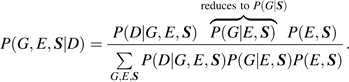 |
(3) |
The ingredients of the above likelihood are specified as below:
A logistic disease incidence model: P(D|G, E, S) of the form from model 1.
A model for P(G|E, S): This is assumed to be of a multinomial logistic form with 3 response categories of G and covariates (E, S). The assumption of G-E independence, conditional on S, implies P(G|E, S) = P(G|S), and the covariate E is simply dropped from this multinomial logit model for P(G|E, S) to reflect the assumption. Let the general G-E dependence model be denoted by
| (4) |
where θgE ≡ 0 and g = 1, 2 under the G-E independence assumption. One can assume a log-additive structure and have one single association parameter θGE as well. The constrained maximum likelihood estimates of the interaction parameters based on this likelihood with θGE ≡ 0 retain the same efficiency advantages as a case-only analysis. One can also incorporate assumptions such as Hardy-Weinberg equilibrium while modeling the distribution of G to further boost the efficiency advantage of a retrospective likelihood (17, 18).
3. A nonparametric model for P(E, S): This renders estimation of a potentially multidimensional nonparametric joint distribution and is handled by the profile likelihood technique established in the report by Chatterjee and Carroll (12). In fact, the likelihood can be treated in an elegant way by establishing equivalence with a simpler pseudo likelihood.
Empirical-Bayes estimation.
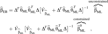
To trade off between bias and the efficiency of case-control and case-only analysis, Mukherjee and Chatterjee (13) proposed a shrinkage estimator based on the above retrospective likelihood framework previously described (12). The estimator is of the following form:
 |
where 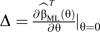 . Here
  denotes estimates of the parameters from model 4, whereas and are parameter estimates and variance estimates obtained from model 3 that allows for gene-environment dependence. Finally, are the constrained maximum likelihood (ML) estimates of the disease-risk parameters from model 3 while using gene-environment independence by setting θgE = 0 in model 4, g = 1, 2. Variance approximations for are provided by Delta approximations in the report by Mukherjee and Chatterjee (13). Wald tests based on approximate asymptotic normality are used. The authors in fact consider another form of shrinkage weight (10) where, in the expression above, is replaced by. The resultant estimator will be denoted by from here onward. The specific form of the “shrinkage” weights is motivated by the expression for the posterior mean obtained in a conjugate analysis under a normal-normal model (19, p. 131), with the prior variance substituted by an estimate obtained using a method of moments approach (20).
The retrospective profile-likelihood methods, including the unconstrained maximum likelihood, constrained maximum likelihood, and empirical Bayes (EB), are now readily implementable in the R-package CGEN (dceg.cancer.gov/bb/tools/genetanalcasecontdata), also available as a part of the R-bioconductor computing repository.
Model averaging.
Bayesian model averaging.
Li and Conti (14) present the following approach that uses case-control data. The method combines the case-only model and the case-control model via the following model-averaging framework, assuming all categorical covariates (G, E).
Note that one can represent the logistic model 1 (without S) by an equivalent log-linear model (M1), where μ represents the cell count of a particular (D, G, E) configuration:
Under the G-E independence assumption, the model above is fitted under constraints that set αGE ≡ 0. Let this reduced model be termed M2. The estimator for βGE under M2 is approximately equivalent to the case-only estimator γ in model 2 for binary G. For a trinary G, under the log-additive trend model, one can assign scores of 0, 1, 2 to the 3 categories of G, which is equivalent to introducing a linear-by-linear association term in the log-linear model for ordinal data (21).
By specifying the prior odds W = P(M1)/P(M2), one can get the posterior distribution of βGE and the resultant Bayes model averaging (BMA) estimator as
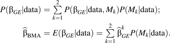 |
The variance expression of the BMA estimator is provided (14), and Wald tests based on the ratio of estimate to standard error are recommended for being used as a test statistic. One can note that the BMA estimator may be computed by using the profile likelihood in model 3 with and without the independence assumption following the same recipe. Using the profile likelihood allows more flexibility than the construct of a log-linear model that limits the analysis to categorical covariates. Li and Conti (14) vary the prior odds-ratio W over a range of values to assess the properties of their method.
Frequentist AIC model averaging.
The notion of combining 2 models is fairly general (22). In addition to the BMA and EB approach, we consider another model-averaged estimator based on the Akaike Information Criterion (AIC). Note that the BMA approach is approximately equivalent to weighting the 2 models by their respective Bayesian Information Criterion (23). In averaging a full model estimate and a reduced model estimate, the EB estimators are also implicitly performing model averaging with a particular choice of model weights (22). One can also use model AICs as alternative weights for the 2 models. For AIC, define w(v) = {1 + exp(v/2 – d)}−1, where d is the dimension of θGE in model 4 or the difference in dimension between the full model (dependence model/unconstrained model) and the reduced model (independence model/constrained model). Let ℒ= 2{ℒdep − ℒindep} be the likelihood ratio test statistic comparing the 2 models. The weight assigned to the reduced (independence) model by AIC is . All models are assumed to be fitted in the profile likelihood framework of Chatterjee and Carroll (12). An approximate variance expression for the AIC averaged estimator is obtained by following an exactly analogous formula to the variance expression in BMA as presented (14), where the Bayesian Information Criterion model weights are replaced by AIC weights.
The 2-step screening strategy.
Murcray et al. (15) proposed a simple but very useful 2-step approach to again leverage the efficiency advantage of case-only type methods for screening, without compromising on the robustness properties of the final tests for gene-environment interaction. Their method can be described through the following steps.
Step 1. A first step screening test: A likelihood ratio test of association between G and E in a combined sample of cases and controls is carried out. For trinary G, test H0: γgE = 0, g = 1, 2 in the following association model:
with γ2E = 2γ1E under a log-additive model.
A subset of m SNPs will exceed a first step threshold of significance α1, with P < α1.
Step 2. For the m SNPs passing through step 1, test H0: βGE = 0 in the logistic model 1. Significance at the second stage is assessed by P < α/m, where α is the overall type I error rate.
The first-step test of the 2-step approach exploits the fact that, under the gene-environment independence assumption in the underlying population, presence of the G-E correlation in the case-enriched case-control sample indicates presence of the gene-environment interaction on the risk of the disease. It is important to note that the first-step test is done in the combined sample of cases and controls and not in cases only. The resulting test is less powerful than a case-only test under gene-environment independence, but the test's being independent of the second-step case-control test ensures that it can be used as a pure “screening” method. Consequently, the 2-step method maintains the nominal type I error level, as the ultimate second-step test is the model-robust case-control test for G-E interaction. The power advantage of the 2-step method comes from reducing the multiplicity burden by decreasing the number of SNPs that are being carried forward to step 2. The amount of power gain of the 2-step procedure depends on the choice of the first-step threshold α1. We use α1 as 0.05 and 5 × 10⁻⁴. Follow-up empirical studies suggest that α1 can be chosen adaptively depending on study size and other parameter guesses for enhanced power.
Remark 1.
Like the case-only approach, one major limitation of the 2-step approach is that one cannot screen for joint effects through this approach, as only the SNPs with significant interaction and not necessarily main effects are carried over to step 2 for the final case-control analysis. Thus, it is very much a targeted interaction searching procedure with the first-step screening test filtering only markers with significant interactions. Moreover, the first-step test statistic is not independent of the second-step test statistic for testing main effects; the independence holds only for testing interaction effects. Thus, for detecting joint effects, this approach is not optimal.
Simulation setting
We first describe the simulation mechanism for any given marker. For the purpose of simulation, we consider the simple setup of an unmatched case-control study with a binary genetic factor G and a binary environmental exposure E. Let E = 1 (E = 0) denote an exposed (unexposed) individual and G = 1 (G = 0) denote whether an individual is a carrier (noncarrier) of the susceptible genotype. Let D denote disease status, where D = 1 (D = 0) stands for an affected (unaffected) individual. Let n0 and n1 be the number of selected controls and cases, respectively. The data can be represented in the form of a 2 × 4 table as displayed in Table 2.
Table 2.
A Binary Genetic Factor and a Binary Environmental Exposure
|
G = 0 |
G = 1 |
|||
| E = 0 | E = 1 | E = 0 | E = 1 | |
| D = 0 | r000 | r001 | r010 | r011 |
| D = 1 | r100 | r101 | r110 | r111 |
Abbreviations: D, disease status; E, environmental exposure; G, genetic factor; r0 and r1, vector of observed cell frequencies in controls and cases, respectively.
Let r0 = (r000, r001, r010, r011) and r1 = (r100, r101, r110, r111) denote the vector of observed cell frequencies in the controls and cases, respectively. The population parameters, namely, the cell probabilities corresponding to a particular G-E configuration in the underlying control and case populations, are denoted as p0 = (p000, p001, p010, p011 = 1 – p000 – p001 – p010) and p1 = (p100, p101, p110, p111 = 1 – p100 – p101 – p110), respectively. The observed vectors of cell counts can be viewed as realizations from 2 independent multinomial distributions, namely, r0 ∼ multinomial (n0, p0) and r1 ∼ multinomial (n1, p1). Let OR10 = p000p101/p001p100 denote the odds ratio associated with E for nonsusceptible subjects (G = 0), OR01 = p000p110/p010p100 denote the odds ratio associated with G for unexposed subjects (E = 0), and OR11 = p000p111/p011p100 denote the odds ratio associated with G = 1 and E = 1 compared with the baseline category G = 0 and E = 0. Therefore,
is the multiplicative interaction parameter of interest. The interaction log odds ratio parameter is βGE = log(ψ).
For each marker, given the values for the prevalence of G and E, namely, PG and PE, and the value of the odds-ratio θGE in the control population, one is able to obtain the control probability vector p0 by solving the following system of equations:
 |
We then set the values of OR10, OR01, and ψ that, together with p0, define the case-probability vector (24). For each marker, we generate data independently from the 2 multinomial distributions corresponding to the case and control populations.
To mimic a large-scale study, we generated data on M markers independently distributed across the genome. For type I error evaluation, we consider the situation with 2,000 cases and 2,000 controls with M = 100,000. For evaluating power characteristics, we consider M = 100,000 with n1 = 2,000, n0 = 2,000 and 4,000, and a larger study with n1 = 10,000, n0 = 10,000 and 15,000. Simulation results for some additional settings with a smaller number of markers M = 10,000 and intermediate sample sizes n1 = 7,000, n0 = 7,000, 14,000 are presented in Web Table 1 (the first of 9 Web tables and 9 Web figures posted on the Journal’s Web site (http://aje.oupjournals.org/)). Throughout, we consider E as a binary environmental covariate with P(E) = 0.5, reflecting a common situation with dichotomization of a continuous covariate at the sample median. All main effect parameters are assumed to be unity, namely, OR10 = OR01 = 1.0 across all scenarios. The trend of results remains unchanged with nonnull main effects.
We assume a situation with only 1 causal locus having true interaction with E and others null with no interaction effect. At the causal locus, the minor allele frequency is set at qA = 0.2, and we assume a dominant genetic susceptibility model with G = 1(AA, Aa), G = 0(aa), yielding P(G = 1) = 0.36. The G-E odds ratio among controls for the causal locus is set at 3 values, namely, exp(θGE) = 1.0, 0.8, 1.1, corresponding to independence, negative, and positive dependence. The interaction parameter at the causal locus exp(βGE) is varied from 1.1 to 2.0 for 2,000 cases and from 1.1 to 1.5 for the situation with 10,000 cases.
Among the M – 1 null loci, without any interaction effects with E, the allele frequency distribution is assumed to be uniform qA ∼ Uniform (0.1, 0.3). The population-level G-E association structure among null loci is assumed to be of the form of a mixture distribution reflecting that a large fraction, e.g., pind, of the SNPs, indeed, is independent of E in the population, whereas the remaining SNPs show some departures from the independence assumption. We generated the log odds ratio of the G-E association in controls corresponding to null loci as Here, δ0 is a point mass at 0 reflecting G-E independence. The standard deviation (sd) parameter of the normal distribution part of the mixture is chosen such that, of the θGE values that depart from independence, 95% fall within ± log(1.5). We vary the simulation parameter pind to create G and E dependence among more (less) null markers.
For the generated ensemble of markers, we then carry out the 8 tests described in Materials and Methods: case-control, case-only, empirical Bayes (EB) and empirical Bayes, version 2 (EB2), 2-step (TS with 2 choices of α1, 0.05 and 5 × 10⁻⁴), BMA (W = 1), and AIC model averaging. In our simulation, we investigate the family-wise type I error rate (FWER), expected number of false positives, and the power of the above testing procedures. All family-wise type I error rates are estimated by the empirical proportion of simulated data sets that declare false significance for H0: βGE = 0 corresponding to at least 1 null marker, using level of significance α/M. We also collect the number of false rejections in each simulation run and present the average of that count over all simulation runs. This estimate of the expected number of false positives may be a more reasonable quantity to examine in a GWAS setting instead of the more conservative FWER that counts the proportion of at least one false rejection. Power values are estimated by the empirical proportion of rejection of H0: βGE = 0 corresponding to the causal marker. The results are based on 5,000 simulated data sets. The margin of error in the estimated proportions with nominal level α = 0.05 with 5,000 simulated data sets is approximately 0.003.
Remark 2.
Under departure from the independence assumption, methods except for the 2-step and the standard case-control analysis may not adhere to strict nominal FWER for all parameter settings considered. We present 2 metrics that combine power and type I error (25) in Web Figures 4–9. The metrics are accuracy (ACC) and positive predictive value (PPV), given by ACC = (1 − type 1 error + power)/2 and PPV = power/(power + type I error). We also present the mean-squared error (MSE) corresponding to each method except the 2-step, which is a pure screening procedure. The MSE provides a combined metric of bias and variance from an estimation standpoint.
RESULTS
We now summarize the main findings of the simulation study. Table 3 presents the FWER and expected number of false positives corresponding to each method with M = 100,000 for various values of pind from 0.95 to 1.00, the proportion of markers that follow gene-environment independence. The simulation is carried out with n1 = n0 = 2,000. One can note that the 2-step and the case-control procedures always maintain FWER, whereas the FWER for the case-only method is at 0.80 even when 99.95% of the SNPs are independent of E. The FWER control of EB-type procedures and model-averaging procedures is much superior than the case-only method, and FWER is maintained if the fraction of SNPs that actually follow the G-E independence assumption is 99.0% or more. The model-averaging procedures BMA and AIC offer better control of FWER compared with EB-type procedures when pind is lower, for example, 0.95, when more than 5% of SNPs are associated with E. One may note that, for higher values of pind closer to 1.00, which is likely to be realistic in practice, the EB-type as well as model-averaging procedures can maintain strict FWER and even be conservative. Web Table 1 contains FWER results with M = 10, 000.
Table 3.
Family-Wise Type I Error Rate (Expected Number of False Positives) Corresponding to the 8 Testing Procedures When pind Varies From 0.95 to 1.00a,b
| pind | Method |
|||||||
| CC | CO | EB | EB2 | TS (α1 = 0.0005) | TS (α1 = 0.05) | AIC | BMA | |
| 0.9500 | 0.050 (0.051) | 1.000 (158.444) | 0.186 (0.205) | 0.138 (0.148) | 0.058 (0.059) | 0.048 (0.048) | 0.064 (0.065) | 0.068 (0.068) |
| 0.9900 | 0.047 (0.047) | 1.000 (30.795) | 0.057 (0.058) | 0.042 (0.043) | 0.051 (0.051) | 0.037 (0.038) | 0.033 (0.034) | 0.033 (0.034) |
| 0.9950 | 0.050 (0.051) | 1.000 (14.772) | 0.036 (0.036) | 0.031 (0.032) | 0.054 (0.056) | 0.049 (0.050) | 0.031 (0.032) | 0.032 (0.033) |
| 0.9975 | 0.046 (0.047) | 1.000 (7.038) | 0.026 (0.036) | 0.025 (0.025) | 0.052 (0.053) | 0.050 (0.052) | 0.033 (0.033) | 0.029 (0.030) |
| 0.9995 | 0.046 (0.048) | 0.802 (0.830) | 0.022 (0.023) | 0.022 (0.023) | 0.047 (0.049) | 0.048 (0.050) | 0.030 (0.031) | 0.030 (0.031) |
| 1.0000 | 0.047 (0.049) | 0.041 (0.042) | 0.016 (0.016) | 0.016 (0.017) | 0.047 (0.048) | 0.043 (0.044) | 0.030 (0.030) | 0.031 (0.031) |
Abbreviations: AIC, Akaike Information Criterion; BMA, Bayesian model averaging; CC, case-control; CO, case-only; EB, empirical Bayes; EB2, empirical Bayes, version 2; pind, probability of a single nucleotide polymorphism independent of environmental exposure; SNP, single nucleotide polymorphism; TS, 2 step.
The number of markers considered is 100,000 (M = 100,000).
The simulated 5,000 replicate data sets included 2,000 cases and 2,000 controls, each with genotype information on M = 100,000. This ensures simulation accuracy for type I error rates of the order of 0.003 at α1 = 0.05. The prevalence of exposure (E) is 0.5, and the allele frequency of genotype (G) at the causal locus is 0.2; allele frequencies among null markers are uniformly distributed as [0.1, 0.3]. The odds ratios for E (OR10) and G (OR01) at all loci are fixed at 1.0, and the interaction effect size (exp(βGE)) at the causal locus is fixed at the null value 1.00. The probability of a null SNP independent of E, pind, varies from 0.95 to 1.0. The family-wise type I error rate is estimated as the empirical proportion of data sets declaring at least 1 null marker to be significant. The expected number of false positives is estimated as the average number of falsely rejected null hypotheses, averaged over 5,000 data sets.
In terms of the expected number of false positives in Table 3, the case-only analysis is still worse among all methods but does not appear to be an unreasonable strategy with the expected number of false positives less than 1 when pind = 0.9995 and around 7 when pind = 0.9975, which rises to around 158 with pind = 0.95. This may be a more rational metric to examine in GWAS instead of FWER, which considers only the more conservative criterion of probability of at least 1 false rejection under the global null hypotheses.
Figures 1 and 2 represent the power values for testing H0: βGE = 0 at the causal locus for the 8 methods with M = 100,000. The exact numerical values corresponding to the graphs are contained in the Web tables and figures. The fraction of null SNPs that satisfy the independence assumption is set at 0.995 in each case.
Figure 1.

Empirical power curves for the 8 approaches: case-control (CC), case-only (CO), empirical Bayes (EB) and empirical Bayes, version 2 (EB2), 2 step (TS) with different first step α1, Akaike Information Criterion (AIC) model averaging, and Bayes model averaging (BMA with weights W = 1). Genotype information is generated on M = 100,000 markers. The interaction effect size (exp(βGE)) at the causal locus varies from 1.0 to 2.0. The top panel corresponds to 2,000 cases and 2,000 controls, whereas the bottom panel corresponds to 2,000 cases and 4,000 controls. The left, center, and right panels correspond to different values of the G-E odds ratio at the causal locus, namely, exp(θGE) = 0.8, 1.0, and 1.1, respectively. The prevalence of exposure (E) is 0.5, and the allele frequency of genotype (G) at the causal locus qA is set at 0.2. For null loci, the allele frequencies are uniformly distributed on [0.1, 0.3]. The percentage of null loci that are independent of E is fixed at pind = 0.995. The marginal odds ratios for E (OR10) and G (OR01) are fixed at 1.00 for all loci. Results are based on 5,000 simulated data sets.
Figure 2.

Empirical power curves for the 8 approaches: case-control (CC), case-only (CO), empirical Bayes (EB) and empirical Bayes, version 2 (EB2), 2 step (TS) with different first step α1, Akaike Information Criterion (AIC) model averaging, and Bayes model averaging (BMA with weights W = 1). Genotype information is generated on M = 100,000 markers. The interaction effect size (exp(βGE)) at the causal locus varies from 1.0 to 1.5. The left, center, and right panels correspond to different values of the G-E odds ratio at the causal locus, namely, exp(θGE) = 0.8, 1.0, and 1.1, respectively. The top panel corresponds to 10,000 cases and 10,000 controls, whereas the bottom panel corresponds to 10,000 cases and 15,000 controls. The prevalence of exposure (E) is 0.5, and the allele frequency of genotype (G) at the causal locus qA is set at 0.2. For null loci, the allele frequencies are uniformly distributed on [0.1, 0.3]. The percentage of null loci that are independent of E is fixed at pind = 0.995. The marginal odds ratios for E (OR10) and G (OR01) are fixed at 1.00 for all loci. Results are based on 5,000 simulated data sets.
We first discuss the main features in Figure 1 with n1 = n0 = 2,000 when the independence assumption holds at the causal locus (exp(θGE) = 1.0). As expected, case-only analysis has the maximum power compared with all other contenders. Among hybrid methods, the 2-step and EB perform similarly, and these 2 methods generally have higher power than BMA or AIC. The 2-step approach with α1 = 5 × 10⁻⁴ has slightly higher power than EB for an interaction odds ratio exceeding 1.6. For example, with n1 = n0 = 2,000, at interaction odds ratio = 1.8, the power of EB is 0.68, of EB2 is 0.58, and of BMA and AIC is 0.59, whereas the 2-step method with α1 = 5 × 10⁻⁴ has power of 0.74. In this setting, the 2-step method with α1 = 0.05 attains a power of 0.53. The case-only method has power of 0.92, whereas the case-control analysis has a low power of 0.31. For lower values of the interaction odds ratio (≤1.6), the EB and TS have very similar performance, and they outperform the model-averaging approaches. For example, at interaction odds ratio = 1.6, both EB and TS (α1 = 5 × 10⁻⁴) have a power of 0.30, whereas the power of BMA and AIC is 0.18. The EB2 power is at 0.23, whereas TS with α1 = 0.05 has power of 0.20. The case-control and case-only analyses have power values of 0.08 and 0.54, respectively. For an interaction odds ratio less than 1.3, the EB procedure appeared to have slightly greater power than TS, but both of the power values were very low under this sample size.
The bottom panel of Figure 1 with n1 = 2,000 and n0 = 4,000 shows a similar trend but weaker performance by the TS method with both choices of α1. With the case:control ratio being tilted toward having more controls than cases, the first-step screening test in the combined sample of cases and controls loses the power advantage of a case-only approach when compared to 1:1 case:control ratio. Thus, we note a surprising and counterintuitive finding that, under identical simulation settings, the power of the 2-step procedure actually decreases with an increasing number of controls, if the number of cases is held fixed, as the power depends on the case:control ratio. For example, under the independence assumption, with interaction odds ratio = 1.9, with n0 = 2,000, TS (α1 = 5 × 10⁻⁴) has power of 0.87 that reduces to 0.82 as n0 increases to 4,000. On the other hand, under the same setting, the power of TS (α1 = 0.05) is 0.69 with n0 = 2,000 and increases to 0.89 with n0 = 4,000. This indicates that the optimal screening threshold α1 in the 2-step procedure does heavily depend on the case:control ratio, everything else remaining the same.
Under departures from the independence assumption at the causal locus, we consider 2 situations: one with a positive and the other with a negative association between G and E in the controls. With (exp(θGE) = 1.1), again the case-only method has the highest power, and the 2-step with α1 = 5 × 10⁻⁴ has the second highest power and a clear dominance over other hybrid methods. In contrast, under negative dependence at the causal locus (exp(θGE) = 0.8), case-control analysis is the most powerful analysis, and case-only analysis performs quite poorly (refer also to the report by Li and Conti (14)). In this situation, where βGE is positive and θGE is negative, the G-E log odds ratio in cases (which is simply βGE + θGE for a 2 × 4 table) is close to null, explaining the loss of power. The 2-step approach also performs quite poorly in this setting, especially with the more stringent choice of α1 = 5 × 10⁻⁴. The BMA, EB, EB2, and AIC perform comparably among the hybrid methods, with BMA/AIC having an edge over the EB-type methods in this scenario. The loss of power in TS under a study design with more controls than cases becomes quite drastic with negative G-E association as one can notice in the leftmost panels of Figure 1. TS with both choices of α1 loses power as n0 increases under such negative dependence.
In order to understand the phenomenon of the better power property of EB over TS at smaller values of interaction odds ratio under independence, we increased the sample size to n1 = 10,000 and repeated the same simulation over a more modest range of interaction odds ratio from 1.1 to 1.5. Figure 2 essentially captures the same features of the different methods as discussed for Figure 1. Under independence, EB has power advantages over TS for smaller values of interaction, especially for an unequal case:control ratio (bottom panel, center graph, in Figure 2). Under positive dependence, TS has a clear dominance and, under negative dependence, BMA/AIC has the advantage over EB, whereas TS performs quite poorly. This larger sample size setting is more reflective of current post-GWAS consortium studies exploring G-E effects. Results for several other simulation settings are presented in Web Figures 1–3. Exact numbers corresponding to each figure are contained in Web Tables 2–9.
Figure 3 presents the estimated relative MSE corresponding to the log odds-ratio parameter at the causal locus under the simulation setting of Figure 1 for all the methods except the 2-step method (which is more of a screening tool and not an estimation method). The MSE for each method is divided by the MSE of standard case-control analysis. One can notice the advantage of EB-type methods in terms of this metric as one tries to balance between bias and efficiency in a data-adaptive way. The case-only method is best only when the independence assumption is true (the central block) and performs worse under any departures from the independence assumption.
Figure 3.

Relative mean-squared error of the 6 approaches except for the 2-step approach corresponding to the estimation of βGE at the causal locus. The 6 approaches are case-control (CC), case-only (CO), empirical Bayes (EB) and empirical Bayes, version 2 (EB2), Akaike Information Criterion (AIC) model averaging, and Bayes model averaging (BMA with weights W = 1). All mean-squared errors are divided by the corresponding mean-squared error of the standard case-control analysis. The interaction effect size (exp(βGE)) at the causal locus varies from 1.0 to 2.0. The top panel corresponds to 2,000 cases and 2,000 controls, whereas the bottom panel corresponds to 2,000 cases and 4,000 controls. The left, center, and right panels correspond to different values of the G-E odds ratio at the causal locus, namely, exp(θGE) = 0.8, 1.0, and 1.1, respectively. The prevalence of exposure (E) is 0.5, and the allele frequency of genotype (G) at the causal locus qA is set at 0.2. Results are based on 5,000 simulated data sets.
DISCUSSION
In summary, our study indicates that the data-adaptive hybrid methods EB, TS, BMA, or AIC model averaging can achieve balance between power gain and type 1 error rate control for testing G-E effects in large-scale association studies. There is no uniform dominance of one method versus the other in terms of their operating characteristics across all simulation scenarios. The performance of the methods differs according to magnitude/direction of the G-E association and interaction odds ratio. All the new hybrid methods offer power gain over standard case-control analysis and better control of type I error rate compared with a case-only analysis. We summarize and conclude with some observations that merit further discussion.
Type I error control
We note that, even if only a very small fraction of the SNPs actually departs from independence, for example, 0.05% (pind = 0.9995 in Table 1), using a case-only method will still not offer nearly adequate control of type I error rates to prioritize lead G-E candidates, whereas the hybrid approaches offer protection from false positives. An attractive feature of the 2-step method is that it always maintains the desired level of FWER. The EB-type methods have worse FWER control compared with model averaging when the fraction of SNPs truly associated with E is more than 1% (under the G-E association distribution we assumed among the null markers). However, in a GWAS study, to expect the fraction of SNPs departing from independence assumption to be much less than 1% may be a quite realistic assumption and, in that range of pind, all the weighted methods maintain nominal FWER. We note that, if the prior probability for the case-only model is increased in BMA, it boosts the power but inflates the FWER as one would expect. However, one can always postulate alternative distributions for G-E association parameters among the null loci, instead of the mixture distribution we assumed, and the operating characteristics of the methods in terms of FWER will change substantially on the basis of that distribution. Note that, for the small fraction of markers that departs from independence, we assumed a N(0, sd = log(1.5)/2) distribution. Further shrinking the variance of this distribution leads to an improvement in the FWER properties of case-only and all hybrid methods.
Another interesting observation is the fact that, for pind exceeding 0.99, the weighted methods have a conservative FWER, falling well below 0.05. Thus, there is some scope of using a more aggressive form of shrinkage and enhancing the power of these methods further.
We observe that, if one desires to control the number of false positives instead of FWER, a case-only analysis appears to perform quite reasonably in a range of scenarios for gene-environment association that is likely to arise in practice (pind between 0.995 and 1.00). If, in a GWAS, discoveries are going to be followed by replication, it may be reasonable to accept a few false positives if a significant boost in power occurs by using a specific method. Still, caution is needed to avoid a large number of false positives, as they could infiltrate the limited number of top-ranked SNPs that may be followed up for replication.
Power comparison
In general, under the independence assumption and for positive G-E association, the case-only method has the highest power. The 2-step approach is preferred over the case-only approach for positive association scenarios, as it maintains FWER, which the case-only method does not. The power properties of the methods when the G-E interaction is positive and the G-E association is negative are worth noting, as this may very likely occur for a fraction of SNPs in a large-scale association study. Case-only analysis is not the most powerful analysis in such situations, and a standard case-control analysis can be more powerful. The weighted methods strike a compromise in this reverse situation as well. The performance of the 2-step method in such situations is concerning, as it suffers severely from the lack of power of the first-step case-only type screening procedure, especially with a more stringent choice of the first-step threshold α1.
The power performance of the 2-step method in terms of study designs where the control:case ratio is larger than 1:1 is also noteworthy and has not been previously pointed out. The first-step screening test for interaction in the 2-step method can be viewed as a weighted test of G-E association in cases and in controls. When the weight corresponding to controls increases, there is an attenuation of the test statistic, leading to a loss of power. In fact, because of such phenomena, there could be situations where the power of the 2-step method, as a whole, may decrease, as the number of controls is increased, everything else remaining fixed. The power loss of the 2-step method is more pronounced for negative G-E association in controls and positive interaction (or vice versa). In this situation, very few of the “promising” SNPs filter through the screening step causing this behavior. One may attempt to correct this drawback by attaching differential sampling weights to case and control observations in the first-step screening procedure, but that will destroy the desirable independence property of the first-step screening test with the second-step case-control test.
Given the sample-size and G-E association configurations, it appears that the weighted methods EB, EB2, BMA, and AIC have the robustness advantage of performing reasonably well across a spectrum of alternatives in terms of their power properties. Among the weighted methods, EB has advantage over BMA/AIC in the situation with a positive G-E association, whereas BMA has power advantage in the negative G-E association scenario.
Combined metrics of power and type 1 error
Because 5 of the 7 methods may not adhere to nominal type I error levels (in the sense of FWER), in Web Figures 4–9 we present 2 combined metrics ACC and PPV as described before. One can notice that the case-only method is least desirable in terms of these metrics even when pind = 0.9995. The performance of the hybrid methods across a spectrum of G-E association scenarios is indeed encouraging.
Estimation and testing for effects other than multiplicative interaction
In this article, we have focused on tests for multiplicative interactions only. It is, however, important to recognize that the value of studying genetic and environmental exposures together does not necessarily stem from the ability to test for statistical interactions. Various alternative parameters, such as the joint effect of 2 exposures or the subgroup effects of 1 exposure within strata defined by the other exposure, may be useful for developing powerful tests of association, understanding the public health impact of the exposures, targeting intervention, and risk prediction. The hybrid procedures can be extended to carry out inference regarding such alternative parameters of interest. In recent years, for example, omnibus tests, which can simultaneously account for genetic main effects and gene-environment/gene-gene interactions, have received attention as a powerful approach for the detection of disease susceptibility loci (26, 27). A major limitation of the 2-step method is that it is targeted toward testing for only multiplicative interactions and cannot be easily generalized to alternative tests that may involve main-effect parameters (refer to “Remark 1”).
Sensitivity to user-defined choices
The choice of the first-step threshold α1 can largely determine the power properties of the 2-step approach. It is hard to optimize this choice for a large-scale study as it depends on the number of markers, disease prevalence, case:control ratio, distribution of unknown G-E association parameters, and interaction effect sizes. In a more recent article, an optimal choice of α1 has been proposed (28), and α1 = 0.0005 that we have used is found to be nearly optimal under most of our simulation configurations. The performance of the BMA procedure can also change by varying the ratio of prior weights W. We used W = 1 in our study, but it may be more reasonable to assign a larger prior mass to the case-only model or to the assumption of gene-environment independence. On the other hand, the EB procedures and AIC averaging do not require any prior or tuning parameter specification and are completely data adaptive.
Analytical power calculation is intractable in closed form for the hybrid methods, and we resort to simulation studies to evaluate the current ensemble of methods. We have presented results under 1 particular simulation scheme, and the trend in the results remains similar for changes in simulation parameters such as the allele frequency, exposure prevalence, number of cases and controls with a given case:control ratio, and number of markers. However, if one changes the parameters of the mixture distribution for or uses an alternate form of distribution as elicited by Park et al. (5), the FWER comparison may change appreciably.
Issues with lack of coherence and violation of the likelihood principle
A reviewer has raised an important point that some of these methods (case-only, 2-step) ignore data and still gain power. This may appear to be counterintuitive to foundational statistical principles and raises the question, “How can ignoring data lead to better performances than using the entire information content of a data set?” The case-only approach makes a strong assumption to gain efficiency and provides unbiased estimates only under the assumption of gene-environment independence. However, the method is “coherent” in the sense that it can be justified via a proper “likelihood” of the entire data as long as the independence assumption is valid (11, 12). Note in Figures 1 and 2 (central block) that, when the independence assumption is true, the case-only method that yields the constrained MLE is indeed optimal in terms of power. However, as our simulation study has shown, the gain in power by making this assumption comes at a price of inflated FWER, under departures from this assumption. If instead of controlling the FWER, one is willing to accept a limited number of false positives, the case-only type approach may be a reasonable strategy, if we believe that only a handful of SNPs in a GWAS may be truly associated with the environmental exposure under consideration (the situations corresponding to pind ≥ 0.9975 in Table 3).
In contrast, the 2-step method essentially divides information in the total likelihood into 2 independent components, one used for screening and the other for validation. In general, these types of 2-step screening strategies that partition the total information in the data set for a clever work-around of the multiple testing problem cannot be justified on the basis of a likelihood principle and, thus, sometimes can face “incoherence” issues. For example, we have noted earlier that, in some situations, the power of the 2-step method may decrease as the sample size for controls increase in a study, everything else remaining fixed. Future researchers are encouraged to explore methods that can combine the 2 independent sources of information used in the 2-step procedure in a more coherent fashion, while retaining the desirable unbiased property that the type I error rate for the procedure overall is not influenced by the underlying gene-environment independence assumption. Analogous developments have recently taken place for combining within- and between-family information in family-based association studies (29).
The current study is certainly not exhaustive. For example, Kooperberg and Leblanc (30) proposed another 2-step approach to screen for G-G effects by filtering the marginal genetic associations and restricting interaction testing to this subset. Similar strategies can be adapted to G-E screening. Murcray et al. (28) propose a hybrid approach that combines the above Kooperberg-Leblanc marginal screening and the 2-step screening of Murcray et al. (15) to improve upon the original 2-step procedure. The new paper (28) addresses some of the critiques pointed out in the discussion of the original paper by Chatterjee and Wacholder (31), specifically the issue of choosing the optimal α1. These new and improved methods may be included in the future to expand on the findings of the current study. We primarily considered case-control sampling and did not consider family-based designs. Gauderman et al. (32) extended the 2-step method for G-E interactions in case-parent trios. It remains an interesting open question to compare the hybrid methods under studies that include related individuals.
To conclude, we find it encouraging that, under realistic violations of gene-environment independence, the hybrid procedures can protect against false positives due to gene-environment association and yet can gain substantial power over the standard case-control analysis. Moreover, under a range of realistic scenarios, the hybrid methods are likely to be conservative, and further power gain is possible by using case-only type methods, assuming that a moderate number of false positives could be ruled out in further replication studies. Thus, future analyses of gene-environment interactions in GWAS are likely to benefit by using the new alternatives.
Software
The R codes for simulating power for the different tests of interaction are available from the corresponding author upon request. The R-package CGEN for semiparametric maximum likelihood and the EB procedure is available at http://dceg.cancer.gov/bb/tools/genetanalcasecontdata.
Supplementary Material
Acknowledgments
Author affiliations: Department of Biostatistics, School of Public Health, the University of Michigan, Ann Arbor, Michigan (Bhramar Mukherjee, Jaeil Ahn); Department of Internal Medicine, Human Genetics, and Epidemiology, the University of Michigan, Ann Arbor, Michigan (Stephen B. Gruber); and Division of Cancer Epidemiology and Genetics, National Cancer Institute, National Institutes of Health, Rockville, Maryland (Nilanjan Chatterjee).
This research was partially supported by National Institutes of Health grant CA-156608 and National Science Foundation grant DMS-1007494 to B. M., National Institutes of Health grant U19 NCI-895700 to S. B. G. and B. M., and the Intramural Research Program of the National Cancer Institute to N. C.
The authors thank Duncan Thomas and others for their valuable suggestions that strengthened the manuscript. The authors are grateful to David V. Conti and Dailin Li for sharing their R codes for the BMA method.
Conflict of interest: none declared.
Glossary
Abbreviations
- ACC
accuracy
- AIC
Akaike Information Criterion
- BMA
Bayes model averaging
- EB
empirical Bayes
- EB2
empirical Bayes, version 2
- FWER
family-wise type I error rate
- G-E
gene-environment
- GWAS
genome-wide association study(ies)
- MSE
mean-squared error
- PPV
positive predictive value
- SNP
single nucleotide polymorphism
- TS
2 step
References
- 1.García-Closas M, Malats N, Silverman D, et al. NAT2 slow acetylation, GSTM1 null genotype, and risk of bladder cancer: results from the Spanish Bladder Cancer Study and meta-analyses. Lancet. 2005;366(9486):649–659. doi: 10.1016/S0140-6736(05)67137-1. [DOI] [PMC free article] [PubMed] [Google Scholar]
- 2.Risch N, Herrell R, Lehner T, et al. Interaction between the serotonin transporter gene (5-HTTLPR), stressful life events, and risk of depression: a meta-analysis. JAMA. 2009;301(23):2462–2471. doi: 10.1001/jama.2009.878. [DOI] [PMC free article] [PubMed] [Google Scholar]
- 3.Gail MH. Discriminatory accuracy from single-nucleotide polymorphisms in models to predict breast cancer risk. J Natl Cancer Inst. 2008;100(14):1037–1041. doi: 10.1093/jnci/djn180. [DOI] [PMC free article] [PubMed] [Google Scholar]
- 4.Wacholder S, Hartge P, Prentice R, et al. Performance of common genetic variants in breast-cancer risk models. N Engl J Med. 2010;362(11):986–993. doi: 10.1056/NEJMoa0907727. [DOI] [PMC free article] [PubMed] [Google Scholar]
- 5.Park JH, Wacholder S, Gail MH, et al. Estimation of effect size distribution from genome-wide association studies and implications for future discoveries. Nat Genet. 2010;42(7):570–575. doi: 10.1038/ng.610. [DOI] [PMC free article] [PubMed] [Google Scholar]
- 6.Khoury MJ, Wacholder S. Invited commentary: from genome-wide association studies to gene-environment-wide interaction studies—challenges and opportunities. Am J Epidemiol. 2009;169(2):227–230. doi: 10.1093/aje/kwn351. [DOI] [PMC free article] [PubMed] [Google Scholar]
- 7.Thomas D. Gene–environment-wide association studies: emerging approaches. Nat Rev Genet. 2010;11(4):259–272. doi: 10.1038/nrg2764. [DOI] [PMC free article] [PubMed] [Google Scholar]
- 8.Piegorsch WW, Weinberg CR, Taylor JA. Non-hierarchical logistic models and case-only designs for assessing susceptibility in population-based case-control studies. Stat Med. 1994;13(2):153–162. doi: 10.1002/sim.4780130206. [DOI] [PubMed] [Google Scholar]
- 9.Albert PS, Ratnasinghe D, Tangrea J, et al. Limitations of the case-only design for identifying gene-environment interactions. Am J Epidemiol. 2001;154(8):687–693. doi: 10.1093/aje/154.8.687. [DOI] [PubMed] [Google Scholar]
- 10.Mukherjee B, Ahn J, Gruber SB, et al. Tests for gene-environment interaction from case-control data: a novel study of type I error, power and designs. Genet Epidemiol. 2008;32(7):615–626. doi: 10.1002/gepi.20337. [DOI] [PubMed] [Google Scholar]
- 11.Umbach DM, Weinberg CR. Designing and analysing case-control studies to exploit independence of genotype and exposure. Stat Med. 1997;16(15):1731–1743. doi: 10.1002/(sici)1097-0258(19970815)16:15<1731::aid-sim595>3.0.co;2-s. [DOI] [PubMed] [Google Scholar]
- 12.Chatterjee N, Carroll RJ. Semiparametric maximum likelihood estimation exploiting gene-environment independence in case-control studies. Biometrika. 2005;92:399–418. [Google Scholar]
- 13.Mukherjee B, Chatterjee N. Exploiting gene-environment independence for analysis of case-control studies: an empirical Bayes-type shrinkage estimator to trade-off between bias and efficiency. Biometrics. 2008;64(3):685–694. doi: 10.1111/j.1541-0420.2007.00953.x. [DOI] [PubMed] [Google Scholar]
- 14.Li D, Conti DV. Detecting gene-environment interactions using a combined case-only and case-control approach. Am J Epidemiol. 2009;169(4):497–504. doi: 10.1093/aje/kwn339. [DOI] [PMC free article] [PubMed] [Google Scholar]
- 15.Murcray CE, Lewinger JP, Gauderman WJ. Gene-environment interaction in genome-wide association studies. Am J Epidemiol. 2009;169(2):219–226. doi: 10.1093/aje/kwn353. [DOI] [PMC free article] [PubMed] [Google Scholar]
- 16.Cornelis MC, Tchetgen Tchetgen EJ, Liang L, et al. Gene-environment interactions in genome-wide association studies: a comparative study of tests applied to empirical studies of type 2 diabetes. Am J Epidemiol. 2012;175(3):191–202. doi: 10.1093/aje/kwr368. [DOI] [PMC free article] [PubMed] [Google Scholar]
- 17.Chen J, Chatterjee N. Exploiting Hardy-Weinberg equilibrium for efficient screening of single SNP associations from case-control studies. Hum Hered. 2007;63(3-4):196–204. doi: 10.1159/000099996. [DOI] [PubMed] [Google Scholar]
- 18.Luo S, Mukherjee B, Chen J, et al. Shrinkage estimation for robust and efficient screening of single-SNP association from case-control genome-wide association studies. Genet Epidemiol. 2009;33(8):740–750. doi: 10.1002/gepi.20428. [DOI] [PMC free article] [PubMed] [Google Scholar]
- 19.Berger JO. Statistical Decision Theory and Bayesian Analysis. New York, NY: Springer Verlag; 1985. [Google Scholar]
- 20.Greenland S. Methods for epidemiologic analyses of multiple exposures: a review and comparative study of maximum-likelihood, preliminary-testing, and empirical-Bayes regression. Stat Med. 1993;12(8):717–736. doi: 10.1002/sim.4780120802. [DOI] [PubMed] [Google Scholar]
- 21.Agresti A. Categorical Data Analysis. 2nd ed. New York, NY: John Wiley and Sons; 2002. [Google Scholar]
- 22.Hjort NL, Claeskens G. Frequentist model average estimators (with discussion) J Am Stat Assoc. 2003;98(464):879–899. [Google Scholar]
- 23.Schwarz G. Estimating the dimension of a model. Ann Stat. 1978;6(2):461–464. [Google Scholar]
- 24.Satten GA, Kupper LL. Inferences about exposure-disease associations using probability-of-exposure information. J Am Stat Assoc. 1993;88(421):200–208. [Google Scholar]
- 25.Chatterjee N, Kalaylioglu Z, Moslehi R, et al. Powerful multilocus tests of genetic association in the presence of gene-gene and gene-environment interactions. Am J Hum Genet. 2006;79(6):1002–1016. doi: 10.1086/509704. [DOI] [PMC free article] [PubMed] [Google Scholar]
- 26.Kraft P, Yen YC, Stram DO, et al. Exploiting gene-environment interaction to detect genetic associations. Hum Hered. 2007;63(2):111–119. doi: 10.1159/000099183. [DOI] [PubMed] [Google Scholar]
- 27.Mirea L, Sun L, Stafford JE, et al. Using evidence for population stratification bias in combined individual- and family-level genetic association analyses of quantitative traits. Genet Epidemiol. 2010;34(5):502–511. doi: 10.1002/gepi.20506. [DOI] [PubMed] [Google Scholar]
- 28.Murcray CE, Lewinger JP, Conti DV, et al. Sample size requirements to detect gene-environment interactions in genome-wide association studies. Genet Epidemiol. 2011;35(3):201–210. doi: 10.1002/gepi.20569. [DOI] [PMC free article] [PubMed] [Google Scholar]
- 29.Won S, Wilk JB, Mathias RA, et al. On the analysis of genome-wide association studies in family-based designs: a universal, robust analysis approach and an application to four genome-wide association studies [electronic article] PLoS Genet. 2009;5(11):e1000741. doi: 10.1371/journal.pgen.1000741. [DOI] [PMC free article] [PubMed] [Google Scholar]
- 30.Kooperberg C, Leblanc M. Increasing the power of identifying gene × gene interactions in genome-wide association studies. Genet Epidemiol. 2008;32(3):255–263. doi: 10.1002/gepi.20300. [DOI] [PMC free article] [PubMed] [Google Scholar]
- 31.Chatterjee N, Wacholder S. Invited commentary: efficient testing of gene-environment interaction. Am J Epidemiol. 2009;169(2):231–233. doi: 10.1093/aje/kwn352. [DOI] [PMC free article] [PubMed] [Google Scholar]
- 32.Gauderman WJ, Thomas DC, Murcray CE, et al. Efficient genome-wide association testing of gene-environment interaction in case-parent trios. Am J Epidemiol. 2010;172(1):116–122. doi: 10.1093/aje/kwq097. [DOI] [PMC free article] [PubMed] [Google Scholar]
Associated Data
This section collects any data citations, data availability statements, or supplementary materials included in this article.