

Abstract
In this review article we consider some of the current integral equation approaches and application to model polar liquid mixtures. We consider the use of multidimensional integral equations and in particular progress on the theory and applications of three dimensional integral equations. The IEs we consider may be derived from equilibrium statistical mechanical expressions incorporating a classical Hamiltonian description of the system. We give example including salt solutions, inhomogeneous solutions and systems including proteins and nucleic acids.
I. Introduction
Theoretical techniques and methods used to study liquid state solutions and the effects of fluid species on model solutes vary in their complexity, their numerical convenience and their effective return in the accuracy of the predicted qualities of the model. In this contribution we will consider the promising use of multidimensional integral equations and in particular progress on the theory and applications of three dimensional integral equations (3D-IEs).
The IEs we consider may be derived from equilibrium statistical mechanical expressions incorporating a classical Hamiltonian description of the system. This provides a means to calculate the distribution functions, which are statistical averages over the configuration space of the equilibrium system. The functions obtained from the IEs we consider here account for the atomistic nature of the fluid species allowing for a chemically relevant mechanistic description of the solution and its thermodynamics. In theory, the IEs could give exact results for a model system, and would, if the exact equations were numerically tractable. However, this is not the case and approximations are used to obtain mathematical expressions which are numerically operational.
Simulations are the most accurate means to study solutions when statistical convergence can be achieved. That often takes an impressive computational effort to achieve. The observable properties of the system may then be calculated from the ensemble weighted averages of the microscopic configurations. Results are often meaningful and accurate for the model but come at a high computational cost and are limited to systems where statistical convergence is obtainable. Low concentration solutions suffer from sampling issues and such large systems often have a slow rate of convergence. Moreover, simulations do not allow for analytic analysis, asymptotic expansions etc.
This article is concerned with some of the current integral equation approaches and application to model polar liquid mixtures. The IE approach to studying fluid mixtures has proven to be a qualitatively reliable method for obtaining the liquid structure and thermodynamic properties through its many applications throughout the years [1–3] but with improvements upon the theory surely its quantitative ability will increase with time. The use of IE methods for fluid state properties have oscillated through the years relying on advances in approximate techniques, computational hardware and creative intuition by the researchers in this area of science. They are far less computationally demanding than simulation but still more cumbersome than continuum solvent approaches like finite difference solutions to the Poisson-Boltzmann equation.
Early applications of IE methods to study polar fluids involved using the mean spherical model [4–6]. The methods for which molecular shape was critical were first addressed in fluids using RISM theory [7, 8]. Extensions of the method for calculating site-site radial distribution functions for polar and ionic fluids have been dubbed extended RISM or XRISM theory[9–11]. Going beyond radial information to look at higher dimensional cuts in the pair correlation required extending the theory and numerical analysis. Its application[3] to new models, such as biological molecules including proteins and poly-ions such as DNA[12–16] have yielded insights. Some recent progress in three-dimensional (3D) techniques and theory[13] have increased interest in this area of research. These efforts in combination with progress in describing ionic fluids have enabled IE methods to be used to describe biological molecules close to their natural physiological conditions. The range of possible applications of the IE approach have existed for some time but only recently have the ideas been applicable to such a broad range of liquid systems using the 3D methods.[3]
Recently much effort has been applied to the extension of 3D-IE methods to model fluid mixtures containing a solute species at infinite dilution in a solvent to calculate the thermodynamic properties of the system [12–15]. These types of applications are ideal for liquid-solid interfaces[17, 18] and large bio-molecules where the structural stability or free energy is analyzed as a function of the solvent parameters and composition [17–21]. The 3D-IE functions also give more detailed structural positioning of the solvent species in reference to the orientation of the solute molecule.
Many efforts in IEs are focused on developing more accurate and convenient approximations to better predict the quantitative properties of the models [22–25]. However, the applicability of the most accurate and time consuming methods are often limited to more elementary molecular models such as diatomics.[26] A reason for continuing such efforts in IEs is because they are currently one of the most systematic ways to mathematically calculate the thermodynamics of the bulk system from the microscopic interactions based purely on statistical mechanical considerations.
This article is intended to give a review and update on applying IEs to polar and ionic fluids composed of interaction sites. While we have used examples from the work in this laboratory the work by numerous authors are discussed at each level of theory in an attempt to illustrate the triumphs and deficiencies of the IE methods. Section II contains an introduction to liquid state integral equations. Section III contains the complementing closure relations proposed for the IEs. Section IV shows the typical interaction potentials between sites and there numerical application. Section V contains the mathematical equations for calculating the thermodynamics from the correlation functions within the closure relations. Section VI is divided into sections for the different types of IEs used to calculate the correlation functions for atomic and molecular fluids. Section VII contains the numerical routines commonly utilized and section VIII contains the epilogue.
II. Integral Equations
The derivation of the virial equation and its purpose in calculating the thermodynamics for dilute ideal gases is a well understood application of theoretical tools to describe the gaseous state. Although the virial equation can be improved upon by calculating higher order coefficients in the density expansion it is unable to accurately describe the behavior of dense fluids such as the liquid state [27, 28].
The methods for dense fluids most often rely on calculating the pair distribution functions (PDFs) for the solution species and then using these functions to calculate the thermodynamics of the liquid state[29, 30]. The pair distribution function, g(r), for homogeneous liquids is a 2-body property and the argument, r, is a function of the two body positions for both distance and orientation relative to each other, r = r⃗1 – r⃗2 For spherically symmetric distributions the functions depend only on the separation of the sites and are called the radial distribution functions. The pair distribution function is a function of the positions of the particles that relates the particle density at r, ρ(r), to the bulk density, ρ The easiest mathematical form in which to show this is through the following expansion of the density around the homogenous bulk value,
| (II.1) |
We have introduced the function, h(r), which is the total pair correlation function (TCF) and is related to the response of the density due to a reference particle. The TCF and other spatial functions can be experimentally measured with x-ray diffraction[31], inelastic scattering of thermal neutrons[32], light scattering[1] and electron diffraction[33] experiments.
In 1914 Ornstein and Zernike introduced an equation (Eq. II.2) defining the direct correlation function, c(r)[34]. The Ornstein Zernike (OZ) equation is rigorously derived in many works but is easily obtained from the partition function through functional calculus or equivalently graphical topology techniques and separates of the terms of the series or diagrams into two groups. In graphical language, the first group contains no nodal circles and is summed in, c(r), and a second group containing nodal circles is summed in the indirect correlation function, t(r)=h(r)-c(r). A good discussion of graphical expansion and topological reduction techniques is given in several articles[2, 35].
| (II.2) |
Equation II.2 is the full molecular OZ equation which depends on the angular dependent correlation functions. The OZ equation contains the total correlation function, h(r), and the direct correlation function, c(r), which are both unknown functions. Since the OZ contains two unknown functions another relation between h(r) and c(r) is needed in order to obtain a closed set of equations. Some of the more commonly proposed closure relations are shown in the next section.
The OZ equation and its complementing closure equation are usually solved using the Fourier transform of the OZ equation
| (II.3) |
In practice the Fourier components are calculated using a Fast Fourier Transform (FFT) routine which greatly reduces the computational work load compared to the direct method of solving the OZ equation. The FFT routine is available in many numerical libraries which are available online and have been tested and tuned for different machine architectures[36].
The OZ equation is of course one equation with two unknowns. Thus another relationship between h(r) and c(r) must be used to close the equations. Considerable analysis has gone into this problem and we recommend Hansen and McDonald’s treastis for an introduction.[37] In the next section we cover this topic at the level needed for the applications to follow.
Explictly molecular features such as non spherical shape usually require methods beyond those for atomic fluids. Calculating the molecular correlation functions using the fully angular dependent OZ equation is not an often practiced technique due to the dependence of the correlation functions on the molecular orientations. Methods involving the expansion of the correlation functions in rotational invariants have been successful for simple diatomic, triatomic and tetraatomic molecules[38–40], but are slow to converge for more anisotropic molecules and can become highly dependent on the choice of basis set. The simplest approximation for calculating the liquid structure of molecular fluids is based on the argument that the intermolecular potential and so the correlations can be sufficiently described using site-site correlation functions. The site-site correlation functions depend only on the separation between sites and can be defined using the molecular correlation functions as
| (II.4) |
Where r1a and r2b are the position vectors for sites a and b on molecules 1 and 2, respectively. The site-site total correlation functions represent the probability of a site being at a particular position or separation from another site. These functions contain enough information to calculate the thermodynamics of the interaction site fluid, but not enough to reconstruct the orientationally dependent correlation functions.
To calculate the site-site correlation functions, the Site-Site OZ (SSOZ) equation is utilized, which is also historically referred to as RISM theory[7, 41]. It is similar in appearance to the OZ equation but contains the additional intramolecular correlation functions, w, containing the molecular connectivity of the molecules. The Fourier space representation of the SSOZ equation is
| (II.5) |
Here the functions ĥ hand ĉ are n by n matrices (n is the total number of sites) containing the total and direct correlation functions, respectively, with the matrix elements defined by the site indices, hab and cab, and ρ is a diagonal matrix containing the number densities of the atomic sites.
| (II.6) |
The Fourier space definition of the intra-molecular correlation function for two sites at a distance l is,
| (II.7) |
The indices a and b represent the sites on the molecules 1 and 2, lab =|l⃗ab| represents the bond length between sites, and waa (k) = 1.
The extension of RISM theory to models containing Coulomb interaction terms is often called XRISM theory[9, 10]. The long-ranged interaction potentials are then treated using a renormalization [9, 10, 42], usually equivalent to the separation of the correlation functions into a long-ranged analytically transformable function part and shorter-ranged numerically transformable part[43]. The method using the error function is outlined below.
Multiple chemical species are required for many solution applications. Finite concentration of a species is a trivial redimensioning of the above equations. The handy thermodynamic reference of infinite dilution requires some analysis. Analytically we can reduce the equations to calculate the solvation structure and resulting free energy of a molecule at infinite dilution[44]. By defining the interaction sites as either part of a solvent molecule (v) or a solute molecule (u) the OZ equation can be written as
| (II.8) |
If the solute density, ρu, is taken to zero the equations containing the solvent-solvent correlation functions uncouple from the solute correlations.
| (II.9) |
This allows us to calculate the solvent correlation functions independently and then use them to calculate the solute-solvent correlations. The solvation free energy can be calculated from equations below (V.4) and used to analyze a variety of properties including the conformation stability [45–50]. These types of systems of equations are directly extended to RISM equations[11] and the 3D-IEs.[12]
Promising recent applications of IEs have involved defining the functions on a three-dimensional (3D) grid to solve for highly-anisotropic solute models and obtain the approximate orientational dependence of the solute-solvent correlation functions[12, 14, 51]. These types of calculations give a fully 3D description of the solvent around the solute. The 3D-IEs have allowed for the application of these methods to much larger solute species than usually possible by 1D-IEs where solutions were either unobtainable or gave little structural detail. These 3D-IEs most often place one of the species at infinite dilution on a 3D grid where the correlation functions are represented. The 3D-RISM equation for a solution composed of a solute species at infinite dilution in a solvent mixture is[12]
| (II.10) |
The solute-solvent total and direct correlation functions, hua (k) and cua (k), are defined on the 3D grid and depend on the coordinate system choice. The solvent density, ρb, is the number density of the solvent sites. The pure solvent-solvent correlation functions, hba (k), can be obtained in advance from one of the 1D-IE theories (XRISM, DRISM, PISM etc) and used in equation II.10. Equation II.10 is solved in Fourier space using 3D Fast Fourier Transform methods.
The RISM or SSOZ equation is in effect derived by the approximate orientational reduction of the molecular correlation functions in the molecular OZ equation. Several derivations have been presented in many articles and have been based on graphical expansion/reduction techniques, perturbation theory and density functional techniques[41, 52]. A formally exact graphical expansion of the SSOZ equation however revealed that the equation did not account for some allowed diagrams and contained some inappropriate terms. This led to the derivation of a diagrammatically correct set of equations called the proper interaction site model theory (PISM)[53, 54]. PISM theory is unique in that it forms a mathematically rigorous basis on which developments and improvements can be made in principle[23] but there have been technical difficulties and it is not further discussed here.
III. Closure Equations
The molecular OZ equation (Eq. II.2) is an exact statistical expression relating the total correlation function, h(r), to the direct correlation function, c(r). Both of these functions are unknown, so an additional relation is needed in order to close the equations. The exact graphical expansion of the direct correlation function is known;[55] however, this infinite series expression is problematic because some of the individual terms (graphs) quickly become unmanageable in terms of the ability to evaluate the integrals. A number of approximate closures, have been suggested, applied and investigated over the years with varying success in their qualitative and quantitative predictions. We will not discuss the great number of closures available here. The closures in this section depend on a separation coordinate, r, which can represent either a three-dimensional coordinate system or a one-dimensional radial coordinate system reduced from its 3D representation and are used interchangeably in this section. In addition, special care is needed when dealing with long-ranged potential energy functions and we will describe some recent advances in that case in the following section.
The derivations of the closure equations vary and many different approximations are possible but the ones most often used are the ones with the simplest solvable forms (lowest order forms) or those which give desirable results for a specific model. A mathematically rigorous definition of the closure equations before applying any approximations is,
| (III.1) |
where t(r) = h(r) – c(r) is the indirect correlation function containing all graphs with nodal points and u(r) is the interaction pair potential between the solution species.[55] The function B(r) is composed of bridge diagrams and represents the remaining diagrams not accounted for in the indirect correlation function or its products. B(r) can be written exactly as a functional of h(r). If the complete set of diagrams were included in equation III.1 for each function III.1 would be an exact expression. This, however, is not possible because the complete set is an infinite sum of integrals which quickly increase in dimensionality, each one of which is numerically tedious.
The two most well used closures (in terms of the number of applications to model systems) are the Percus-Yevick[56] (PY) and Hyper-netted chain[57–59] (HNC) closures. The PY approximation is achieved by setting B(r) = 0, and expanding only the part of the exponential containing the indirect correlation function. The expansion is truncated at the linear term to obtain the PY approximation,
| (III.2) |
In terms of the predictive capabilities the PY closure has been most successful for models representing hard spheres or models lacking electrostatic interactions.
The HNC closure is another useful approximate closure and is achieved by setting B(r) = 0 in equation III.1 and is defined as,
| (III.3) |
The HNC closure sums more graphs (is more mathematically complete) than the PY closure and it would have been thought that this would lead to more accurate results, but this is not a completely predictable trait. However, the HNC equation is generally better at predicting the behavior of liquids containing substantial attractive potentials, such as liquid species containing coulomb interaction sites, when compared to the PY equation.
Another closure which is often used but is more consistent with the longer ranged behavior than the shorter ranged behavior of the correlation functions is the mean-spherical approximation (MSA)[60],
| (III.4) |
Integral equation results using the closures in this section are, generally, qualitatively better than continuum type results for the fluid properties. However, their general acceptance as a routinely applied method has not been universal. This may be due to the difficulty in obtaining numerical solutions to the IEs for some models using the “better” closures. Often trouble is encountered with models that have many intrinsic length scales and are highly charged, such as the majority of bio-macromolecules. Steps have been taken by some authors to make numerical solutions more facile for such models by using better numerical methods (below) or by proposing alternative closure approximations.
Kovalenko and Hirata proposed a partial linearization of the HNC closure to better manage convergence issues caused by spatial regions with a substantial potential well.[61] Such attractions can result in large positive values for the unconverged distribution functions and lead to numerical divergence problems. The exponential part of the HNC closure is expanded and truncated at first order for only those regions with enhanced density, h(r) ≥ 0, while the non-linearized form of the HNC closure is used for those regions with density depletion. This closure is referred to as the KH closure[3] (Eq. III.5) and has been mostly applied to systems where enhanced density regions are notorious for divergence of the numerical solutions.
| (III.5) |
In addition to these closures any number of additional closures can be generated by including any number of bridge diagrams in the bridge function, B(r), in equation III.1. One such approximate bridge function which has been tested on protein sized solutes in the 3D interaction site formalism is the repulsive bridge correction (RBC)[62],
| (III.6) |
Here is a 3D short-range repulsive interaction between the solute and the solvent and ωba (r) is the density weighted intramolecular correlation function between sites (or atoms) b and a. This function has the tendency to reduce the density distribution for sites bonded to other sites which are statistically less likely. Many other heuristic bridge functions (not obviously relatable to the bridge diagrams[37]) exist for various purposes. Some are used for various forms of thermodynamic consistency and one of particular utility is that for the so called dielectrically consistent RISM theory[63]. We will have more to say on the topic of dielectric response below.
It would be convenient to have one approximate closure which could be used for any type of fluid model without having to consider the solution parameters. However, this has not been the case since these closures are approximations which inherently behave differently for various systems. The choice of a closure for a model fluid is based on many considerations. First, numerical solutions must be obtainable; some potential model systems present a stiff set of equations which may or may not have a solution. Secondly, the closures must be computable in a timely manner since the numerical routine may need thousands of iterations to reach a converged set of equations. Once these criteria have been met the closure which best models the fluid’s behavior compared to simulation results of identical models should be used.
IV. Potential and effective potential models
The collective behavior of the particle interactions underlies the structural and thermodynamic properties of the condensed fluid system. An important feature of the interactions between these particles is the short ranged repulsive forces that represent the region of the particle from which other particles are excluded. Realistic pair potentials also include attractive forces between the sites which are due to the electrostatic moments including the fluctuating nature of electronic charge distribution. Below we show some common forms taken from the molecular mechanics literature. We note that partially charged atoms as well as fully charged ions are used in this classical potential representation. Charges used naively would result in divergences in the equations so far discussed and some precautions must be taken to use them whether it be by subtraction or renormalization as we will discuss.
The Lennard-Jones (LJ) 12–6 potential has been used often for the short ranged forces,
| (IV.1) |
Here the parameters σ and ε are the sphere diameter and potential well-depth, respectively. These values are chosen to best model the physical properties of the fluid species. To calculate the interactions between particles with different physical attributes the Lorentz-Berthelot rules are often utilized according to,
| (IV.2) |
| (IV.3) |
In addition to dispersion forces: polar liquids, electrolytes, and plasma solutions contain species with either a permanent net electronic charge or an anisotropic charge distribution. The electrostatic interactions between charged sites is given by the Coulomb interaction potential.
| (IV.4) |
The qa and qb are the net charges on the sites and ε0 is the permittivity of free space and ε is the dielectric screening constant of the bulk fluid if we are considering a continuum solvent. Otherwise ε is related to the dipolar correlations in the system and is an outcome from the calculation rather than an input.
The total pair interaction potential can be expressed as the sum of the shorter ranged dispersion forces and the longer ranged coulomb potential.
| (IV.5) |
Several different methods have been developed and applied to deal with the numerical problem incurred with long ranged potentials. One can approach the Coulomb potential problems by various means including analytically or numerically separating the full potential and its induced correlations into long and short ranged parts and handling the associated issues separately. One of the first methods to deal with this problem decomposed the potential into its short and long ranged parts and analytically calculated the chain sums of the long ranged potential terms and then use this with renormalized closures[11, 64].
A commonly applied numerical method is to divide the potential in to a long-ranged analytically transformable function and a short-ranged numerically transformable function. As one example, this can be done with the use of the error function, erf (r),[43]
| (IV.6) |
where the first term is the long-ranged part, θl (r) = erf (αr)u(r), and the second term is the short-ranged part, θs (r) = (1 – erf (αr))u(r), and α can be chosen to maximize the rate of convergence.
This method can also be extended to the three-dimensional IE methodology. The coulomb sites in the 3D model are not located at the origin of the Fourier transformable grid and thus contain an additional phase factor. The total interaction potential between the solute sites and the solvent sites on a grid is defined by,
| (IV.7) |
Here a and b represent the solvent and solute sites, respectively, σ is the LJ diameter, ε is the well depth, qu and qv are the electronic charges on the solute and solvent sites, ru represents the spatial coordinates of the solute sites, and r represents the grid point positions. The decomposition of the potential into long- and short-ranged functions is analogous to the early 1D methods[65] but the Fourier transform contains a phase factor which arises due to the positions of the charged sites. We decompose the Coulomb potential using an error function to define a range,
| (IV.8) |
and using the 3D Fourier transform according to,
| (IV.9) |
After a change of variables, where , the equation is
| (IV.10) |
After transforming the variable r′, the Fourier space definition of the long-ranged part of the potential is
| (IV.11) |
This method is the direct extension of the 1D method to 3D systems.
Another method proposed for 3D systems containing Coulomb interaction sites is the Ewald sum method[66] similar to that used in computer simulations with periodic boundary conditions. The Coulomb potential, ψua (r) = qaφu (r), modified using Ewald sums is,
| (IV.12) |
The sum over k, excluding k=0, is often accomplished using 3D-FFT technology. The Ewald method demands that the potential field derivative approach zero at the length of the box. For equation IV.12 qb denotes the partial charge on site b, r is the coordinate position in space, rb is the position of solute site b and α is an adjustable parameter depending on the spatial resolution.
The Ewald method is an approximation of the Coulomb field and may be thought of as introducing a background screening electric field due to the fictitious periodic images of the solute molecule. This introduces errors in the asymptotic behavior of the correlation functions which have been shown to have nontrivial consequences on the thermodynamic variables of the system[67].
An approximate correction for the long ranged behavior of the correlation function can be calculated using,
| (IV.13) |
where hba(k) is the 1D radial total correlation functions and wba(k) is the 1D radial intra-molecular correlation functions, is the total charge of the solute molecule, and the other notations have the same meaning as previously defined. This term is then incorporated into the closure, which for the HNC closure is expressed as,
| (IV.14) |
It is known that the long-ranged behavior of the direct correlation function is proportional to the long-range behavior of the interaction potential. In order to correct the direct correlation functions for its use in the thermodynamic expressions the Ewald potential is subtracted from c(r) and replaced with the interaction potential of the non-periodic image[3].
| (IV.20) |
It is simpler to use the error function decomposition (or its relatives) above for most purposes. It yields a system of equations which exactly represents the Coulomb interactions without the need for correction. The resulting equations have been shown to have desirable convergence properties as well.[13]
V. Thermodynamics
Given the solution structure, the correlation functions also provide the fundamental needed information to calculate the solution thermodynamics. The thermodynamic quantities are realized using the graphical representation of the partition function and its derivatives[68–72] or equivalently by expressing the thermodynamic quantities in terms of the pair correlation functions[29, 30].
The equation of state for homogenous fluids describes the behavior of the bulk system. Statistical mechanics provides us with many convenient relationships between the two-body correlation functions and some of the bulk properties.
The chemical potential/solvation free energy of the fluid species is a quantity which is often thought of as the insertion of an individual species, and the “turning on” of the interactions between the fluid species and the solution. The solvation free energy is the change in free energy when the solution species moves from the vacuum to a solvated state. After Morita and Hiroike the solvation free energy for interaction site fluids within the HNC[73] and KH[3] closure is,
| (V.1) |
| (V.2) |
where the subscripts specify the interaction sites of the fluid species.
Many chemical processes in solution are driven by a change in the solvent contributions to the free energy. This change in free energy or the potential of mean force can be easily calculated by taking the difference in the chemical potential energy of the two solvated states.
| (V.3) |
Many chemical properties such as binding constants, absorption constants, solubilities, etc, depend on the associative behavior of the fluid species. The potential of mean force (PMF) which describes the effective potential as a function of distance between fluid species can be calculated directly from the pair distribution function.
| (V.4) |
While prone to noise with simulations this is a much simpler task with the IE methods[74].
The magnitude of the free energy changes between different states depends on the changes in the entropic and energetic contributions. A system can proceed by either decreasing energy or increasing entropy or both. Analyzing a system and determining the source of the free energy changes is fundamental to understanding the mechanism for the chemical process. The energetic contribution from the interactions of the species with the solution density field can be calculated using the energy equation,
| (V.5) |
The entropic part can be calculated using the equations for the chemical potential. The solvation free energy separated in to its energetic and entropic parts is
| (V.6) |
The entropy can be calculated by taking the temperature derivative of the solvation free energy,
| (V.7) |
The entropy increases as the number of configurations of the system increases and accounts for the conformational, rotational and translational degrees of freedom of the solution. These quantities increase when the system becomes less constrained or gains freedom to sample different configuration modes. The energetic part of equation V.7 can be calculated once the chemical potential and entropy are known giving a full description of the contributions to the free energy.
The absolute values of the thermodynamic quantities, such as chemical potential, are often grossly inaccurate when calculated using the IE methods. Many studies have shown that the change in free energy between two systems (relative energy) is much more accurate compared to the absolute values. In other words, the over or under-emphasis of the free energy quantities is present in both systems and cancel when combined.
VI. Resulting Liquid Structure
The structure of the fluid determines the equilibrium thermodynamic quantities which are often the application target for an investigation. Many thermodynamic quantities appear as weighted moment integrals of the various correlation functions. Defects in the structure then either at short range or at longer ranges effect various properties differently. Dielectric properties display many difficulties related to this point. Often times correcting the short ranged structure seen in h(r) can have little or no effect on the dielectric constant[75].
One of the unfortunate but manageable problems with RISM theory is its inability to predict the dielectric screening of the electrostatic interactions due to polar solvent molecules accurately.[2, 76, 77] For instance, the predicted dielectric screening of water at room temperature and pressure with RISM theory is around 17, which is well below the experimental value of ~80. The predicted dielectric constant can be analytically fixed analogous to the renormalization methods where the long ranged effects are analytical included into the correlation functions. This can be done with essentially no noticeable effect on the short ranged structure[75]. The correlation functions from this method, denoted as dielectrically consistent RISM theory (DRISM), contain the corrected long-range asymptotic behavior and is a well used method for liquid mixtures containing polar species[63, 78]. The correction can be put into the propagating OZ-like equation or into the closure as a type of bridge function. The results are in better agreement with simulation than XRISM. In particular DRISM is especially good for finite concentrations of ions (Figures 3 and 4).
Figure 3 .
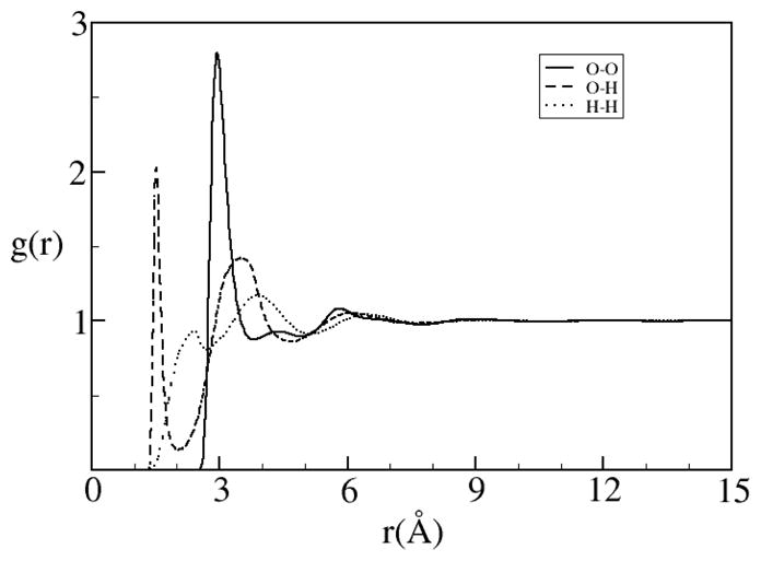
Pair correlation functions for SPC/E water calculated using DRISM theory.[78]
Figure 4.
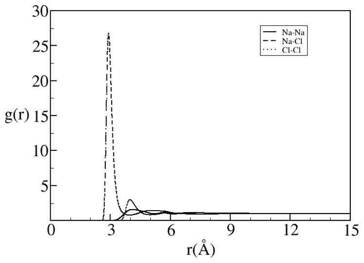
Pair correlation functions between the Na+ and Cl− ions in a 1M NaCl solution with SPC/E water.[78]
It is often the case that the solvent structure around a single complicated solute species is needed in order to understand the solvents role on the stability of the solute configurations[44]. It has been shown that solvent mediated forces play a significant role in the conformational stability of solvated molecules.
To calculate the 3D correlation functions equation II.10 can be coupled with one of the closures (HNC, PY, KH, etc.) in their 3D representation and solved iteratively with one of the numerical methods in section VII. An example is given in figure 5 for the distribution of water around water.
Figure 5 .
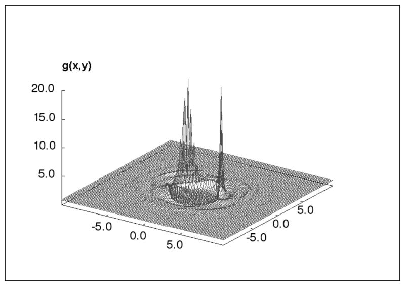
Water-oxygen site distributions in the plane through a water molecule at infinite dilution located at the origin (SPC/E water model). The large peaks are the water-oxygen sites coordinated to the hydrogen sites on the solute water molecule. Units are in Angtroms.[15]
The closure can have a significant effect on the quality of the results for certain models. Perkyns et. al. showed that the HNC closure is more accurate than the KH closure for polar fluids when compared to MD simulations for the same Hamiltonian system.[13] The KH closure significantly underestimates the magnitude of the density peaks. For models containing electrostatic sites either the approximate Ewald method[3] or the 3D exact method[13] (section IV) must be used in order to circumvent the problems associated with the long-ranged potential functions. The algorithms for solving the 3D-IEs are more computationally intensive than the 1D-IEs and require a larger amount of computer memory.
The original motivation for using the 3D-IEs was the more detailed solvent distributions they produce when applied to anisotropic solute models (compare Fig. 5 to Fig. 3). The 3D-IE studies have provided valuable information on how the solvent species distribute themselves in and around the solute molecule[13, 16, 79, 80]. Note that in figure 5 we have a cut through a three body correlation function involving the ion, a wall and the solvent.
Some of the application studies include the probabilities of the solvent and ion species around solute molecules[14, 16, 79] which include organic molecules, proteins and polypeptides[81], protein binding sites[80, 82], cavities[12, 83, 84], protein membrane channels[85], planar interfaces[18, 86–92] (see Fig. 6), and DNA[16, 93] (see Figs 7, 8 and 9). The qualitative ability of the 3D-IEs to accurately predict these distributions has been demonstrated through many comparisons with simulations and experimental studies for many solute/solvent systems [13, 17].
Figure 6 .
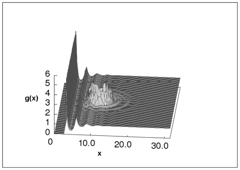
Water-Oxygen site distributions around a cation near a planar wall in a 1M NaCl solution. Units are in Angstroms from the center of surface.[18]
Figure 7 .
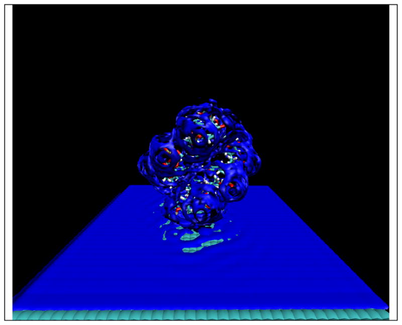
Water-oxygen site distributions around a 6-base pair AT DNA duplex near a planar surface. The iso-surface value is set to 2.8. Density fluctuations along the surface of the plane are induced by the DNA molecule.
Figure 8 .
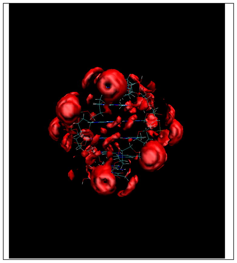
Na+ ion distribution around an 6-mer AT DNA duplex with an iso-surface value of 60.[16]
Figure 9.
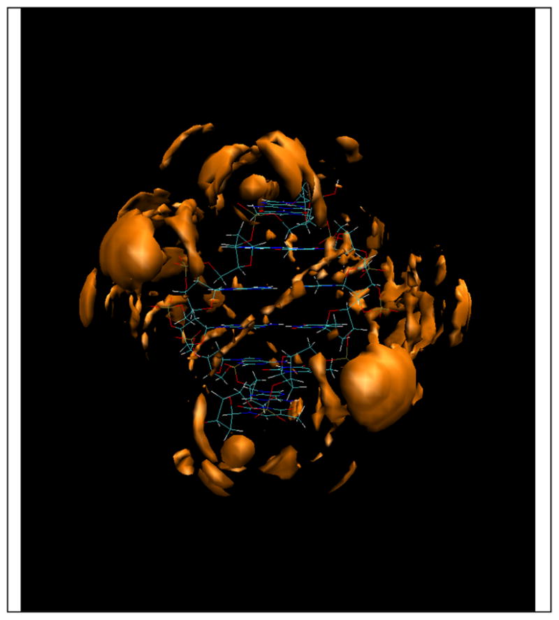
Cl− ion distribution around the 6mer-AT DNA duplex with an iso-surface value of 4.[16]
An interesting study on the ion selectivity of protein binding sites showed that the 3D-IE theory could accurately predict the discrimination of different ions (Na+, Ca+, K+) by binding sites and the results were for the most part in agreement with experiments[82]. The 3D-IEs have more recently also been able to capture the different ion selectivity in the minor and major grooves of DNA[16]. The problems of convergence of the equations for mixtures of simple ions and polyelectrolytes has largely been alleviated by the use of HNC closures (with or without approximate bridge corrections) and the use of the error function treatment shown above.
The ability to consider polyelectrolytes and their explicit distribution of both counter-ions and co-ions with respect to other chemical and geometric variables allows a range of possible applications. In figures 8 and 9 note the difference in contour levels between counter- and co-ions. Co-ion distributions have been more difficult to quantify from simulation.
The solvation of molecular complexes or clusters of species at infinite dilution has the effect of adding an external potential field to the solvent environment which significantly affects the solvent distributions within this field. These changes in the solvent distributions and the genesis of solvent interactions with the solute can have an effect on the structural stability of the solute’s configuration. Through the use of equations V.4,5, depending on the closure, the solvation free energy of the solute can be calculated and the structural stability can be analyzed.
3D-IEs have been used to assess the structural stability of several model solutes including organic compounds[19, 94, 95], hydrophobic solutes[17, 62, 96], polar molecules[96], and species as large as proteins[13, 20, 97]. These types of studies have been especially useful in the analysis of the structural stability of an ensemble of protein configurations. In one study the hydration free energy (HFE) for several protein sized models were calculated for the active form and several unfolded states[97]. It was found that the stability of the proteins could in some cases be approximately analyzed in terms of the solvent contributions to the free energy. In the same study[21] the HFE was also decomposed into its energetic and entropic components according to
| (VI.B.3) |
where the solute-solvent interaction term was calculated from the energy equation,
| (VI.B.4) |
The entropic term was calculated using a finite difference method according to the temperature derivative of the solvation free energy (eq. VI.C.3), The solvent-solvent term is difficult to calculate directly and therefore is usually calculated from the other values in equation VI.B.3 once they are known.
| (VI.B.5) |
This decomposition allowed the authors to analyze their findings in terms of the entropic and enthalpic parts of the free energy changes, which is a challenging task using molecular simulations. These parts were then further decomposed into non-electrostatic and electrostatic components to gain a complete picture of the energetic and entropic origins of each component of the solvation free energy. It was found that the HFE for these protein models is dominated by the non-electrostatic entropic part and the electrostatic enthalpic part which ultimately can provide insight into the protein folding mechanism.
One of the more interesting and useful thermodynamic properties which can be calculated using the 3D-IEs is the free energy profile with respect to any number of spatial parameters. It has been shown that the solvent contributions to the free energy profile can have a significant effect on the association of solution species [17, 98]. The free energy profile or PMF, W(r),, can be calculated by summing the direct interactions among the solute molecules, u (r), as well as the the work done on the system or the so-called cavity potential, ΔΔμ(r).
| (VI.B.6) |
The coordinate, r, can be any geometric parameter describing the change in the model. The solvent contributions to the PMF are usually taken as the difference between the configuration and a reference configuration. In the case where the parameter is the intermolecular separation the solvent contributions can be calculated according to,
where the first term is the solvation free energy of the complex structure and the last two terms are the solvation of the individual structures where the intermolecular separation would be infinity[17]. These types of studies on the free energy profiles of associating species have been done for hard spheres[99], LJ spheres[100], ions[61, 66, 101], molecules[101], ligand-protein systems[102] and hydrophobic plates[17] (Fig. 10). The PMF from the 3D-IE in these studies were for the most part in relatively good qualitative agreement with simulations for the same model system.
Figure 10.
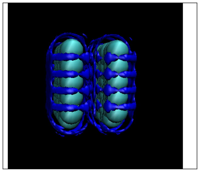
Water-oxygen site distributions around two graphene plates 7.5 Angstroms apart with an iso-surface value of 2.8 (measured center to center).[17]
In the case of the hydrophobic plates, Fig. 10, we note that the HNC closure as well as some others mentioned above were deficient in describing the drying transition, even when the drying was purely sterically induced. Thus we expect that these approximations yield hydrophobic cavities in proteins that are also wet when they should be relatively dry. This defect may be addressable with bridge functions but is as yet a problem.
VII. Numerical Methods
We would be remiss not cover some of the methods used in the solution of the liquid state integral equations described above. While this is in itself a substantial area of research it is dwarfed by the literature of differential equation solvers. We consider iterative, basis set and multi grid methods below.
A. Picard methods
Picard type iterative methods have been the most widely used routines to solve the coupled IEs presented in this article. They are fairly easy to implement compared to the other routines mentioned in this section and require the least amount of memory and computational resources. They are based on the successive iteration of the equations – an initial guess to the equations is used as the input to the solution at the next level.
| (VII.A.1) |
The Picard iterative routine does not depend on the minimization of any equation parameters to reduce the residual vector, R(r) =hi+1 (r) – hi (r). This lack of control over the iterative process can often cause the solutions to diverge for even a set of relatively non-stiff equations. One method to encourage convergence of the solutions to stiffer problems is to limit the amount of mixing of the new solution into the old solution according to successive relaxtion,
| (VII.A.2) |
where α is the mixing parameter with a typical range of (0 → 1) but this can be relaxed in proactice. When α = 0 there is no mixing of the new values into the old (stagnant) and as α → 1 the contribution of the old solution reduces to zero. Often times as equations become stiff considerable manual intervention can be required.
B. MDIIS methods
The modified direct inversion of the iterative subspace method (MDIIS) was originally developed to accelerate the convergence of numerical problems in quantum mechanics[103–105]. It has since become an invaluable tool for accelerating the convergence of the numerical solutions to the IEs in this article[51, 66, 106]. Compared to direct methods this method requires relatively small memory resources and converges more quickly than Picard methods.
To implement this method a set of basis vectors spanning an n-dimensional subspace is defined. These n-vectors are usually obtained from the iterative history and a linear combination of these vectors forms a possible solution set to the linear equations. Solutions to the linear equations are constructed using,
| (VII.B.1) |
where the coefficients, cj, are chosen to minimize a residual scalar quantity which depends on the residual vector set. The new residual vector for the solution set defined above is a linear combination of the residual vectors corresponding to the vectors in equation VII.B.1.
| (VII.B.2) |
The coefficients in the above equations are chosen to minimize the magnitude of the residual vector. To calculate these coefficients we define n independent equations from the residual vectors and one additional constraint on the coefficients. These equations are,
| (VII.B.3) |
and lead to the following set of linear equations
| (VII.B.4) |
| (VII.B.5) |
Once the coefficients are chosen they can be used to calculate the new solution vector (VII.B.1) and residual vector (VII.B.2). A mixing parameter can be used to limit the amount of the residual vector added to the solution vector for the calculation of the new solution vector.
| (VII.B.6) |
This new vector can be used to extend the dimensions of the subspace or can be used to update one of the older vectors. The basis set is updated in this manner until a solution is found where the scalar residual quantity satisfies some predetermined criterion or until the updated solutions become stagnant. If the latter is the case the entire basis set can be dumped and a new set can be formed from iteration.
C. Newton-Raphson type methods
Numerical methods based on Newton-Raphson schemes provide a direct means for minimizing a function with respect to the functions values. As long as the starting solution is within the radius of convergence the equation will converge to a minimized solution. Unlike the Picard or MDIIS methods the rate of convergence of Newton type solvers is quadratic when inside the radius of convergence. These methods are very robust; however, the solution may be a local minimum and not the global minimum that was hoped for. These numerical methods are based on solving Newton’s equation for the roots of the function F(x). Newton’s equation is,
| (VII.C.1) |
The Jacobian matrix, J, contains the derivatives of the function, F(x). The Jacobian matrix can become very large for discretized and multi-variable systems and require large amounts of memory. In addition to the storage requirements and calculating the elements, the Jacobian also must be inverted, which scales as O(n3).
Newton type numerical applications can be used in conjunction with a set of basis functions to reduce the size of the Jacobian matrix and the number of discretized equations[107, 108]. These types of methods have been applied successfully to calculate solutions to the OZ-IE for spherical species as well as solutions to the SSOZ-IE for molecular systems using 1D and 3D spatial grids[17, 107–110].
Although the implementation of Newton type methods are more involved than the Picard or MDIIS methods, the solutions to the IEs can be obtained in a fraction of the number of iterations needed by the other methods. Solutions to the equations can also be calculated in regions of the phase diagram where the other numerical methods would fail to converge. This method is especially handy when trying to calculate solutions near phase boundaries or unstable regions of the phase diagram.
An application of a Newton-type scheme to calculate the correlation functions of a system of LJ spheres in combination with the HNC closure is shown below as an example. For this system our equation set will consist of the single component OZ equation and the HNC closure. For the one-component system the OZ equation written in Fourier space is
| (VII.C.2) |
where the subscripts denote the ith point from the origin of the discretized function, t(iΔr) = ti. The other function, Fi(ci), is defined using the closure relation as,
| (VII.C.3) |
| (VII.C.4) |
where F(c) = 0 when the correct form of c and t have been obtained. Equation VII.C.4 and VII.C.2 are used to solve our Newton type equation. The next step is to calculate the Jacobian for our system of equations. The elements of the Jacobian, Jij, can be calculated by taking the full derivative of the closure and applying the chain rule.
| (VII.C.5) |
The first derivative on the right hand side of equation VII.C.4 is easily calculated and defined as,
| (VII.C.6) |
The first derivative in the second term is,
| (VII.C.7) |
To calculate the second derivative in the second term we need to define the relationship between the real space functions and the Fourier space functions. The inverse Fourier transform of the function, t, is
| (VII.C.8) |
where the values of the variables are ri = iΔr and kl = lΔk. Using equation VII.C.8 we can express the derivative as
| (VII.C.9) |
The third derivative of the second term is calculated using equation VII.C.2. The expression for this derivative is,
| (VII.C.10) |
To calculate the last derivative in the second term we can use the definition of the forward Fourier transform for c which is
| (VII.C.11) |
and the derivative of this function can be written as,
| (VII.C.12) |
After combining the derivatives, the elements of the Jacobian matrix can be defined as,
| (VII.C.13) |
Calculating the Jacobian can be an exhausting task for grids containing many points. As can be seen from equation VII.C.13 the Jacobian matrix elements depend on the current values of the correlation functions and therefore the Jacobian elements should be updated after each iteration. However, if the Jacobian elements are not changing dramatically the Jacobian can be used for several iterations before being updated. This can greatly increase the speed of the computation.
The other limiting step in the efficiency of these types of applications is the inversion of the Jacobian matrix. Methods based on the Gauss-Jordan elimination or LU decomposition require a large number of iterations being proportional to n3. This makes the application of these methods almost impossible for large grids, such as 3D grids. To increase the efficiency of this step routines based on Krylov space methods have been utilized[17, 111, 112]. Krylov space methods iteratively build an approximate solution to the linear equation, which scales proportional to n2 for each iteration. If the number of iterations is low one can see how this method could increase the speed of convergence of the equations.
These methods can be used in combination in a variety of ways. Newton-Raphson methods can be used on a coarse grid and the details can be filled in with other less costly methods. Numerical stability in an iterative solution requires attention to transfers of the functions between the coarse and fine grids. Many multilevel alternatives exist and can greatly improve efficiency.[111, 113]
VIII. Conclusions
Integral equations have matured from the first applications of 1D-IEs to simple homogenous hard sphere systems to current day applications which involve 3D-IEs for large inhomogeneous systems in ionic aqueous solvents. However still many approximations have been made which often compromised the integrity of the IEs. These approximations limit the potential of the IEs in terms of thermodynamic predictions, but at the same time have allowed for their expansion to include a wide scope of systems. Even with the current level of theory the IEs have become an important tool for the study of dense fluids and their full potential has not been reached yet.
Some of the progress currently being made includes methods to solve the angular dependent correlation functions for complex systems such as water[114]. There are also efforts being conducted to calculate the correlation functions using variational methods to minimizing the free energy of the system[115]. A promising example is given by recent advances to quantitatively improve upon the thermodynamics and predicted dielectric constant of molecular fluids using molecular angular expansions in diagrammatically proper, site-site, integral equation theory[26]. The possibility of an equation predictive of the dielectric properties for any molecular mechanics potential is tantalizing.
Acknowledgments
The authors would like to thank the Robert A. Welch (E-1028) foundation and the National Institutes of Health (GM-37657 and GM-066813) for partial support of this work. J.J.H would also like to thank the Keck Center for Interdisciplinary Bioscience of the Gulf Coast Consortia for a fellowship.
References
- 1.Hansen JP, McDonald IR. Theory of Simple Liquids. San Diego: Academic Press; 1986. [Google Scholar]
- 2.Monson PA, Morriss GP. Recent progress in the statistical mechanics of interaction site fluids. Advances in Chemical Physics. 1990;77:451–550. [Google Scholar]
- 3.Hirata F. Molecular Theory of Solvation. In: Mezey PG, editor. Understanding Chemical Reactivity. Vol. 24. Kluwer Academic Publishers; Dordrecht: 2003. [Google Scholar]
- 4.Hoeye JS, Lebowitz JL, Stell G. Generalized mean spherical approximations for polar and ionic fluids. J Chem Phys. 1974;61(8):3253–60. [Google Scholar]
- 5.Waisman EM, Lebowitz JL. Mean spherical model integral equation for charged hard spheres. I. Method of solution. Journal of Chemical Physics. 1972;56(6):3086–93. [Google Scholar]
- 6.Waisman E, Lebowitz JL. Exact solution of an integral equation for the structure of a primitive model of electrolytes. J Chem Phys. 1970;52(8):4307–9. [Google Scholar]
- 7.Chandler D, Andersen HC. Optimized cluster expansions for classical fluids. II. Theory of molecular liquids. Journal of Chemical Physics. 1972;57(5):1930–7. [Google Scholar]
- 8.Andersen HC, Chandler D, Weeks JD. Optimized cluster expansions for classical fluids. III. Applications to ionic solutions and simple liquids. Journal of Chemical Physics. 1972;57(7):2626–31. [Google Scholar]
- 9.Hirata F, Rossky PJ. An extended RISM equation for molecular polar fluids. Chemical Physics Letters. 1981;83(2):329–34. [Google Scholar]
- 10.Hirata F, Pettitt BM, Rossky PJ. Application of an extended RISM equation to dipolar and quadrupolar fluids. Journal of Chemical Physics. 1982;77(1):509–20. [Google Scholar]
- 11.Hirata F, Rossky PJ, Pettitt BM. The interionic potential of mean force in a molecular polar solvent from an extended RISM equation. Journal of Chemical Physics. 1983;78(6 Pt 2):4133–44. [Google Scholar]
- 12.Beglov D, Roux B. Numerical solution of the hypernetted chain equation for a solute of arbitrary geometry in three dimensions. Journal of Chemical Physics. 1995;103(1):360–4. [Google Scholar]
- 13.Perkyns JS, et al. Protein solvation from theory and simulation: Exact treatment of Coulomb interactions in three-dimensional theories. J Chem Phys. 2009;132(6):064106/1–064106/13. doi: 10.1063/1.3299277. [DOI] [PMC free article] [PubMed] [Google Scholar]
- 14.Ikeguchi M, Doi J. Direct numerical solution of the Ornstein-Zernike integral equation and spatial distribution of water around hydrophobic molecules. J Chem Phys. 1995;103(12):5011–5017. [Google Scholar]
- 15.Beglov D, Roux B. Integral Equation To Describe the Solvation of Polar Molecules in Liquid Water. Journal of Physical Chemistry B. 1997;101(39):7821–7826. [Google Scholar]
- 16.Howard JJ, Lynch GC, Pettitt BM. Ion and Solvent Density Distributions around Canonical B-DNA from Integral Equations. The Journal of Physical Chemistry B. 2011;115(3):547–556. doi: 10.1021/jp107383s. [DOI] [PMC free article] [PubMed] [Google Scholar]
- 17.Howard JJ, et al. Integral Equation Study of the Hydrophobic Interaction between Graphene Plates. Journal of Chemical Theory and Computation. 2008;4(11):1928–1939. doi: 10.1021/ct8002817. [DOI] [PMC free article] [PubMed] [Google Scholar]
- 18.Howard JJ, Perkyns JS, Pettitt BM. The Behavior of Ions near a Charged Wall— Dependence on Ion Size, Concentration, and Surface Charge. The Journal of Physical Chemistry B. 2010;114(18):6074–6083. doi: 10.1021/jp9108865. [DOI] [PMC free article] [PubMed] [Google Scholar]
- 19.Kovalenko A, Hirata F, Kinoshita M. Hydration structure and stability of Met-enkephalin studied by a three-dimensional reference interaction site model with a repulsive bridge correction and a thermodynamic perturbation method. Journal of Chemical Physics. 2000;113(21):9830–9836. [Google Scholar]
- 20.Imai T, et al. A theoretical analysis on hydration thermodynamics of proteins. Journal of Chemical Physics. 2006;125(2):024911/1–024911/7. doi: 10.1063/1.2213980. [DOI] [PubMed] [Google Scholar]
- 21.Imai T, et al. Three-Dimensional Distribution Function Theory for the Prediction of Protein-Ligand Binding Sites and Affinities: Application to the Binding of Noble Gases to Hen Egg-White Lysozyme in Aqueous Solution. Journal of Physical Chemistry B. 2007;111(39):11585–11591. doi: 10.1021/jp074865b. [DOI] [PubMed] [Google Scholar]
- 22.Dyer KM, Perkyns JS, Pettitt BM. Effective density terms in proper integral equations. Journal of Chemical Physics. 2005;123(20):204512/1–204512/11. doi: 10.1063/1.2116987. [DOI] [PMC free article] [PubMed] [Google Scholar]
- 23.Dyer KM, Perkyns JS, Pettitt BM. A site-renormalized molecular fluid theory. Journal of Chemical Physics. 2007;127(19):194506/1–194506/14. doi: 10.1063/1.2785188. [DOI] [PMC free article] [PubMed] [Google Scholar]
- 24.Perkyns J, Dyer K, Pettitt BM. Computationally useful bridge diagram series. II. Diagrams in h-bonds. Journal of Chemical Physics. 2002;116(21):9404–9412. [Google Scholar]
- 25.Dyer K, Perkyns J, Pettitt BM. Computationally useful bridge diagram series. III. Lennard-Jones mixtures. Journal of Chemical Physics. 2002;116(21):9413–9421. [Google Scholar]
- 26.Dyer KM, et al. A molecular site-site integral equation that yields the dielectric constant. J Chem Phys. 2008;129(10):104512/1–104512/9. doi: 10.1063/1.2976580. [DOI] [PMC free article] [PubMed] [Google Scholar]
- 27.McQuarrie DA. Statistical Mechanics. Vol. 13 Sausalito: University Science Books; 2000. [Google Scholar]
- 28.Baer S, Lebowitz JL. Convergence of fugacity expansion and bounds on molecular distributions for mixtures. J Chem Phys. 1964;40(12):3474–8. [Google Scholar]
- 29.Helfand E, et al. Scaled particle theory of fluids. J Chem Phys. 1960;33:1379–85. [Google Scholar]
- 30.Reiss H, Frisch HL, Lebowitz JL. Statistical mechanics of rigid spheres. Journal of Chemical Physics. 1959;31:369–80. [Google Scholar]
- 31.Huisman WJ, et al. A new x-ray diffraction method for structural investigations of solid-liquid interfaces. Rev Sci Instrum FIELD Full Journal Title:Review of Scientific Instruments. 1997;68(11):4169–4176. [Google Scholar]
- 32.Bausenwein T, et al. Structure and intermolecular interactions in fluid ammonia: an investigation by neutron diffraction at high pressure, statistical-mechanical calculations and computer simulations. Journal of Chemical Physics. 1994;101(1):672–82. [Google Scholar]
- 33.Ackermann PG, Mayer JE. Determination of Molecular Structure by Electron Diffraction. Journal of Chemical Physics. 1936;4:377–381. [Google Scholar]
- 34.Ornstein LS, Zernike F. Proc R Acad Sci. Vol. 17. Amsterdam: 1914. p. 793. [Google Scholar]
- 35.Hiroike K. Radial Distribution Function of Fluids II. Journal of the Physical Society. 1957;12(8):864–873. [Google Scholar]
- 36.Frigo M, Johnson SG. The Design and Implementation of FFTW3. Proceedings fo the IEEE. 2005;93(2):216–231. [Google Scholar]
- 37.Hansen JP, McDonald IR. Theory of Simple Liquids. London: Academic; 1976. [Google Scholar]
- 38.Blum L, Torruella AJ. Invariant Expansion for Two-Body Correlations: Thermodynamic Functions, Scattering, and the Ornstein-Zernike Equation. Journal of Chemical Physics. 1972;56(1):303–310. [Google Scholar]
- 39.Fries PH, Patey GN. The solution of the hypernetted-chain approximation for fluids of nonspherical particles. A general method with application to dipolar hard spheres. Journal of Chemical Physics. 1985;82(1):429–40. [Google Scholar]
- 40.Perkyns JS, Fries PH, Patey GN. The solution of the reference hypernetted-chain approximation for fluids of hard spheres with dipoles and quadrupoles. Molecular Physics. 1986;57(3):529–42. [Google Scholar]
- 41.Chandler D. Derivation of an integral equation for pair correlation functions in molecular fluids. Journal of Chemical Physics. 1973;59(5):2742–6. [Google Scholar]
- 42.Chandler D, Joslin CG, Deutch JM. Calculation of the dielectric constant of polyatomic fluids with the interaction site formalism. Molecular Physics. 1982;47(4):871–9. [Google Scholar]
- 43.Ng KC. Hypernetted chain solutions for the classical one component plasma up to G = 7000. Journal of Chemical Physics. 1974;61(7):2680–9. [Google Scholar]
- 44.Pettitt BM, Rossky PJ. Alkali halides in water: ion-solvent correlations and ion-ion potentials of mean force at infinite dilution. Journal of Chemical Physics. 1986;84(10):5836–44. [Google Scholar]
- 45.Nishiyama K, Hirata F, Okada T. Solute-Shape Dependence in Solvation Dynamics: Investigated by RISM Theory. Journal of Molecular Liquids. 2002;96–97:391–395. [Google Scholar]
- 46.Kinoshita M, Okamoto Y, Hirata F. Solvent effects on conformational stability of peptides: RISM analyses. Journal of Molecular Liquids. 2001;90(1–3):195–204. [Google Scholar]
- 47.Sato H, Hirata F. Equilibrium and Nonequilibrium Solvation Structure of Hexaammineruthenium (II, III) in Aqueous Solution: Ab Initio RISM-SCF Study. Journal of Physical Chemistry A. 2002;106(10):2300–2304. [Google Scholar]
- 48.Yoshido K, et al. Structure of tert-Butyl Alcohol-Water Mixtures Studied by the RISM Theory. J Phys Chem B. 2002;106:5042–5049. [Google Scholar]
- 49.Lee JY, Yoshida N, Hirata F. Conformational Equilibrium of 1,2-Dichloroethane in Water: Comparison of PCM and RISM-SCF Methods. Journal of Physical Chemistry B. 2006;110(32):16018–16025. doi: 10.1021/jp0606762. [DOI] [PubMed] [Google Scholar]
- 50.Marlow GE, Perkyns JS, Pettitt BM. Salt effects in peptide solutions: theory and simulations. Chemical Reviews (Washington, DC, United States) 1993;93(7):2503–21. [Google Scholar]
- 51.Kovalenko A, Ten-No S, Hirata F. Solution of three-dimensional reference interaction site model and hypernetted chain equations for simple point charge water by modified method of direct inversion in iterative subspace. Journal of Computational Chemistry. 1999;20(9):928–936. [Google Scholar]
- 52.Ladanyi BM, Chandler D. New type of cluster theory for molecular fluids. Interaction site cluster expansion. Journal of Chemical Physics. 1975;62(11):4308–24. [Google Scholar]
- 53.Chandler D, Silbey R, Ladanyi BM. New and proper integral equations for site-site equilibrium correlations in molecular fluids. Molecular Physics. 1982;46(6):1335–45. [Google Scholar]
- 54.Rossky PJ, Chiles RA. A complete integral equation formulation in the interaction site formalism. Molecular Physics. 1984;51(3):661–74. [Google Scholar]
- 55.Stell G. The Percus-Yevick equation for the radial distribution function of a fluid. Physica (The Hague) 1963;29(5):517–34. [Google Scholar]
- 56.Percus JK, Yevick GJ. Analysis of classical statistical mechanics by means of collective coordinates. Physical Review. 1958;110:1–13. [Google Scholar]
- 57.Broyles AA, Chung SU, Sahlin HL. Comparison of radial distribution functions from integral equations and Monte Carlo. Journal of Chemical Physics. 1962;37:2462–9. [Google Scholar]
- 58.Watts RO. Hypernetted-chain approximation applied to a modified Lennard-Jones fluid. Journal of Chemical Physics. 1969;50(3):1358–65. [Google Scholar]
- 59.van Leeuwen JMJ, Groeneveld J, de Boer J. New method for the calculation of the pair correlation function. I Physica. 1959;25(7–12):792–808. [Google Scholar]
- 60.Lebowitz JL, Percus JK. Mean spherical model for lattice gases with extended hard cores and continuum fluids. Phys Rev FIELD Full Journal Title:Physical Review. 1966;144(1):251–8. [Google Scholar]
- 61.Kovalenko A, Hirata F. Potentials of mean force of simple ions in ambient aqueous solution. II. Solvation structure from the three-dimensional reference interaction site model approach, and comparison with simulations. Journal of Chemical Physics. 2000;112(23):10403–10417. [Google Scholar]
- 62.Kovalenko A, Hirata F. Hydration free energy of hydrophobic solutes studied by a reference interaction site model with a repulsive bridge correction and a thermodynamic perturbation method. J Chem Phys. 2000;113(7):2793–2805. [Google Scholar]
- 63.Perkyns J, Pettitt BM. A dielectrically consistent interaction site theory for solvent-electrolyte mixtures. Chemical Physics Letters. 1992;190(6):626–630. [Google Scholar]
- 64.Pettitt BM, Rossky PJ. Integral equation predictions of liquid state structure for waterlike intermolecular potentials. Journal of Chemical Physics. 1982;77(3):1451–7. [Google Scholar]
- 65.Allnatt AR. Mol Phys. 1964;8:533. [Google Scholar]
- 66.Kovalenko A, Hirata F. Potentials of mean force of simple ions in ambient aqueous solution. I. Three-dimensional reference interaction site model approach. Journal of Chemical Physics. 2000;112(23):10391–10402. [Google Scholar]
- 67.Hunenberger PH, McCammon JA. Ewald artifacts in computer simulations of ionic solvation and ion-ion interaction: A continuum electrostatics study. J Chem Phys FIELD Full Journal Title:Journal of Chemical Physics. 1999;110(4):1856–1872. [Google Scholar]
- 68.Mayer JE, Harrison SF. Statistical Mechanics of Condensing Systems. III. Journal of Chemical Physics. 1938;6:87–100. [Google Scholar]
- 69.Andersen HC, Chandler D. Optimized cluster expansions for classical fluids. I. General theory and variational formulation of the mean spherical model and hard sphere Percus-Yevick equations. Journal of Chemical Physics. 1972;57(5):1918–29. [Google Scholar]
- 70.Mayer JE. The Statisical Mechanics of Condensing Systems. I. Journal of Chemical Physics. 1937;5:67–73. [Google Scholar]
- 71.Mayer JE, Ackermann PG. The Statistical Mechanics of Condensing Systems. II. Journal of Chemical Physics. 1937;5:74–83. [Google Scholar]
- 72.Streeter SF, Mayer JE. The Statistical Mechanics of Condensing Systems IV. The Treatment of a System of Constant Energy. Journal of Chemical Physics. 1939;7:1025–1038. [Google Scholar]
- 73.Morita T, Hiroike K. A New Approach to the Theory of Classical Fluids. III. Progress of Theoretical Physics. 1961;25(4):537–578. [Google Scholar]
- 74.Daniel Trzesniak A-PEKWFvG. A Comparison of Methods to Compute the Potential of Mean Force. Chem Phys Chem. 2007;8(1):162–169. doi: 10.1002/cphc.200600527. [DOI] [PubMed] [Google Scholar]
- 75.Rossky PJ, Pettitt BM, Stell G. The coupling of long and short range correlations in ISM liquids. Molecular Physics. 1983;50(6):1263–71. [Google Scholar]
- 76.Stell G, Patey GN, Hoeye JS. Dielectric constants of fluid models: statistical mechanical theory and its quantitative implementation. Advances in Chemical Physics. 1981;48:183–328. [Google Scholar]
- 77.Chandler D. The dielectric constant and related equilibrium properties of molecular fluids: interaction site cluster theory analysis. Journal of Chemical Physics. 1977;67(3):1113–24. [Google Scholar]
- 78.Perkyns J, Pettitt BM. A site-site theory for finite concentration saline solutions. Journal of Chemical Physics. 1992;97(10):7656–7666. [Google Scholar]
- 79.Kovalenko A, Hirata F. Three-dimensional density profiles of water in contact with a solute of arbitrary shape: a RISM approach. Chemical Physics Letters. 1998;290(1,2,3):237–244. [Google Scholar]
- 80.Imai T, et al. Water Molecules in a Protein Cavity Detected by a Statistical-Mechanical Theory. J Am Chem Soc. 2005;127(44):15334–15335. doi: 10.1021/ja054434b. [DOI] [PubMed] [Google Scholar]
- 81.Harano Y, et al. Theoretical study for partial molar volume of amino acids and polypeptides by the three-dimensional reference interaction site model. Journal of Chemical Physics. 2001;114(21):9506–9511. [Google Scholar]
- 82.Yoshida N, et al. Selective Ion-Binding by Protein Probed with the 3D-RISM Theory. J Am Chem Soc. 2006;128(37):12042–12043. doi: 10.1021/ja0633262. [DOI] [PubMed] [Google Scholar]
- 83.Imai T, et al. Locating Missing Water Molecules in Protein Cavities by the Three-Dimensional Reference Interaction Site Model Theory of Molecular Solvation. Vol. 66. Wiley InterScience; 2006. pp. 804–813. [DOI] [PubMed] [Google Scholar]
- 84.Imai T, et al. Locating missing water molecules in protein cavities by the three-dimensional reference interaction site model theory of molecular solvation. Proteins: Structure, Function, and Bioinformatics. 2007;66(4):804–813. doi: 10.1002/prot.21311. [DOI] [PubMed] [Google Scholar]
- 85.Phongphanphanee S, Yoshida N, Hirata F. On the Proton Exclusion of Aquaporins: A Statistical Mechanics Study. J Am Chem Soc. 2008;130(5):1540–1541. doi: 10.1021/ja077087+. [DOI] [PubMed] [Google Scholar]
- 86.Chen ZM, Pettitt BM. Non-isotropic solution of an OZ equation: matrix methods for integral equations. Computer Physics Communications. 1995;85(2):239–50. [Google Scholar]
- 87.Kinoshita M, Hirata F. Application of the reference interaction site model theory to analysis on surface-induced structure of water. Journal of Chemical Physics. 1996;104(21):8807–8815. [Google Scholar]
- 88.Akiyama R, Hirata F. Theoretical study for water structure at highly ordered surface: Effect of surface structure. Journal of Chemical Physics. 1998;108(12):4904–4911. [Google Scholar]
- 89.Kovalenko A, Hirata F. Self-consistent description of a metal-water interface by the Kohn-Sham density functional theory and the three-dimensional reference interaction site model. Journal of Chemical Physics. 1999;110(20):10095–10112. [Google Scholar]
- 90.Shapovalov V, et al. Liquid structure at metal oxide-water interface. accuracy of a three-dimensional RISM methodology. Chemical Physics Letters. 2000;320(1,2):186–193. [Google Scholar]
- 91.Kovalenko A, Hirata F. Self-consistent, Kohn-Sham DFT and three-dimensional RISM description of a metal-molecular liquid interface. Journal of Molecular Liquids. 2001;90(1–3):215–224. [Google Scholar]
- 92.Kovalenko A, Hirata F. A molecular theory of liquid interfaces. Physical Chemistry Chemical Physics. 2005;7(8):1785–1793. doi: 10.1039/b416615a. [DOI] [PubMed] [Google Scholar]
- 93.Yonetani Y, et al. Comparison of DNA hydration patterns obtained using two distinct computational methods, molecular dynamics simulation and three-dimensional reference interaction site model theory. Journal of Chemical Physics. 2008;128(18):185102/1–185102/9. doi: 10.1063/1.2904865. [DOI] [PubMed] [Google Scholar]
- 94.Miyata T. Reference interaction site model study on the anomeric equilibrium of D-glucose in aqueous solution. Condensed Matter Physics. 2007;10:433–438. [Google Scholar]
- 95.Miyata T, Hirata F. Combination of molecular dynamics method and 3D-RISM theory for conformational sampling of large flexible molecules in solution. Journal of Computational Chemistry. 2008;29(6):871–882. doi: 10.1002/jcc.20844. [DOI] [PubMed] [Google Scholar]
- 96.Du Q, Beglov D, Roux B. Solvation Free Energy of Polar and Nonpolar Molecules in Water: An Extended Interaction Site Integral Equation Theory in Three Dimensions. Journal of Physical Chemistry B. 2000;104(4):796–805. [Google Scholar]
- 97.Imai T, et al. Theoretical analysis on changes in thermodynamic quantities upon protein folding: Essential role of hydration. Journal of Chemical Physics. 2007;126(22):225102/1–225102/9. doi: 10.1063/1.2743962. [DOI] [PubMed] [Google Scholar]
- 98.Choudhury N, Pettitt BM. Enthalpy-Entropy Contributions to the Potential of Mean Force of Nanoscopic Hydrophobic Solutes. Journal of Physical Chemistry B. 2006;110(16):8459–8463. doi: 10.1021/jp056909r. [DOI] [PMC free article] [PubMed] [Google Scholar]
- 99.Kinoshita M, Harano Y, Akiyama R. Changes in thermodynamic quantities upon contact of two solutes in solvent under isochoric and isobaric conditions. Journal of Chemical Physics. 2006;125(24):244504/1–244504/7. doi: 10.1063/1.2403873. [DOI] [PubMed] [Google Scholar]
- 100.Tomonari S, Hideo S. Integral equation study of hydrophobic interaction: A comparison between the simple point charge model for water and a Lennard-Jones model for solvent. The Journal of Chemical Physics. 2007;126(14):144508. doi: 10.1063/1.2718520. [DOI] [PubMed] [Google Scholar]
- 101.Maruyama Y, Matsugami M, Ikuta Y. Probing cations recognized by a crown ether with the 3D-RISM theory. II. 18-crown-6 ether. Condensed Matter Physics. 2007;51:315–322. [Google Scholar]
- 102.Yoshida N, et al. Molecular Recognition in Biomolecules Studied by Statistical-Mechanical Integral-Equation Theory of Liquids. Journal of Physical Chemistry B. 2009;113(4):873–886. doi: 10.1021/jp807068k. [DOI] [PubMed] [Google Scholar]
- 103.Pulay P. Convergence acceleration of iterative sequences. The case of SCF iteration. Chemical Physics Letters. 1980;73(2):393–8. [Google Scholar]
- 104.Pulay P. Improved SCF convergence acceleration. Journal of Computational Chemistry. 1982;3(4):556–60. [Google Scholar]
- 105.Hamilton TP, Pulay P. Direct inversion in the iterative subspace (DIIS) optimization of open-shell, excited-state, and small multiconfiguration SCF wave functions. Journal of Chemical Physics. 1986;84(10):5728–34. [Google Scholar]
- 106.Kovalenko A, Hirata F. Potential of Mean Force between Two Molecular Ions in a Polar Molecular Solvent: A Study by the Three-Dimensional Reference Interaction Site Model. The Journal of Physical Chemistry B. 1999;103(37):7942–7957. [Google Scholar]
- 107.Abernethy GM, Gillian MJ. A new method of solving the HNC equation for ionic liquids. Molecular Physics. 1980;39(4):839–847. [Google Scholar]
- 108.Gillan MJ. A new method of solving the liquid structure integral equations. Molecular Physics. 1979;38(6):1781–1794. [Google Scholar]
- 109.Booth MJ, et al. Efficient solution of liquid state integral equations using the Newton-GMRES algorithm. Computer Physics Communications. 1999;119(2–3):122–134. [Google Scholar]
- 110.Peplow AT, Beardmore RE, Bresme F. Algorithms for the computation of solutions of the Ornstein-Zernike equation. Physical Review E: Statistical, Nonlinear, and Soft Matter Physics. 2006;74(4–2):046705/1–046705/11. doi: 10.1103/PhysRevE.74.046705. [DOI] [PubMed] [Google Scholar]
- 111.Kelley CT. Solving Nonlinear Equations with Newton’s Method. Philadelphia: Society for Industrial and Applied Mathematics; 2003. p. 118. [Google Scholar]
- 112.Saad Y, Schultz MH. GMRES: A Generalized Minimal Residual Algorithm for Solving Nonsymmetric Linear Systems. SIAM J SCI STAT COMPUT. 1986;7(3):856–869. [Google Scholar]
- 113.Kelley CT, Pettitt BM. A fast solver for the Ornstein-Zernike Equations. J Comp Phys. 2004;197/2:491–501. [Google Scholar]
- 114.Dyer KM, Pettitt BM, Stell G. Systematic investigation of theories of transport in the Lennard-Jones fluid. Journal of Chemical Physics. 2007;126(3):034502/1–034502/9. doi: 10.1063/1.2424714. [DOI] [PMC free article] [PubMed] [Google Scholar]
- 115.Marucho M, Montgomery Pettitt B. Optimized theory for simple and molecular fluids. Journal of Chemical Physics. 2007;126(12):124107/1–124107/9. doi: 10.1063/1.2711205. [DOI] [PMC free article] [PubMed] [Google Scholar]