Bayesian tracking of intracranial pressure signal morphology

Abstract

Background

The waveform morphology of intracranial pressure (ICP) pulses holds essential informations about intracranial and cerebrovascular pathophysiological variations. Most of current ICP pulse analysis frameworks process each pulse independently and therefore do not exploit the temporal dependency existing between successive pulses. We propose a probabilistic framework that exploits this temporal dependency to track ICP waveform morphology in terms of its three peaks.

Material

ICP and electrocardiogram (ECG) signals were recorded from a total of 128 patients treated for various intracranial pressure related conditions.

Methods

The tracking is posed as inference in a graphical model that associates a random variable to the position of each peak. A key contribution is to exploit a nonparametric Bayesian inference algorithm that offers robustness and real time performance. A simple, yet effective learning procedure estimates the statistical, nonlinear, dependencies between the peaks in a nonparametric way using evidence collected from manually annotated pulses.

Results

Experiments demonstrate the effectiveness of the tracking framework on real ICP pulses and its robustness to occlusion and missing peaks. On artificialy distorted ICP sequences, the average error in latency in comparision with MOCAIP detector was reduced as follows: 11.88–8.09 ms, 11.80–6.90 ms, and 11.76–7.46 ms for the first, second, and third peak, respectively.

Conclusion

The proposed tracking algorithm sucessfuly increases the temporal resolution of detecting ICP pulse morphological changes from the minute-level to the beat-level.

1. Introduction

The treatment of traumatic brain injuries (TBI) in critical care unit, as well as other neurological disorders, relies on the continuous monitoring of intracranial pressure (ICP) (i.e. the sum of the pressures exerted within the craniospinal axis system) [1]. It is known that the management of ICP can attenuate secondary brain injuries and improve chances of recovery.

While current clinical protocols generally rely on the continuous measurement of the mean ICP, recent works have demonstrated that the morphology of ICP waveform also holds essential informations about the intracranial adaptive capacity, and even the outcome of head injured patients [2,3]. For example, it has been shown that variations of the ICP pulse morphology are linked to the development of intracranial hypertension [4,5] and cerebral vasospasm [6], acute changes in the cerebral blood carbon dioxide (CO₂) levels [7,8], changes in the craniospinal compliance [9], decreased cerebral blood flow [10], and elevated ICP [11]. Therefore, the extraction of morphological features may provide insight to monitor and to understand ICP in an automatic fashion with the ultimate goal of improving the treatment of pathophysiological intracranial and cerebrovascular dynamics.

Special attention has recently been drawn from several research groups, including ours, to develop peak recognition algorithms for ICP pulses [12-15]. ICP pulses, which are typically triphasic [7] (see Fig. 1), can exhibit irregular variations in their shape that make the recognition of their three peaks very challenging. In addition, the ICP signal is usually affected by noise and various artifacts. To obtain robustness to these perturbations, MOCAIP [13] (Morphological Clustering and Analysis of ICP Pulse) extracts a dominant pulse obtained by clustering 2 min segments of ICP. In [12], different filters are applied to remove high and low frequency noise. However, these pre-processing steps come at computational cost, and unlike the tracking of mean ICP, real-time ICP pulse analysis is no longer possible.

Fig. 1.

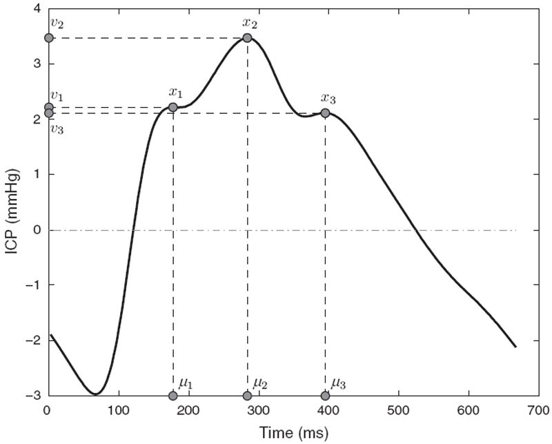
Illustration of three peaks x₁, x₂, x₃ detected on an ICP pulse together with their corresponding latency μ₁, μ₂, μ₃ and ICP elevation v₁, v₂, v₃.

This paper tackles this problem by proposing a probabilistic framework to track ICP peaks in real time that exploits temporal dependencies between successive peaks. The tracking is posed as inference in a graphical model that associates a continuous random variable to the position of each of the three peaks, in terms of their latency within the pulse and pressure elevation. A key contribution is to exploit an efficient nonparametric Bayesian inference algorithm, nonparametric belief propagation (NBP) [16]. NBP was successfully used in computer vision to track hands, people, cars, and to recognize objects. A simple, yet effective learning procedure estimates the statistical, nonlinear, dependencies between the peaks in a nonparametric way using kernel density estimation (KDE) from resampled evidence collected from manually annotated pulses.

The model is evaluated on real ICP data sampled from a large database of ICP signals collected from 128 neurosurgical patients. In addition, to quantify the peak tracking accuracy, we simulate artificial trends of peak position changes from randomly extracted pulses. The accuracy on two types of trends (sinusoidal trend, and phase multiplication), allow us to investigate how well peak tracking techniques work on ICP sequences with known trend.

2. Methods

2.1. Data source and pre-processing

The dataset of ICP signals originates from the UCLA Neurosurgery Medical Center and its usage in the present study was approved by the UCLA Internal Review Board. It is a large, representative dataset that is reasonably distributed across gender, age, and type of patients (admitted to the intensive care unit (ICU) or not (NON-ICU)).

The ICP and electrocardiogram (ECG) signals were acquired from 128 patients treated for various intracranial pressure related conditions. ICP and intraparenchymal pressure (IPP) were monitored continuously either using Codman microsensors (Codman and Schurtleff, Raynaud, MA) placed in the right frontal lobe (IPP), or using a sensor placed in the ventricle. Although, IPP as measured in the right frontal lobe may not be strictly equivalent to the ICP measured in the cerebrospinal fluid, several works [17-19] have shown that the pressure waveform can reasonably be considered as equivalent, no matter where it is measured in the brain. In this work, ICP refers indifferently to ICP (measured inside the ventricle) and IPP. Signals were recorded from bedside monitors using corporate data acquisition systems at a sampling frequency of 400 Hz. A total of 275 signal segments were extracted, whose length range from 30 min to 5 h. The continuous ICP signal was split into a series of individual ICP pulses (i.e. cardiac cycle) using a pulse extraction technique [20] that exploits an ECG QRS detection [21] as reference.

Because peak recognition methods [13,22,23] cannot usually process these raw ICP pulses reliably due to the noise and artifacts originating from the acquisition process, a more robust dominant pulse was extracted from a 3-min sequence of consecutive ICP pulses using hierarchical clustering [24]. The chosen dominant pulse corresponds to the centroid of the largest cluster. The ICP recordings were pre-processed to produce a representative set of 75,717 dominant pulses, of which 67,719 had three peaks. Note that the proposed tracking method will perform directly on raw ICP pulses, but dominant pulses are required to evaluate and to train peak detectors (such as MOCAIP).

Peak candidates are used by peak detectors and are located at curve inflections of the ICP pulse. Using the second derivative of the signal, the pulse is segmented into concave and convex regions. A peak is said to occur at the intersection of a convex to a concave region on a rising edge of ICP pulse, or at the intersection of a concave to a convex region on the descending edge of the pulse. To establish the groundtruth, experienced researchers annotates each dominant pulse by selecting manually the position of the three peaks (p₁, p₂, and p₃) among the peak candidates.

2.2. Problem formulation

We assume that the tracking framework is presented with a series of raw pulses S_t=1…n that are continuously extracted from the ICP signal. Each ICP peak i is characterized by a state x_t,i in the model. Because an ICP pulse is triphasic, the model consists of three distinct states [x_t,1, x_t,2, x_t,3] that correspond to the position of the three peaks at time t. A state x_t,i = {μ_t,i, v_t,i} is two-dimensional that defines the latency μ_t,i ∈ ℝ, and the ICP elevation v_t,i ∈ ℝ of the peak.

To each state x_t,i is associated an observation y_t,i, directly obtained from the current pulse, that depicts the position of the peak within the current pulse. It differs from the state x_t,i in the sense that it comes from peak detectors that can be affected by noise and transient artifacts present in the current pulse, whereas the value x_t,i is obtained through inference, thus believed to be more robust.

The tracking model is assumed to follow the general properties of a Markov Chain. This means that the probability of a state x_t,i at time t given all the states available so far x_1…t−1,i depends only the previous state x_t−1,i,

$$p(x_{t,i}\mid x_{\{1\dots t-1\},i})=p(x_{t,i}\mid x_{t-1,i})$$ (1)

where p(x_t,1∣x_t−1,1) represents the temporal dependency between successive states of the first peak.

By introducing observations y_t,i in the model, it becomes a hidden markov model (HMM), and the posterior marginal of the first peak can be written in the following recursive fashion,

$$p(x_{t,1}\mid y_{\{1\dots t\},1})\propto p(y_{t,1}\mid x_{t,1})\mathit{\int }p(x_{t,1}\mid x_{t-1,1})\times p(x_{t-1,1}\mid y_{\{1\dots t-1\},1}){\mathit{dx}}_{t-1,1}$$ (2)

where p(y_t,i∣x_t,i) is the likelihood.

The formulation of Eq. (2) assumes that the distribution of the three peaks are independent. However, Fig. 2, which plots the co-occurence of latency of the three peaks collected from training pulses, shows that this hypothesis is not valid. There exists a non-linear dependency between the different peaks that should also be included in the Bayesian model. Therefore, the posterior marginal can then be written as,

$$\begin{array}{l}p(x_{t,1}\mid y_{\{1\dots t\}})\propto p(y_{t,1}\mid x_{t,1})\mathit{\int }p(x_{t,1}\mid x_{t-1,1})\\ \times p(x_{t-1,1}\mid y_{\{1\dots t-1\}})d{x}_{t-1,1}\mathit{\int }p(x_{t,1}\mid x_{t,2})\\ \times p(x_{t,2}\mid y_{\{1\dots t\}})d{x}_{t,2}\mathit{\int }p(x_{t,1}\mid x_{t,3})p(x_{t,3}\mid y_{\{1\dots t\}})d{x}_{t,3}\end{array}$$ (3)

Fig. 2.

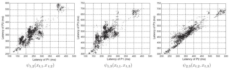
Illustration of the nonlinear distribution within pairwise potentials constructed from 3000 ICP pulses randomly extracted from the training dataset. For better visualization, only the latency dimensions is shown.

Practically, solving Eq. (3) exactly is not feasible because the conditional dependencies between different peaks, and the likelihood functions in the model are non-Gaussian ones. For these reasons, we propose to use a graphical model formalism (Section 2.3) to represent this problem, and a nonparametric Bayesian method to perform the peak tracking (Section 2.4).

2.3. Probabilistic tracking framework

The graphical model used in our tracking framework defines relations between pairs of nodes only. It is usually referred to as pairwise Markov random field (PMRF) in the literature.

As illustrated in Fig. 3(a), states x_t,i ∈ x and observations y_t,i ∈ y are represented in the graphical model by white, and shaded nodes, respectively. Edges represent dependencies between states, and possibly observations, by two types of functions: observation potentials ϕ(x_t,i, y_t,i) that are the equivalent of the likelihood part p(y_t,i∣x_t,i), and compatibility potentials ψ_ij(x_t,i, x_t,j) that embed the conditional parts p(x_t,i∣x_t,j), p(x_t,j∣x_t,i) of the Bayesian formulation and can be used by conditioning them in either directions during inference. By introducing compatibility potentials between states of the same peak at successive times ψ(x_t,i, x_t−1,i), that we name temporal potentials, the PMRF becomes a dynamic Markov model, as illustrated in Fig. 3(b).

Fig. 3.

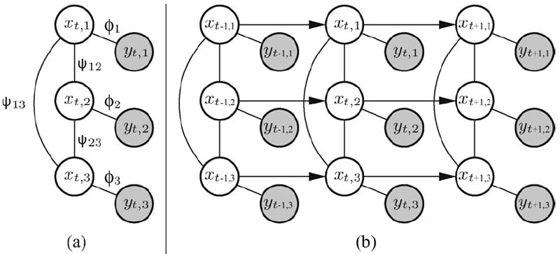
The graphical model represents the dependence through pairwise potentials (ψ₁₂, ψ₁₃, ψ₂₃) between hidden nodes (x₁, x₂, x₃), and likelihood functions (ϕ₁, ϕ₂, ϕ₃) between hidden and observable nodes (y₁, y₂, y₃) (a). By introducing temporal potentials between sucessive nodes (b), the graphical model becomes dynamic and allows for tracking ICP peaks in real time.

2.3.1. Observation model

An observation y_t,i represents the information about the position of the ith peak that is directly extracted from a raw ICP pulse at time t via a peak detector.

More formally, an observation y_t,i ∈ {ℝ² ∪ Ø} in our model corresponds to the position of the ith peak, in terms of latency and ICP elevation, that was produced by a peak detector at time t. Our framework uses MOCAIP [13] as peak detector but any other peak detection technique, such that the one based on regression models [22], could in principle be used within our model. After being trained on a set of manually annotated pulses, the peak detector can detect the position of the peaks in newly acquired ICP pulses. Due to noise and artifacts present in the pulse, the detector might not be able to detect a peak in the current pulse. In such cases, the detector assigns the empty set Ø to the observation y_t,i of the peak.

Observations y_t,i are linked probabilistically to their state x_t,i through an observation potential ϕ(x_t,i, y_t,i). Eq. (4) formalizes the integration of the observation within a Gaussian model,

$$\varphi (x_{t,i},y_{t,i})=\{\begin{array}{ll}\exp (-{\alpha }^{-1}{|y_{t,i}-x_{t,i}|}^2),& \mathrm{if}(y_{t,i}\ne \varnothing )\\ {\mathrm{\lambda }}_i,& \mathrm{if}(y_{t,i}\ne \varnothing )\end{array}$$ (4)

where α is a smoothing parameter, and λ_i is a constant factor that accounts for missing peaks by the detector.

2.3.2. Compatibility and temporal potentials

Temporal potentials ψ(x_t−1,i, x_t,i) define the relationship between two successive states of a peak. They are defined as a Gaussian difference between their arguments,

$$\psi (x_{t-1,i},x_{t,i})=\exp \left(\frac{-{|x_{t-1,i}-x_{t,i}|}^2}{{\sigma }_t^2}\right)$$ (5)

where the standard deviation σ_t of the model was previously estimated using maximum likelihood (ML) on training data.

Compatibility potentials ψ_i,j(x_t,i, x_t,j), however, are not expected to follow a Gaussian distribution. An essential property of our framework is to be able to represent and to exploit the nonlinear relation that exists between ICP peaks. To do so, each potential is represented by a KDE ψ_i,j(x_t,i, x_t,j) = f̂ (x_ij; Θ) (Eq. (6)) that is constructed by collecting a total of N_c co-ocurring ICP peak positions {p_i, p_j}_1…Nc across the training set.

$$\widehat{f}(x_{\mathit{ij}};\Theta )=\frac{1}{N_c}\sum _{k=1}^{N_c}G(x_{\mathit{ij}};\{p_i^k,p_j^k\},{\mathit{\sum }}_{\mathit{ij}})$$ (6)

where $G(x_{\mathit{ij}};\{p_i^k,p_j^k\},{\mathit{\sum }}_{\mathit{ij}})$ is a Gaussian kernel centered at $\{p_i^k,p_j^k\}$ with standard deviation Σ_ij which is common to all the components k. Θ = {{P_i, P_j}_1…Nc, Σ_ij} denotes the parameter set of the KDE and the two observed peaks of a component are bidimensional and defined in terms of their latency and ICP elevation $p_i^k=\{{\mu }_i,v_i\}$, and $p_j^k=\{{\mu }_j,v_j\}$.

2.4. Tracking ICP morphology using nonparametric Bayesian inference

Detecting peaks in an ICP pulse at time t amounts to estimating p(x_t∣y_{1…t}), the posterior belief associated with the states x_t = {x_t,1, x_t,2, x_t,3} given all observations y_{1…t} = {y_{1…t},1, y_{1…t},2, y_{1…t},3} accumulated so far. Thus, peak detection is achieved through inference in our graphical model. One way to do this efficiently is to use NBP [16]. It is a message passing algorithm for graphical models that generalizes particle filtering and belief propagation (BP). Messages are repeatedly exchanged between nodes to perform inference. Following the notation of BP, a message m_ij sent from node i to j is written,¹

$$m_{i,j}(x_j)\leftarrow \mathit{\int }{\psi }_{i,j}(x_i,x_j){\varphi }_i(x_i,y_i)\prod _{k\in N_{i\backslash j}}{m}_{k,i}(x_i){\mathit{dx}}_i$$ (7)

where N_i\j is the set of neighbors of state i where j is excluded, ψ_i,j(x_i, x_j) is the pairwise potential between nodes i, j, and ϕ_i(x_i, y_i) is the observation potential. Each message m_i,j(x_j) as well as each node x_i ∈ x distribution is represented through a multivariate KDE that is defined as,

$$\widehat{f}(x_i;\Theta )=\frac{1}{N_a}\sum _{k=1}^{N_a}{w}_i^{k}G(x_i;s_i^k,{\mathit{\sum }}_i^k)$$ (8)

where $G(x_i;s_i^k,{\mathit{\sum }}_i^k)$ is a Gaussian kernel centered at point $s_i^k\in {ℝ}^2$ that represents the position of the peak, $w_i^k$ is the weight, ${\mathit{\sum }}_i^k$ is a smoothing matrix (i.e. bandwidth), and N_a is the number of particles in the KDE.

To compute an outgoing message m_i,j(x_j) (Algorithm 1), NBP requires the pairwise potential Ψ_i,j(x_i, x_j), which represents the joint distribution between the nodes, to be conditioned on the source state x_i. This task is achieved by sampling N_a particles $s_j^k\leftarrow {\psi }_{i,j}(x_i=s_i^k,x_j)$ from the potential and then selecting a kernel bandwidth ${\mathit{\sum }}_i^k$ to complete the kernel density estimate. A common way to compute the bandwidth is to use the k nearest neighbors, where an empirical choice for the integer k is $k\approx N_a^{1/2}$.

After any iteration of message exchanges, each state can compute an approximation p̂(x_i∣y_{1…t}), called belief, to the marginal distribution p(x_i∣y_{1…t}) by combining the incoming messages with the local observation:

$$\widehat{p}(x_i\mid y_{\{1\dots t\}})\leftarrow {\varphi }_i(x_i,y_i)\prod _{k\in N_i}{m}_{k,i}(x_i)$$ (9)

The estimation of messages (Eq. (7)) and beliefs (Eq. (9)) requires the computation of a product of Gaussian kernel densities. The product of N_q Gaussian densities [16] of mean s_1…Nq and variance Σ_1…Nq is a Gaussian of mean s̄ and variance Σ̄ given by,

$$\overline{s}=\overline{\sum }\left(\sum _{k=1}^{N_q}{\mathit{\sum }}_k^{-1}{s}_k\right)\overline{\sum }={\left(\sum _{k=1}^{N_q}{\mathit{\sum }}_k^{-1}\right)}^{-1}$$ (10)

The weight w̄ associated with component G(x_i; s̄, Σ̄) of the product is,

$$\overline{w}=\frac{{\prod }_{k=1}^{N_q}{w}_{k}G(x_i;s_k,{\mathit{\sum }}_k)}{G\left(x_i;\overline{s},\overline{\sum }\right)}.$$ (11)

For tree-structured graphs, the beliefs (Eq. (9)) will converge to the exact solution p(x_i∣y_{1…t}). On graphs with cycles, NBP is not guaranteed to converge. In practice, as it has been observed in previous works [16], the algorithm exhibits satisfactory performance.

2.5. Validation procedure

Our tracking framework is evaluated on real and artificially created sequences of ICP pulses. While real ICP sequences are useful to evaluate how the framework performs on ICP recordings acquired under clinical conditions, artificially created sequences allow to evaluate the robustness of the method on pre-defined dynamics of waveform changes and noise. Real ICP sequences are extracted from our dataset by randomly selecting 30 min of consecutive recording for each patient. Artificial ICP sequences are generated by randomly selecting a raw ICP pulse from each patient in our dataset and by applying a given dynamic to it for a duration of 30 min, which amounts approximately to 2800 pulses. The temporal dynamic applied follows either: (a) a sinusoidal trend, or (b) a phase multiplication, as described below.

1. Sinusoidal temporal dynamic: Let S_i denote a raw ICP pulse extracted randomly from a recording, an artificial sequence Q_t=1…N of N pulses is generated by applying a sinusoidal trend in latency to the pulse S_i. This amounts to shifting the pulse (Eq. (12)) using a series that follows a sinusoidal dynamic.

$$Q_t=\mathit{circshift}(S_i,t)\mid t=1\dots N$$ (12)

where N is the total number of pulses in the sequence, and the circular shift function Γ = circshift(S_i, t) is defined as,

$$\Gamma (a)=S_i((a-h_t)\%s)+\xi \mid a=1\dots s$$ (13)

where s is the length of a pulse, % denotes the modulo operator that finds the remainder of the division, h_t is the amount of shifts for the tth pulse of the sequence and follows a sinusoidal dynamic,

$$h_t=\sin \left(\frac{2\pi t}{N}\right)$$ (14)

The sinusoidal ICP sequence, which is shown at the top of Fig. 4 by a green curve, is perturbed by a Gaussian noise ξ which has a variance of 20 ms.

Fig. 4.

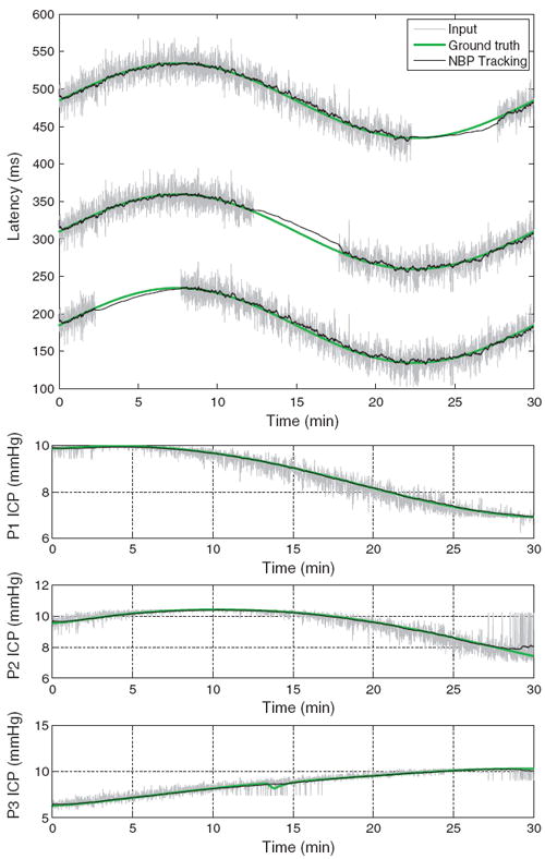
Results of the NBP tracking (black) on an artificial sequence of ICP pulses affected by a sinusoidal dynamic (top), and phase shifting (bottom three plots). Latency dimension is reported for the sinusoidal dynamic, while ICP elevation is shown for the phase shifting. In both sequences, the predictions of the tracking algorithm closely follow the groundtruth (green). (For interpretation of the references to color in this figure legend, the reader is referred to the web version of the article.)

In addition, to make the problem more challenging, we purposely blanked the input for a duration of about 8 min for each peak. We hypothesize that the tracking will be able to recover the latency of the peaks, through the pairwise potentials, even if the evidence in the current pulse is not available for a given peak.

1. Phase multiplication dynamic: The second type of artificial sequence is produced from a raw ICP pulse S_i by multiplying the phase of the pulse by a factor that varies linearly between [0.5,1.5]. The phase of the pulse is obtained using a discrete Fourier transform a = fft(S_i) computed with a fast Fourier transform algorithm. After multiplying the phase with a factor proportional to the current time within the artificial sequence, the pulse is projected back using an inverse Fourier transform ϒ = ifft(a*), thus producing an artificially altered pulse of the sequence.

The tracking algorithm predicts state estimates x̂_t,1, x̂_t,2, x̂_t,3 of the three peaks in terms of their latency and ICP elevation at each time t, so that x̂_t,1 = {μ̂_t,1, ν_t,1}, x̂_t,2 = {μ̂_t,2, v̂_t,2}, x̂_t,3 = {μ̂_t,3, v̂_t,3}. For the sinusoidal dynamic, the predicted latency {μ̂_t,1, μ̂_t,2, μ̂_t,3} is evaluated quantitatively against the actual artificial trend minus noise ξ (Eq. (12)), which corresponds to the groundtruth {μ₁, μ₂, μ₃}. The average prediction error ē_l is reported in milliseconds (ms) between the actual position of the peaks and the prediction,

$$\{{\overline{e}}_{{\mu }_1},{\overline{e}}_{{\mu }_2},{\overline{e}}_{{\mu }_3}\}=\frac{1}{n}\sum _{t=1}^N|\{{\widehat{\mu }}_{t,1},{\widehat{\mu }}_{t,2},{\widehat{\mu }}_{t,3}\}-\{{\mu }_{t,1},{\mu }_{t,2},{\mu }_{t,3}\}|$$ (15)

where N is the total number of pulses in the artificial sequence, and ē_μ1 denotes the prediction error for the first peak, and ē_μl = (ē_μ1 + ē_μ2 + ē_μ3)/3 is the average latency error for the three peaks.

In contrast with the sinusoidal dynamic that only affects the latency of the peaks, the phase multiplication trend has its main effect on the pressure elevation of the peaks. The prediction error of the tracking algorithm is therefore measured on the phase multiplication trend by comparing the predicted peak elevations {v̄_t,1, v̄_t,2, v̄_t,3} of the tracking algorithm against the groundtruth {v_t,1, v_t,2, v_t,3} that was obtained by manual annotation. The average prediction error ē_p is reported in millimeter of mercury (mmHg) between the actual elevation of the peaks and the prediction,

$$\{{\overline{e}}_{v_1},{\overline{e}}_{v_2},{\overline{e}}_{v_3}\}=\frac{1}{n}\sum _{t=1}^N|\{{\widehat{v}}_{t,1},{\widehat{v}}_{t,2},{\widehat{v}}_{t,3}\}-\{v_{t,1},v_{t,2},v_{t,3}\}|$$ (16)

where N is the total number of pulses, and ē_v1 denotes the prediction error for the first peak, and ē_p = (ē_v1 + ē_v2 + ē_v3)/3 is the average pressure error for the three peaks.

For evaluation on clinically recorded ICP sequence, we run the tracking algorithm on 30 min segments randomly chosen within the full recording. The model is trained on 20 representative patients, and predictions, in terms of latency and ICP, are evaluated on the remaining 108 patients. It is important to notice that the latencies and elevations are estimated jointly, and in real-time, using the result of MOCAIP peak detector applied on raw ICP pulses as input y. We compare the real-time prediction obtained by the tracking framework with post-processing results obtained by MOCAIP on dominant pulses. These dominant pulses are computed over a segment of ICP recording (of length comprises between 1 and 180 s) and are expected to be robust to noise. In addition, the tracking is also performed on a 30 min ICP recording of a patient who was administered Versed (Midozalam) intravenously at 6 mg per hour starting after 5 min on the recording. This drug is usually applied to TBI patients to decrease their mean ICP. We use our tracking algorithm to evaluate the impact of the drug on the patient ICP. Finally, we evaluate the robustness of the tracking algorithm against missing peaks. Because the real ICP is not known, another reference signal has to be used as ground truth. For this experiment, it is set to the estimated output of the tracking algorithm where all the individual input pulses are used (100%). It is reasonable to expect that the tracking results on all the available input peaks will lead to a more reliable estimation of the ICP morphology in comparison to estimations made from missing input peaks. To measure this impact, we repeatidly run the tracking algorithm by keeping a subset of 90%; 70%; 50%; 30%; 10% of the input peaks. Peaks are selected randomly and in an independent fashion for each peak so that the first peak may be discarded on one pulse but the second and third may still be present. The average distance and standard deviation to the results obtained with the full set of peaks (100%) are reported as a measure of performance.

3. Results

Fig. 4 illustrates the estimated latency (black), the groundtruth (green), and the input² (gray) for the three peaks in presence of a sinusoidal temporal dynamic. The proposed method can recover the intrinsic trend despite the noise, and missing inputs. For this experiment, it obtains an average prediction error in latency of 8.09 ± 2.0 ms, 6.90 ± 1.7 ms, and 7.46 ± 2.1 ms for the first, second, and third peak, respectively. In comparison, a pulse by pulse detection using MOCAIP peak detector, which is affected by transient perturbations, has average errors of 11.88 ± 7.1 ms, 11.80 ± 7.0 ms, and 11.76 ± 7.0 ms. The probabilistic model, and the use of temporal information clearly helps to produce a better estimate of the peaks latency on these artificial data. For the second experiment, we report in the bottom of Fig. 4 the estimated peak elevation under a phase multiplication dynamic of the ICP pulse. Similarly to the results observed for the sinusoidal dynamic on the latency, the tracking algorithm (black) is able to give estimates that closely follow the groundtruth (green). Average error in ICP elevation for the three peaks are 0.04 ± 0.02 mmHg, 0.09 ± 0.06 mmHg, 0.08 ± 0.04 mmHg for the tracking, and 0.23 ± 0.18 mmHg, 0.32 ± 0.27 mmHg, 0.33 ± 0.23 mmHg for the pulse by pulse MOCAIP.

Fig. 5 illustrates the predicted latency and ICP elevation for MOCAIP (left) and for the proposed tracking method (right) on a 30-min ICP recording. To overcome noise, MOCAIP may extract a cleaner dominant pulse by applying a hierarchical clustering on a series of consecutive ICP pulses. The left column illustrates how the sequence length, used in MOCAIP to extract of the dominant pulse, impacts of the positions of the peaks. The duration varies from less than 1 to 180 s. Because a longer duration means that more ICP pulses are used to compute the dominant pulse, it generally leads to a smoother estimate of the peak locations. For example, we can observe that the blue curve, corresponding to an interval of 180 s, does not seem to be affected by noise in the top left plot, while the predictions on raw pulses (red) are not reliable and exhibit a lot of variations. In MOCAIP, the length of the sequence chosen is critical and reflects a tradeoff between invariance to noise and sensitivity to quick changes. The proposed tracking framework, shown on the right, can capture rapid changes in elevation and latency while remaining robust to transient noise. In addition, while MOCAIP is usually applied as a post-processing tool due the computational complexity of the hierarchical clustering, the developped framework can be applied in real time.

Fig. 5.

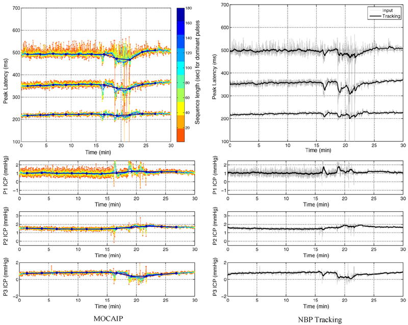
Peak latency (top) and ICP elevation (bottom) estimated on real ICP sequences by MOCAIP (left) and the NBP tracking algorithm (right). For MOCAIP, the effect of the length of the sequence of raw ICP pulse used to extract a dominant pulse is depicted by different colors (1 s (red) to 180 s (blue)). The predictions of the tracking are obtained in real-time and are robust to transient perturbations that frequently occur during the ICP signal recording. (For interpretation of the references to color in this figure legend, the reader is referred to the web version of the article.)

In Fig. 6, we present an average ICP pulse computed from 10 successive raw pulses. The predicted location of the three peaks for the proposed tracking algorithm are compared to the ones obtained by using MOCAIP. Because it does not exploit temporal correlation, MOCAIP detector leads to inconsistent predictions between the second and the third peak. In contrast, the tracking algorithm gives a more robust and precise location of the peaks.

Fig. 6.

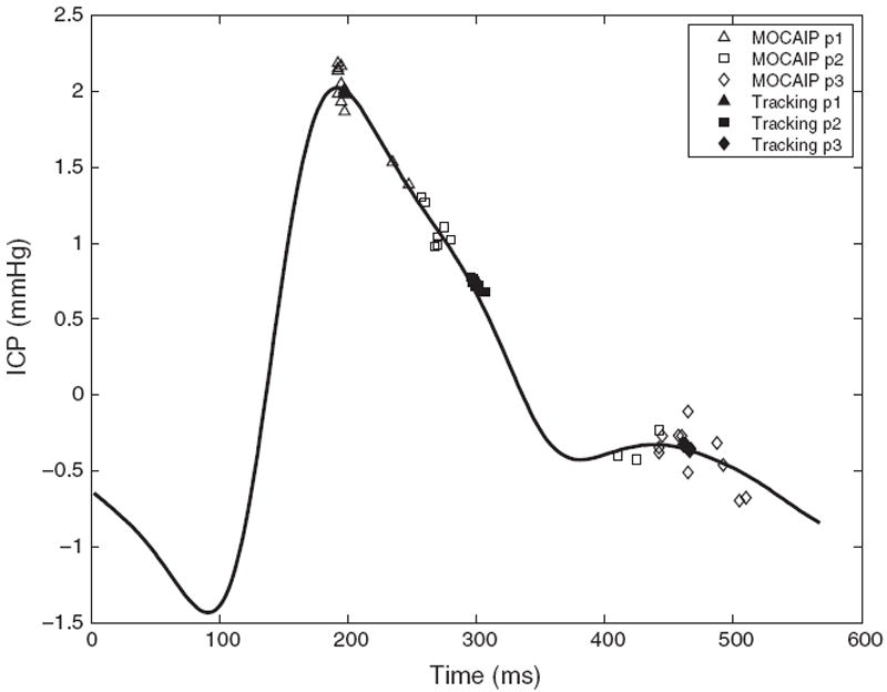
Illustration of an average ICP pulse computed from 10 successive raw pulses. Predicted peak locations (p1, p2, and p3) are shown for the proposed tracking algorithm (black), and using a peak detector (MOCAIP) that does not exploit temporal correlation. While the raw peak detector leads to inconsistent predictions between the second and the third peak, the tracking algorithm gives a more robust and precise location of the peaks.

Fig. 7 shows the tracking results for the three peaks on a patient administered with Versed after approximately 5 min. This drug aims at decreasing the mean ICP. Our framework is particularly useful to provide insight to the changes in waveform morphology in a continuous fashion. While the latency of the peaks does not change significantly, their ICP elevation exhibits different kind of changes. The first peak increases, the third decreases, and the second peak remains stable. The observation potential of the tracking framework corresponds to the detected peak obtained by MOCAIP on raw pulses. Fig. 7 also shows that the confidence given to the observation, that is adjusted by a standard deviation parameter (α in Eq. (4)), impacts on the prediction. A larger standard deviation means that less importance is given to the current pulse, and thus leads to smoother variations (red, right column). Fig. 8 shows the corresponding changes in morphology, before and after 5 min administration of Versed. Table 1 reports the results of the tracking algorithm across different percentages (10%; 30%; 50%;70%; 90%) of peaks used as input to the algorithm. When only 10% of the peaks are used as input, the error reaches an error rates of 11.14 ± 11.3 ms, 14.71 ± 14.2 ms, 14.80 ± 13.7 ms for the latency and 0.140 ± 0.12 mmHg, 0.094 ± 0.08 mmHg, 0.104 ± 0.09 mmHg for the ICP of the peaks p1, p2, p3, respectively. Note that these performances have limitations in the sense that they are compared to the results of the tracking using all the peaks (100%), and may also be linked to the sampling rate. These results were produced with a sampling rate of 400 Hz for the recorded ICP signal, performances may rapidly deteriorate with lower sampling rates.

Fig. 7.

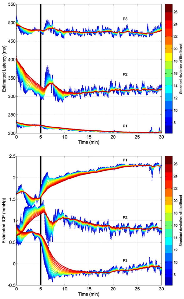
Real-time joint tracking of peak latency estimation (top) and ICP elevation (bottom) for the three peaks on a patient administrated with Versed after 5 min. The effect of the smoothing parameter α_g, which controls the confidence of evidence extracted from the current pulse, is shown by different colors. While a high confidence (blue) help to capture quick changes, less confidence (red) tends to smooth the estimation and to obtain more robustness to transient perturbations. (For interpretation of the references to color in this figure legend, the reader is referred to the web version of the article.)

Fig. 8.

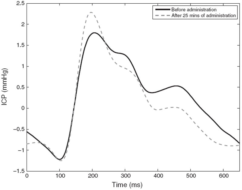
Effect of intravenous administration of Versed on the ICP waveform morphology.

Table 1.

Average error and standard deviation of the estimated latency and ICP elevation of the three peaks by the tracking algorithm across different percentages of missing input peaks.

	Pct of input peaks used/Avg error
	10%	30%	50%	70%	90%
Latency
p1 (ms)	11.14 ± 11.3	7.48 ± 7.9	5.14 ± 5.8	3.17 ± 3.6	1.40 ± 1.9
p2 (ms)	14.71 ± 14.2	9.11 ± 8.9	6.33 ± 6.6	4.08 ± 4.4	1.84 ± 2.4
p3 (ms)	14.80 ± 13.7	9.69 ± 9.1	6.71 ± 6.8	4.26 ± 4.3	1.99 ± 2.3
ICP
p1 (mmHg)	0.140 ± 0.12	0.086 ± 0.07	0.058 ± 0.05	0.036 ± 0.03	0.016 ± 0.02
p2 (mmHg)	0.094 ± 0.08	0.060 ± 0.05	0.041 ± 0.03	0.026 ± 0.02	0.012 ± 0.01
p3 (mmHg)	0.104 ± 0.09	0.066 ± 0.06	0.044 ± 0.04	0.029 ± 0.02	0.013 ± 0.01

4. Discussion

The present work has significantly furthered a series of efforts from our group towards the next generation of ICP monitoring in terms of providing a comprehensive and quantitative characterization of morphology of an ICP pulse [13,22]. Such a technical capability would provide far more information to clinicians than the average value of ICP currently supplied by monitoring devices. The tracking algorithm, as proposed and evaluated in this present work, has increased the temporal resolution of detecting ICP pulse morphological changes from the minute-level to the beat-level. More importantly, the algorithm relies on NBP inference, which has a strong theoretical basis and has been proven successful in many other fields requiring solution of a tracking problem [25,26].

The proposed tracking algorithm explicitly models, in a probabilistic fashion, two types of correlative relations: (1) the correlation of peak characteristics between successive ICP pulses; (2) the correlation among peaks of the same pulse. The tracking algorithm, in essence, benefits from such an explicit model while previous peak recognition methods [13,22] failed to capitalize on these two types of correlations. Although the loopy topology of the graphical model adopted here prevents us from achieving a theoretically optimal solution using the message passing algorithm, our results indicate that the algorithm works quite well in practice as experienced by other existing publications [25,27] in different fields. It remains interesting to see the effect of removing the loop in the model as it might require additional nodes but would enable optimal inference using the message passing algorithm.

The quantitative experiments on artificially created sequences of ICP pulses demonstrated the effectiveness of the tracking algorithm. Known trends in the signal were tracked accurately. More impressively, it has been demonstrated that it is still feasible to recover missing peak information by exploiting the correlation among peaks of the same pulse. This has a significant practical implication because it is not rare in practice to be unable to recognize ICP peaks when we consider only a single dominant pulse. For instance, as it has been reported in a previous study [22] on a database of 13,611 dominant pulses, 1717 had missing p1, 265 had missing p2, and 34 had missing p3. In practice, the peaks tend to dissapear gradually. Even thought a peak might not be visible in the current pulse, it is still desirable to be able to extract its plausible location. Even when a peak is not clearly visible, the tracking algorithm can estimate its most likely position given the past pulses and the context (position of the two other peaks). Being able to summarize the ICP waveform morphology as a fixed size vector even when peaks cannot be observed is a key property of the tracking framework that should lead to improved ICP morphology analysis.

When applied to real ICP pulses, the algorithm confirms its good performances and it is able to reliably estimate the ICP elevation and latency of the three peaks in a beat-by-beat fashion. To the best of our knowledge, this is the first successful attempt to track peaks of ICP signals at such a temporal resolution. Although additional clinical research is needed to demonstrate the impact of this tracking algorithm, it can be fairly predicted that leveraging such a high temporal resolution will surely improve the timeliness of detecting pulse morphological changes and offer innovative solutions in practicing the advocated next generation ICP monitoring in a challenging clinical environment.

Algorithm 1. NBP update of an outgoing nonparametric message Given messages $m_{\mathit{ij}}(x_j)={\left\{s_{\mathit{ij}}^k,{\mathit{\sum }}_{\mathit{ij}}^k,w_{\mathit{ij}}^k\right\}}_{k=1}^{N_a}$ received from nodes i ∈ N_j\u

1. //Compute Incoming Message Product and Draw M samples

   $${\{{\overline{s}}_j^k,{\overline{\mathrm{\sum }}}_j^k,{\overline{w}}_j^k\}}_{a=1}^{N_a}\leftarrow {\varphi }_j(x_j,y_j){\mathrm{\Pi }}_{i\in N(j)\backslash u}{m}_{\mathit{ij}}(x_j)$$

2. //Map the Pairwise Potential $\{s_{\mathit{ju}}^k,w_{\mathit{ju}}^k\}=\mathrm{apply}\{{\overline{s}}_j^k,{\overline{w}}_j^k\}$ on the potential ψ_j,u

3. //Adjust the Kernel bandwidth

   $$\forall i\in [1\dots N_a],{\mathit{\sum }}_{\mathit{ju}}^k=\mathit{kde}(x_{\mathit{ju}},k)$$
4. Compose the Outgoing message

   $$m_{\mathit{ju}}(x_u)={\{x_{\mathit{ju}}^k,{\mathit{\sum }}_{\mathit{ju}}^k,w_{\mathit{ju}}^k\}}_{k=1}^{N_a}$$

References

- 1.Piper I. Head injury: pathophysiology and management of severe closed injury. chapter 6 Chapman & Hall Medical; 1997. Intracranial pressure and elastance; pp. 101–20. [Google Scholar]
- 2.Balestreri M, Czosnyka M, Steiner L, Schmidt E, Smielewski P, Matta B, et al. Intracranial hypertension: what additional information can be derived from ICP waveform after head injury? Acta Neurochir (Wien) 2004;146(2):131–41. doi: 10.1007/s00701-003-0187-y. [DOI] [PubMed] [Google Scholar]
- 3.Czosnyka M, Guazzo E, Whitehouse M, Smielewski P, Czosnyka Z, Kirkpatrick P, et al. Significance of intracranial pressure waveform analysis after head injury. Acta Neurochir (Wien) 1996;138(5):531–41. doi: 10.1007/BF01411173. [DOI] [PubMed] [Google Scholar]
- 4.Contant CF, Robertson CS, Crouch J, Gopinath SP, Narayan RK, Grossman RG. Intracranial pressure waveform indices in transient and refractory intracranial hypertension. J Neurosci Methods. 1995;57(l):15–25. doi: 10.1016/0165-0270(94)00106-q. [DOI] [PubMed] [Google Scholar]
- 5.Takizawa H, Gabra-Sanders T, Miller JD. Changes in the cerebrospinal fluid pulse wave spectrum associated with raised intracranial pressure. Neuro-surgery. 1987;20(3):355–61. doi: 10.1227/00006123-198703000-00001. [DOI] [PubMed] [Google Scholar]
- 6.Cardoso ER, Reddy K, Bose D. Effect of subarachnoid hemorrhage on intracranial pulse waves in cats. J Neurosurg. 1988;69(5):712–8. doi: 10.3171/jns.1988.69.5.0712. [DOI] [PubMed] [Google Scholar]
- 7.Cardoso ER, Rowan JO, Galbraith S. Analysis of the cerebrospinal fluid pulse wave in intracranial pressure. J Neurosurg. 1983;59(5):817–21. doi: 10.3171/jns.1983.59.5.0817. [DOI] [PubMed] [Google Scholar]
- 8.Portnoy HD, Chopp M. Cerebrospinal fluid pulse wave form analysis during hypercapnia and hypoxia. Neurosurgery. 1981;9(1):14–27. doi: 10.1227/00006123-198107000-00004. [DOI] [PubMed] [Google Scholar]
- 9.Chopp M, Portnoy HD. Systems analysis of intracranial pressure, comparison with volume–pressure test and csf-pulse amplitude analysis. J Neurosurg. 1980;53(4):516–27. doi: 10.3171/jns.1980.53.4.0516. [DOI] [PubMed] [Google Scholar]
- 10.Hu X, Glenn T, Scalzo F, Bergsneider M, Sarkiss C, Martin N, et al. Intracranial pressure pulse morphological features improved detection of decreased cerebral blood flow. Physiol Meas. 2010;31:679–95. doi: 10.1088/0967-3334/31/5/006. [DOI] [PMC free article] [PubMed] [Google Scholar]
- 11.Hu X, Xu P, Asgari S, Vespa P, Bergsneider M. Forecasting icp elevation based on prescient changes of intracranial pressure waveform morphology. IEEE Trans Biomed Eng. 2010;57(5):1070–8. doi: 10.1109/TBME.2009.2037607. [DOI] [PMC free article] [PubMed] [Google Scholar]
- 12.Aboy M, McNames J, Thong T, Tsunami D, Ellenby M, Goldstein B. An automatic beat detection algorithm for pressure signals. IEEE Trans Biomed Eng. 2005;52(10):1662–70. doi: 10.1109/TBME.2005.855725. [DOI] [PubMed] [Google Scholar]
- 13.Hu X, Xu P, Scalzo F, Vespa P, Bergsneider M. Morphological clustering and analysis of continuous intracranial pressure. IEEE Trans Biomed Eng. 2009;56(3):696–705. doi: 10.1109/TBME.2008.2008636. [DOI] [PMC free article] [PubMed] [Google Scholar]
- 14.Eide P. A new method for processing of continuous intracranial pressure signals. Med Eng Phys. 2006;28(6):579–87. doi: 10.1016/j.medengphy.2005.09.008. [DOI] [PubMed] [Google Scholar]
- 15.Ellis T, McNames J, Aboy M. Pulse morphology visualization and analysis with applications in cardiovascular pressure signals. IEEE Trans Biomed Eng. 2007;54(9):1552–9. doi: 10.1109/TBME.2007.892918. [DOI] [PubMed] [Google Scholar]
- 16.Sudderth EB, Ihler AT, Freeman WT, Willsky AS. Nonparametric belief propagation. IEEE computer society conference on Computer Vision and Pattern Recognition (CVPR) 2003;1:605–12. [Google Scholar]
- 17.Eide PK. Comparison of simultaneous continuous intracranial pressure (ICP) signals from ICP sensors placed within the brain parenchyma and the epidural space. Med Eng Phys. 2008;30:34–40. doi: 10.1016/j.medengphy.2007.01.005. [DOI] [PubMed] [Google Scholar]
- 18.Eide PK, Saehle T. Is ventriculomegaly in idiopathic normal pressure hydrocephalus associated with a transmantle gradient in pulsatile intracranial pressure? Acta Neurochir (Wien) 2010;152:989–95. doi: 10.1007/s00701-010-0605-x. [DOI] [PubMed] [Google Scholar]
- 19.Wagshul ME, Eide PK, Madsen JR. The pulsating brain: a review of experimental and clinical studies of intracranial pulsatility. Fluids Barriers CNS. 2011;8:5. doi: 10.1186/2045-8118-8-5. [DOI] [PMC free article] [PubMed] [Google Scholar]
- 20.Hu X, Xu P, Lee D, Vespa P, Bergsneider M. An algorithm of extracting intracranial pressure latency relative to electrocardiogram r wave. Physiol Meas. 2008;29:459–71. doi: 10.1088/0967-3334/29/4/004. [DOI] [PMC free article] [PubMed] [Google Scholar]
- 21.Afonso VX, Tompkins WJ, Nguyen TQ, Luo S. Ecg beat detection using filter banks. IEEE Trans Biomed Eng. 1999;46(2):192–202. doi: 10.1109/10.740882. [DOI] [PubMed] [Google Scholar]
- 22.Scalzo F, Xu P, Asgari S, Bergsneider M, Hu X. Regression analysis for peak designation in pulsatile pressure signals. Med Biol Eng Comput. 2009;47(9):967–77. doi: 10.1007/s11517-009-0505-5. [DOI] [PMC free article] [PubMed] [Google Scholar]
- 23.Scalzo F, Asgari S, Kim S, Bergsneider M, Hu X. Robust peak recognition in intracranial pressure signals. Biomed Eng Online. 2010;9:61. doi: 10.1186/1475-925X-9-61. [DOI] [PMC free article] [PubMed] [Google Scholar]
- 24.Kaufman L, Rousseeuw PJ. Wiley series in probability and mathematical statistics. Hoboken, NJ: Wiley; 2005. Finding groups in data: an introduction to cluster analysis. [Google Scholar]
- 25.Sudderth EB, Mandel MI, Freeman WT, Willsky AS. Visual hand tracking using nonparametric belief propagation. IEEE Computer Society Conference on Computer Vision and Pattern Recognition Workshop (CVPRW) 2004;1:189. [Google Scholar]
- 26.Bernier O, Cheung-Mon-Chan P, Bouguet A. Fast nonparametric belief propagation for real-time stereo articulated body tracking. Comput Vis Image Underst. 2009;113(1):29–47. [Google Scholar]
- 27.Scalzo F, Piater JH. Adaptive patch features for object class recognition with learned hierarchical models. IEEE conference on Computer Vision and Pattern Recognition Workshop (CVPRW) 2007;1:1–8. [Google Scholar]