Virtual Cell: computational tools for modeling in cell biology

Abstract

The Virtual Cell (VCell) is a general computational framework for modeling physico-chemical and electrophysiological processes in living cells. Developed by the National Resource for Cell Analysis and Modeling at the University of Connecticut Health Center, it provides automated tools for simulating a wide range of cellular phenomena in space and time, both deterministically and stochastically. These computational tools allow one to couple electrophysiology and reaction kinetics with transport mechanisms, such as diffusion and directed transport, and map them onto spatial domains of various shapes, including irregular three-dimensional geometries derived from experimental images. In this article, we review new robust computational tools recently deployed in VCell for treating spatially resolved models.

1. Introduction

The Virtual Cell (VCell) is a problem-solving environment designed for cell biologists and theorists to model and simulate processes in living cells (1-9). There are two workspaces in VCell: the BioModel workspace and the math workspace. In the BioModel workspace, a user enters a model through a graphical user interface, much like drawing a cartoon of a model. The design of the BioModel interface allows applying various modeling and computational techniques to a given collection of mechanisms comprising a biological model. This is done by creating multiple applications using the same model. For example, the same set of mechanisms can be simulated deterministically or stochastically. If diffusion is fast, one can assume the cellular compartments to be well-stirred and run compartmental simulations which do not resolve geometry. Alternatively, for cases where concentration gradients need to be captured, VCell provides tools for running spatial simulations in which the mechanisms are mapped onto geometries that are topologically consistent with the modeling assumptions. The geometries used in simulations can be one- two- or three- dimensional and are specified analytically or inferred from experimental images. Overall, simulations in VCell can be either spatial or compartmental (nonspatial), deterministic or stochastic (tools for spatial stochastic simulations are the most recent addition to VCell; they have been developed through integration with a software package called Smoldyn (10, 11) and deployed in VCell-Beta for further testing).

In the BioModel workspace, the mathematical description of a particular application is generated automatically using appropriate conservation laws (12). This description encodes a set of mathematical equations consistent with the biological model and with additional assumptions included in the application. Given this one-to-one correspondence, the mathematical description in the VCell BioModel workspace is read-only. For editing, it must be transferred to the MathModel workspace and saved as an independent mathematical model. One can also use the MathModel workspace to create a mathematical model from scratch. Generally, the MathModel workspace provides more flexibility and freedom in the implementation of the model, but the responsibility for its physical correctness lies in this case with the user.

VCell computational tools allow a user to simulate a wide range of cellular phenomena including molecular interactions and transport in, and between, various subcellular compartments, as well as dynamics of membrane potential. These mechanisms might be interconnected and can be modeled as such. Overall, VCell can be applied to any system that is mathematically described by a reaction-diffusion-flow (advection) model in an arbitrary geometry and with arbitrary fluxes coming from, and to, cellular membranes, as well as passive and active mechanisms of cross-membrane transport.

In this article, we review new powerful computational tools and modeling capabilities that have been recently developed and deployed in VCell for simulating spatially resolved (deterministic) systems. These include: modeling of lateral diffusion of molecules in cell membranes coupled to reversible unbinding from the membrane into the cytosol (section 2), a suite of image-processing tools for generating geometries from experimental images and for incorporating experimental data in VCell simulations (section 3), and a robust spatial solver, which includes automatic time-step control and retains stability in the presence of vastly different time scales (section 4).

2. Modeling diffusion in cell membranes coupled to reaction-diffusion systems in cytosol

Problems arising in cell biology often include diffusion of molecules in the plasma membrane. This is especially true for cell signaling which is mediated in part by trans-membrane receptors that can diffuse. Computational modeling of diffusion on arbitrary surfaces is more involved than diffusion on a plane and it becomes particularly nontrivial in the case of surfaces inferred from pixilated experimental images. The problem gets even more complicated in the presence of binding interactions between cytosolic molecules and the cell membrane. In this case, the lateral diffusion in the membrane becomes mathematically coupled to the diffusion and reactions in the cytosol. The capability of modeling diffusion on a curved surface coupled to reactions and diffusion in the embedding volume is a relatively new addition to the arsenal of VCell modeling tools deployed for general use.

The representation of surfaces in VCell is “volume-based”: a user-defined geometry is placed in a rectangular box to which uniform orthogonal meshing is applied; the elementary Cartesian volumes are then assigned to compartments so that if the center of a control volume belongs to a given compartment, then the entire volume belongs to that compartment. This procedure automatically creates watertight surfaces between compartments: each such surface is a union of rectangular facets that separate neighboring control volumes which belong to different compartments.

This way of handling geometry has important practical advantages. First, the method can be automatically applied to virtually any bounded geometry, resulting in a fast procedure that requires minimal user involvement, whether the geometry is derived from images or idealized shapes, or defined analytically. Second, grid connectivity is trivial, which greatly simplifies the code. Because generation of internal surfaces is volume-based, the natural connectivity between surface and volume elements simplifies coupling between lateral diffusion of molecules in the cell membrane and a reaction-diffusion system in the embedding volume. Third, linear solvers, which are at the core of the numerical solution of equations describing a biological model, tend to converge better on regular grids than on unstructured grids and it is easier to adapt them for parallel computations on multiple processors, because of the highly regular structure of the matrices involved.

An important disadvantage of the orthogonal meshing, however, is that it results in jagged, “staircase” surfaces. That cannot be used directly for the computation of fluxes coming in or out of a compartment, because the error in such computation would not diminish as the mesh is refined (13, 14). In VCell, this problem has been solved by applying a flux-correction method (13). The method is based on an optimal approximation of vectors orthogonal to the correct surface (normals)in the vicinity of facet centers. Once the normals are known, the corrected area of surface elements are computed by projecting the facets onto a local tangential plane. It is the corrected areas that are then used for computing cross-membrane fluxes. The results obtained by this method converge to the exact flux values, provided that the approximated normals converge to the exact ones as the mesh is refined. The method of approximating normals employed in VCell, which is described in detail in (14), ensures convergence.

The problems posed by digitized surfaces are particularly challenging for modeling diffusion on curved surfaces, which requires (among other things) accurate estimates of distances along the surface. Note that even with uniform meshing of the volume, the centers of orthogonal facets comprise an unstructured mesh on the surface. Due to the lack of orthogonality of the surface mesh, resolving its connectivity becomes a nontrivial issue. In VCell, these problems are resolved by locally approximating the Laplace-Beltrami operator (which describes diffusion on curved surfaces (15)) with the Laplacian on each tangential plane (14), as illustrated by Fig. 1, left (alternative methods are described in (16, 17)). For this, a local subset of grid points is projected onto a tangential plane (this in turn requires that normals be accurately approximated, as explained above). The unstructured grid of projected points on the tangential plane is then subject to the Voronoi decomposition (18) (Fig. 1, right). The procedure automatically resolves local connectivity of a central grid point and its neighbors and defines respective distances. The Voronoi cell associated with each surface grid point is defined as the set of points that are closer to the central point than to any other neighboring grid point. The area of the Voronoi cell, its sides, and the distances between the “natural neighbors form a basis for spatial discretization of the diffusion equation on a surface that automatically preserves local mass balance (19). Because of the natural one-to-one correspondence between the surface elements and the adjacent control volumes, coupling between diffusion on the surface and diffusion in the embedding volume is also implemented in a mass-conservative manner. For this, the same surface elements that were obtained through the Voronoi decomposition of the irregular grid on the membrane, are used to compute fluxes from the volume into the surface.

Figure 1.

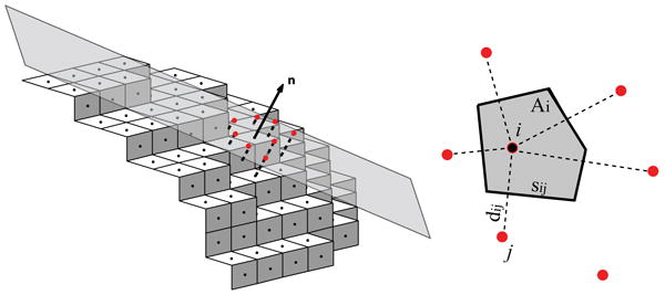
Discretization of diffusion equation on a surface: A local subset of surface grid points is projected on the tangential plane orthogonal to the outward normal vector n at point I (left) and Voronoi tessellation is then applied to projections shown in red (right). This procedure automatically determines the natural neighbors of point i, along with necessary geometric parameters: the sides s_ij area A_i of the Voronoi cell and the distances d_ij between the natural neighbors. In terms of these parameters, the spatially discretized diffusion equation takes the form, $A_{\mathrm{i}}{\partial }_t{U}_{\mathrm{i}}={\sum }_{\mathrm{j}\in \mathrm{G}(\mathrm{i})}D(U_{\mathrm{j}}-U_{\mathrm{i}})s_{\mathrm{ij}}^{\mathrm{sym}}/d_{\mathrm{ij}}^{\mathrm{sym}}$ where U_i are the concentration values at the surface grid points, D is the diffusion coefficient, $s_{\mathrm{ij}}^{\mathrm{sym}}=(s_{\mathrm{ij}}+s_{\mathrm{ij}})/2$ and $d_{\mathrm{ij}}^{\mathrm{sym}}=(d_{\mathrm{ij}}+d_{\mathrm{ij}})/2$.

The capability outlined above was recently applied to modeling experiments, in which fluorescence loss in photobleaching (FLIP) was used to measure the in vivo rates of dissociation of Rac, a G-protein regulating actin cytoskeleton, from the cell membrane (20). In these experiments, NIH3T3 fibroblasts expressing GFP-Rac were bleached continuously by a laser beam everywhere except for a small masked region at the cell periphery (Fig. 2a). Using a confocal microscope and alternating bleaching and measuring power, fluorescence loss was simultaneously recorded throughout a cell (Fig. 2b). Decay of the signal in the unbleached region was caused by dissociation of Rac from the membrane followed by diffusion in the cytosol and also by lateral diffusion of the membrane-bound Rac out of the unbleached region. A simple compartmental model built on the assumption that diffusion of Rac in the cytosol is fast pointed to a two-step procedure for retrieving the dissociation rate constant k_off from the raw data: first, fit the fluorescence decay in the bleached region with the sum of two exponential functions (the second component was likely due to inhomogeneity of light in the z-direction); second, fit the fluorescence decay in the unbleached region with the sum of three exponentials, of which two are the same as in step 1 and the third has a rate constant k_off + k_diff, where k_diff is the rate constant representing the effect of the lateral diffusion of Rac, which was estimated in a separate experiment.

Figure 2.

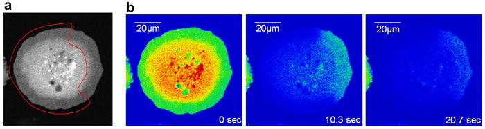
FLIP experiments with fibroblasts expressing GFP-Rac (adapted from (20)). (a) A representative cell, 30 min after replating on fibronectin. The red line delineates the photobleached area. (b) Cell in (a) at the indicated times during the photobleaching protocol.

The method of measuring k_off was derived on the assumption that diffusion of Rac in the cytosol is much faster than the processes contributing to the loss of fluorescence in the unbleached area. To assess the accuracy of this assumption, a mathematical model was constructed in VCell (14) to simulate the FLIP experiment using a realistic cell geometry obtained from experimental images (Fig. 3). The idea was to mimic the experimental protocol, collect the data in the way they were collected in real experiments, subject the simulated data to the fitting procedure described above and compare the obtained estimates of k_off with the “exact” values used in the model. These numerical experiments, performed for a wide range of parameters validated the fitting procedure overall, but also pointed to a possible underestimation of k_off (up to 30%) in cases where Rac was tightly bound to the membrane. For these cases, tight binding effectively slows down diffusion of Rac in the cytosol, and the assumption of fast diffusion underlying the fitting procedure may not be accurate.

Figure 3.

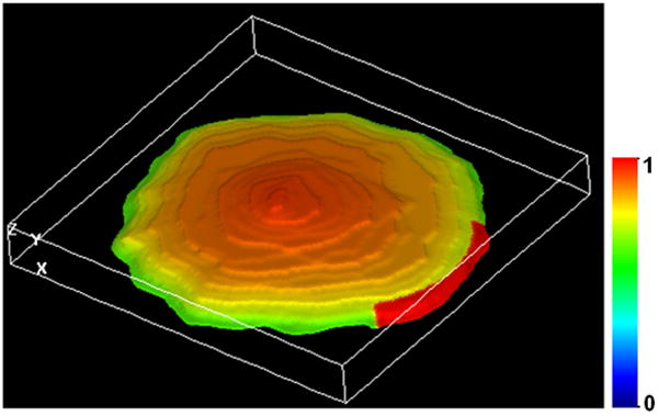
Simulation of a FLIP experiment in VCell using geometry obtained from a z-stack of confocal images (details of how image-based geometries are generated in VCell are given below in section 3). The snapshot represents distribution of the membrane-bound GFP-Rac, in arbitrary units, shortly (0.5 s) after the start of photobleaching. For this time, surface density of the membrane-bound Rac in the unbleached area remains close to maximum.

3. Incorporating image-based geometries and experimental data in VCell models

3.1 Creating model geometry from experimental images

To simulate spatially resolved systems, one must specify the geometry of the model. In VCell, the shape and size of cellular subdomains can be defined analytically (as a set of inequalities in x,y,z) or obtained from experimental images. The VCell user interface provides tools for creating both types of geometries. Below we describe the process of creating an image-based geometry in VCell, from a user’s perspective.

Image-based geometries are created in VCell using the Image Geometry Editor, which is accessible from both BioModel and MathModel workspaces. The Editor includes tools for constructing irregular geometries manually or from images obtained outside the VCell environment (e.g. digital microscopy). To produce a geometry suitable for simulations, VCell currently requires segmented images (bitmaps), in which all pixels belonging to a given compartment have the same unique pixel value, so that different compartments have different colors. The original raw images, however, usually include a whole spectrum of intensities and therefore require segmentation. Recently, a suite of image processing tools has been implemented in VCell, so that the user can conveniently perform segmentation of imported images without leaving VCell. Various image formats (e.g. tif, gif, jpg, etc…) can be read including the ability to use multi-channel information. The tools of the Image Geometry Interface are useful for all types of imported images but are especially critical for image formats which encode three-dimensional or “z-slice” information (e.g. digital confocal microscopy), because editing three-dimensional image data to produce a consistent geometry is difficult without automated processing. The Image Geometry Editor provides a basic set of image processing tools required to generate a VCell geometry from two- and three- dimensional images.

The process of creating an image-based geometry begins by either importing an image file (grayscale, color RGB or multi-channel) or proceeding directly to an empty Image Editor to “paint” an image, see (A) in Fig. 4 (here and below we refer to labels in Figures 4 and 5). Certain hardware devices (e.g. digital microscopes) produce color and multi-channel image files that allow one to simultaneously collect and store multiple co-localized data (for example, a 4-channel image from a cell dyed with 3 different stains plus a transmitted light image). If a color image is selected for import, the user can choose to convert the color image into grayscale or treat the colors as separate channels. Once the image has been read, the segmentation process can begin. Segmentation is necessary to define regions of interest (ROIs) in the Image Geometry Editor canvas. The ROIs will become geometry subdomains corresponding to subcellular structures included in a model. ROIs can be defined in three different ways. First, an imported image may have been pre-segmented outside of the VCell application and the user accepts the default segmentation by assigning ROIs for all unique pixel values. Second, painting allows the user to manually draw ROIs using free-hand cursor movements with an imported image serving as a visual guide. Finally, processing tools define ROIs by thresholding image intensities and collecting objects. Defining a complete geometry by means of thresholding involves several simple steps repeated one or more times.

Figure 4.

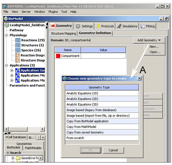
VCell Geometry Editor (VCell Beta 5.0) includes tools for creating geometries both analytically and from experimental images.

Figure 5.

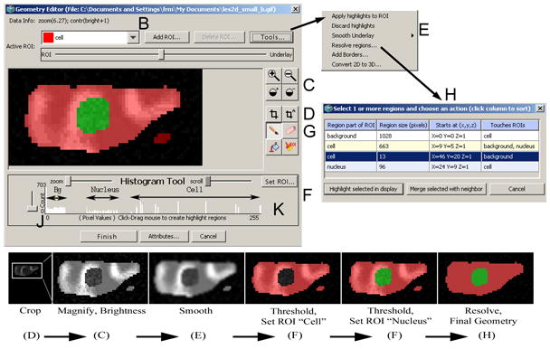
Segmentation of an imported image. The Image Geometry Editor window includes tools for adjusting an uploaded image (cropping (D), magnifying, and adjusting of brightness (C)), as well as tools for segmenting the image ((E), (F), (J), (K), and (H)) necessary for creating a valid VCell geometry.

The overall segmentation process generally begins by clicking the “Add ROI…” button (see (B) in Fig. 5) to add an ROI name for each subdomain (compartment) in the final geometry. The user enters an ROI name and a color is assigned that will be used to paint changes onto the editing canvas when user actions occur. When working with an imported image, the user can crop it to select the appropriate working area (D) and adjust brightness and magnification (C) to clearly display the image before defining ROIs. This is illustrated by the first two frames in the series of snapshots at the bottom of Fig. 5 that demonstrates, stage by stage, how an uploaded noisy image is transformed into a model geometry. In the example of Fig. 5, two spatial compartments are represented by the two corresponding ROIs.

Images that are not pre-segmented often require “smoothing” (blurring) in order to reduce random intensity variations (noise), which otherwise might make thresholding of image intensities less effective. The smoothing function, located under the “Tools…” popup menu, applies a filter to the imported image that reduces random noise (E). If after smoothing the image retains sufficient clarity and definition, the histogram thresholding tool can be applied to select intensity values that will define the currently active ROI (F). This tool allows the user to quickly paint the editing canvas at appropriate locations in all z-slices. Manual painting can be used to add, clean up or enhance ROIs after applying the histogram tool on an imported image or when the user is creating irregular geometry without an imported image (G). The final step in the segmentation process is to apply the “Resolve regions…” tool under the “Tools…” popup menu. This tool calculates the identity, size and location of all contiguous ROIs that have so far been defined in the editing canvas and provides a clear view of the current editing state (H). Without the resolve regions view, it would be difficult to detect small discrepancies in ROI editing, which may lead to a fragmented or inappropriate final geometry unintended by the user. The histogram threshold tool (F), manual paint (G) and resolve regions (H) can be repeated as necessary to create all the ROIs that are appropriate for the desired geometry. Clicking the “Finish” button completes the process of transforming the editing canvas into a valid VCell geometry while allowing the user a chance to continue editing if any errors are encountered. Below, the tools for histogram thresholding and resolving regions are described in more details.

The histogram thresholding tool (F) helps segment an imported image by grouping areas of an image on the basis of their pixel values (a histogram of image intensities will appear below the image geometry editing canvas (J)). This tool is especially helpful when the imported image files have multiple image z-slices representing three-dimensional (3D) information. Manual segmentation of 3D images is tedious and difficult, given that only one z-slice can be viewed at a time. Thresholding of image values is usually effective because structurally related areas of the imported image have close pixel values since they are created similarly during the image generation process (e.g. microscope images from cells stained to enhance cytoplasm or nucleus). Clicking or dragging the mouse horizontally across the histogram display selects a range of pixel values throughout an imported image, that, grouped together, define a portion corresponding to the currently active ROI. Histogram selections are highlighted in the editing canvas and can be applied permanently (painted) by pressing the “Set ROI…” button (K).

The “Resolve regions” tool is activated by clicking “Resolve regions…” in the “Tools…” popup menu and displays a list of all contiguous ROI regions (objects) and their immediate neighbors which are currently “painted” in the editing canvas. Thresholding and manual editing often leave ROI objects in the editing canvas that are inappropriate. The resolved regions list allows the user to select one or more ROI objects and merge them with a neighbor. A neighbor is an ROI object immediately adjacent to (touching) another ROI object in the editing canvas. Thus, merging allows the user to effectively paint several discrete areas of the editing canvas at once, by selecting from a list and pressing “Merge selected with neighbor”. It replaces (overwrites) the selected ROI object paint value with its neighbor ROI paint value. Depending on the selections made in the resolve regions list, merging can add or remove ROI paint throughout the editing canvas in one easy operation.

More details about creating geometries can be found in the VCell 5.0 User Guide (http://vcell.org).

3.2 Incorporating experimental data in simulations

To run a simulation in VCell, the user must specify initial conditions, e.g. initial concentrations. For spatially resolved models, such conditions represent initial spatial distributions of molecular species of interest. In VCell, the initial conditions for spatial simulations can be either defined analytically by a function of spatial coordinates or based on experimental results such as fluorescence imaging data. The latter is done with the aid of a tool called Field Data Manager. This tool allows a user to initiate simulations using irregular spatial distributions of molecular species observed in the image data. The tool can also be applied to cases where the output of one spatial simulation (e.g. a simulation to determine steady-state distributions of molecular species) serves as initial condition for another simulation (e.g. after a specific stimulus event).

From the algorithmic standpoint, the Field Data Manager generates, and operates on, Field Data Objects. The latter are multiple spatially resolved datasets of one, two or three dimensions. These datasets are organized as rectangular grids containing numerical values. Field Data Objects can contain more than one variable (set of data values) and be defined over multiple time points. Once a Field Data Object has been created (e.g. imported from microscopy image file) it can be used as a function within a VCell application. The Field Data Function behaves as any other mathematical function (e.g. square root, sine, etc…) when being evaluated within a VCell simulation. Field Data Functions essentially act as a lookup table mapping values from an (x, y, z) rectangular data grid in the Field Data Object to an (x, y, z) location in the mesh of a spatial simulation.

Below we give a brief description of the elements of the Field Data user interface that might be useful for a potential user (more information can be found in the VCell 5.0 User Guide, http://vcell.org).

The Field Data Manager display (Fig. 6) provides an overview of current Field Data Objects owned by a VCell user and includes tools for creating, accessing and using the Field Data Objects. The overview section (bottom part) of the Manager display contains a tree-like view of all the Field Data objects the user has created, arranged alphabetically by name. Additional information includes the following items: “Size”, showing the number of elements in the Field Data Object for each spatial dimension (x, y, z); “Origin”, showing the position (x, y, z) of the upper, left, bottom corner in simulation domain space (by default this is assigned (0,0,0) unless reassigned by the user during Field Data creation); “Extent”, showing the size (x, y, z) in the simulation domain space occupied by the Field Data Object data grid; “Times”, showing the time domain associated with each separate data grid defined in the Field Data Object; and “Variables”, showing individually defined data sets within the Field Data Object (all sharing the same Size, Origin, Extent and Time information). Double-clicking the “Variables” item will display an expanded list of the names and type (volume, membrane) of the variables contained within the parent Field Data Object.

Figure 6.

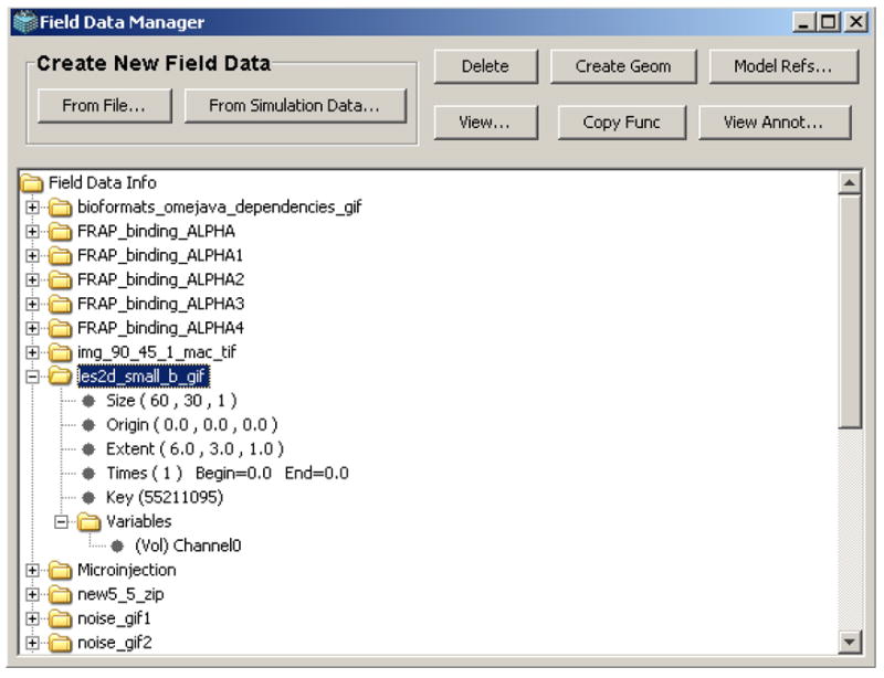
Field Data Manager display. The Field Data Manager tool allows a user to use irregular spatial distributions from experimental images (or simulation results) as initial conditions in VCell models.

The tools in the control section (top part) of the Manager display allow the user to create, manipulate and use Field Data Objects. Field Data Objects can be created in one of two ways. The Objects to be defined by data originated outside the VCell environment (such as microscope image data or numerical data generated with a different program such as MATLAB, MathCAD, etc…) are created using the “From File …” button in the “Create New Field Data” section of the Manager. Provided the dataset can be read by VCell, it will be imported as a Field Data Object. The user will be asked to specify (edit) the Object attributes (a unique Object name not used for any other Object in the Field Data Manager, names of included variables, Origin, Extent, Times) using a “FieldData Info” dialog.

Field Data Objects can also be created from simulations results by using the “From simulation Data…” button. For this, the user must open in advance a corresponding VCell model, containing completed simulation data. A dialog with a table of VCell simulation data that can be used to create a Field Data Object will appear. Selecting a row from the table and pressing the “OK” button will display the “FieldData Info” dialog (see above). The Origin and Extent (“Size (microns)”) and Times information is predefined by the simulation data information and cannot be edited.

To incorporate a Field Data Object into a VCell simulation, a function with a specific syntax is generated. In the BioModel workspace, this function is entered in the “Initial Conditions” section of a spatial application. In the MathModel workspace, this function is simply pasted to the list of functions in the VCML Editor window. The appropriate function syntax is automatically created, once the user selects a variable name from the “Variables” item of a Field Data name in the Field Data Manager display list and presses the “Copy Func” button. If the Field Data Object has multiple time information, a further dialog will appear asking for a particular time which the function ought to reference. The Field Data Function text is copied to the system clipboard and can be pasted into an appropriate application in the BioModel workspace or in the VCML Editor in the MathModel workspace, as described above. For example, if a previously defined Field Data Object had been created and given the Field Data name ‘fdata_gif’ and contained a volume variable named “Channel0” with multiple x, y, z data grids defined for times 0.0 to 5.0 at intervals of .5 seconds, a VCell function created from the spatial data at time 3.5would be defined as “vcField(‘ fdata_gif’,‘Channel0’,3.5,‘Volume’)”. The word “vcField (…)” in the function text is the built-in VCell function name for Field Data and the information within the parentheses (Field Data name, variable name, time point, variable type) tells the VCell where on the VCell server the Field Data information is located. When the user runs a simulation of a VCell model that contains a function vcField(…), the Field Data values are used when the function is called. These values are mapped from the original values used to create a Field Data Object. If the Field Data spatial domain is different from the simulation mesh, the interpolated values are computed, but no interpolation is required if the simulation mesh size is the same as the Field Data size.

Field Data Objects can be deleted only if they are not being used as a Field Data function in any VCell model simulation. A list of all VCell models using a particular Field Data Object can be obtained by pressing the “Model Refs…” button. A table showing the VCell model information will appear if the Field Data Object is referenced. The Field Data Object annotation introduced by the user in the process of creating a Field Data Object can be viewed and edited by pressing the “View Annot…” button. The Field Data Object “image” can be viewed by pressing the “View…” button. A Simulation Results Viewer will appear displaying the Field Data Object as VCell data (see the VCell User Guide under Simulation Results Viewer for further information). Field Data variables can be used as a template for creating new spatial geometries by selecting a name under the “Variables” sub-tree of an expanded Field Data name and clicking the “Create Geom” button. The VCell Geometry Editor will appear preloaded with an image representing values from the selected Field Data variable (see the VCell User Guide under Geometry Editor for more information).

4. New stable solver for spatial simulations in VCell

Given the nature of biological applications, numerical solvers implemented in modeling packages are required to be fast, numerically stable, and accurate. Moreover, they should be highly automated. Software packages developed for simulating biochemical networks (21), including VCell, have long provided robust solvers for systems described by ordinary differential equations (ODEs). In particular, systems biologists have come to rely on so-called stiff solvers that retain their numerical stability and good performance in the presence of vastly disparate time scales – a common situation in biological applications. However, for the case of spatially resolved systems described by partial differential equations (PDEs), solvers that meet such requirements and apply to a general class of problems are less common.

Up until recently, the default VCell spatial solver - based on a fixed step semi-implicit method (5, 12) - required the user to specify the integration time step. Generally, choosing an appropriate time step is a nontrivial task. When the problem is stiff (i.e. includes processes with very different time scales), a small integration time step is necessary for such a solver to be stable, at the expense of significant decrease in solver speed. In biological applications, the stability constraints are often caused by fast reaction kinetics. For cases where a model includes a subsystem of reactions that remain fast throughout the simulated time, VCell has provided an optional quasi-steady state approximation (QSSA) (22), which is automatically invoked if the user labels certain reactions as “fast”. In VCell, implementation of QSSA for spatial models is similar to operator-splitting techniques (23) in that the system is updated due to slow and fast processes in separate sub-steps, with instantaneous equilibration of fast reactions at the second sub-step. This technique is efficient and accurate when the difference in the time scales is large, but it does not apply to situations in which reactions become fast later in the simulation, or for cases of moderately stiff reactions for which a steady state approximation is not adequate, but that are fast enough to produce unstable answers if one is not careful in choosing the time step.

Below we describe a new stiff spatial solver that has been recently implemented in VCell and deployed for general use. The solver meets requirements of numerical stability and efficiency that modelers are used to in non-spatial simulators of biochemical networks. With a built-in automatic time-step control, the new VCell spatial integrator is essentially turn-key. In combination with automatic meshing, the solver can also be used as a module in standalone applications designed for specific purposes, such as Virtual FRAP (24). It is freely accessible through the VCell user interface (www.vcell.org).

The design of the new stiff spatial solver in VCell is based on the well-known method of lines (MOL) (25): after applying spatial discretization, a system of PDEs is replaced with a large system of ODEs, which is then solved using a stiff ODE solver. The stiff solver advances the solution in time using implicit differentiation formulas and adaptive time step control. At each step in time, a large coupled nonlinear system of algebraic equations must be solved. A commonly used alternative called operator-splitting (26) avoids solving large, coupled nonlinear systems, but it can carry more error and is not always applicable, especially in situations when stiffness originates from binding of molecules to membranes, interactions that are represented in terms of fast, nonlinear boundary conditions. The fully implicit approach, although sometimes dismissed as inefficient because of the large size and complexity of the non-linear solves, can in fact be efficient when implemented with the use of effective technologies designed to optimize storage requirements and computation time. In particular, the adaptive control of the time step and order of the integration method, the use of Jacobian-free Newton-Krylov methods (see e.g. (27) and references within) for solving large-scale sparse nonlinear systems, and the application of effective physics-based preconditioners are the main ingredients that contribute to the robustness and good performance of this solver.

In our implementation, we employ a conservative finite volume spatial discretization scheme with special treatment at and near membranes (14). The resulting system of ODEs is solved using CVODE, a solver from the SUNDIALS library (28), designed for stiff and non-stiff initial value problems. CVODE implements multistep methods of variable order of accuracy and automatic control of the integration time step, so that both the method and the integration time step are adjusted adaptively based on local error estimates and prescribed tolerances. Typically, the method of lines generates nonlinear algebraic systems that are large but have a sparse Jacobian (this is due to the local nature of grid connectivity in the spatial discretization). The solvers in SUNDIALS deal efficiently with this situations. Their Jacobian-free Newton-Krylov methods allow for customized preconditioners for the linear iterative solver module. (A preconditioner is a linear operator designed to accelerate the convergence of an iterative method (29). Solving a system Ax=b with preconditioning could be seen as solving an equivalent system, for example P^-1 Ax=P^-1 b (although the matrix multiplication operation is not actually carried out). If the preconditioner P^-1 approximates the inverse of A in some way, the new system can be solved in fewer iterations than the original system. For a precondtioner to be effective, a system of the form Py=r should be easy to solve.) In the current VCell implementation, we generate a preconditioner based on (modified) incomplete LU factorization of the diffusion operator inside each compartment. Because it is sparse and block-diagonal (thus simplifying the coupling between variables and spatial coupling between compartments, yet capturing some of the local coupling), the preconditioner provides an economical way to accelerate the convergence of the linear solver provided in SUNDIALS for the Jacobian system in Newton’s method.

The new VCell spatial solver was tested and deployed for general use. Test results indicate the practically unconditional stability of the solver. The solver’s efficiency is greatly enhanced by the adaptive time-stepping in CVODE: the required accuracy is maintained by applying small time steps during periods of rapid change in the solution, whereas the time step is allowed to safely grow outside of these periods. The ability to use larger steps in a stable way is one important reason for the solver’s good performance. Just as important is using the Jacobian-free Newton-Krylov methods, combined with our custom-designed preconditioner for solving the linearized system. Our tests indicate that not only does the new spatial solver outperform our original semi-implicit PDE solver in stiff applications, but it is also sufficiently fast when applied to moderately stiff or non-stiff problems.

As an example, we present the results obtained for a test case of a moderately stiff 2D reaction-diffusion system in which stiffness arises from fast membrane fluxes. The test case involves a simple model of a ‘local excitation-global inhibition (LEGI)’ mechanism employed in theories of chemotaxis (30, 31). In the model, spatial gradients of active and inactive forms of a protein P inside the cell Ω arise from a combination of activation by the membrane-associated enzyme E, uniformly distributed along a front fragment ∂Ω_E of the cell membrane ∂Ω, and linear inhibition occurring throughout the cell. The enzymatic activation follows a classical two-step kinetic scheme, P + E ↔ EP → P_a + E (32): fast reversible binding between inactive P and E results in an intermediate complex EP and is followed by a relatively slow irreversible release of the activated protein P_a. Note that this simple test model does not include upstream events in which the enzyme gets activated by a chemoattractant; rather, the spontaneous inactivation of the enzyme is simply balanced by a continuous activation. In the tests, we used an irregular 2D geometry (Fig. 7), reminiscent of shapes of polarized motile cells. For this system, which involved two volume variables and two membrane variables and was solved on a grid with 13000 mesh points, the original non-stiff VCell solver took 10⁵ time steps. By comparison, the new stiff solver without a preconditioner solved the same problem using a total of 8980 time steps of variable size, and when the preconditioner was supplied, only a total of 887 steps were needed. The computing times for these three runs were, respectively, 24 min, 11 min and 1.1 min. An increase in stiffness in this model did not significantly affect performance of the stiff solver, while the semi-implicit solver became dramatically slower.

Figure 7.

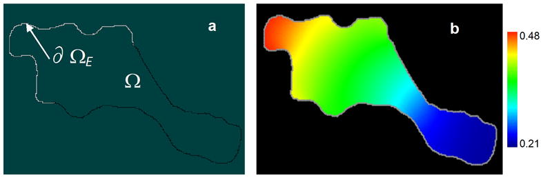
A simple version of the local excitation - global inhibition (LEGI) model (30, 31): (a) simulation geometry and (b) steady-state concentration gradients of the active form of a protein, P_a, in arbitrary units.

There is room for further improvements. The preconditioner described above does not incorporate information about reaction rates or membrane fluxes - only the diffusion terms. In cases when other terms become a dominant part of the operator, the above preconditioner becomes less effective, forcing the linear solver within Newton’s method to perform more iterations, and sometimes forcing the CVODE solver to reduce the time step. A more sophisticated preconditioner is being developed that takes reaction terms into account and can be more effective in certain cases.

References

- 1.Loew LM, Schaff JC. The Virtual Cell: a software environment for computational cell biology. Trends Biotechnol. 2001;19:401–6. doi: 10.1016/S0167-7799(01)01740-1. [DOI] [PubMed] [Google Scholar]
- 2.Moraru II, Schaff JC, Slepchenko BM, Loew LM. The virtual cell: an integrated modeling environment for experimental and computational cell biology. Ann N Y Acad Sci. 2002;971:595–6. doi: 10.1111/j.1749-6632.2002.tb04535.x. [DOI] [PubMed] [Google Scholar]
- 3.Moraru II, Schaff JC, Slepchenko BM, Blinov ML, Morgan F, Lakshminarayana A, et al. Virtual Cell modelling and simulation software environment. IET Syst Biol. 2008;2:352–62. doi: 10.1049/iet-syb:20080102. [DOI] [PMC free article] [PubMed] [Google Scholar]
- 4.Slepchenko BM, Schaff JC, Carson JH, Loew LM. Computational cell biology: spatiotemporal simulation of cellular events. Annu Rev Biophys Biomol Struct. 2002;31:423–41. doi: 10.1146/annurev.biophys.31.101101.140930. [DOI] [PubMed] [Google Scholar]
- 5.Slepchenko BM, Loew LM. Use of Virtual Cell in studies of cellular dynamics. Int Rev Cell Mol Biol. 2010;283:1–56. doi: 10.1016/S1937-6448(10)83001-1. [DOI] [PMC free article] [PubMed] [Google Scholar]
- 6.Schaff J, Loew LM. The virtual cell. Pac Symp Biocomput. 1999:228–39. doi: 10.1142/9789814447300_0023. [DOI] [PubMed] [Google Scholar]
- 7.Schaff J, Fink CC, Slepchenko B, Carson JH, Loew LM. A general computational framework for modeling cellular structure and function. Biophys J. 1997;73:1135–46. doi: 10.1016/S0006-3495(97)78146-3. [DOI] [PMC free article] [PubMed] [Google Scholar]
- 8.Schaff JC, Slepchenko BM, Loew LM. Physiological modeling with virtual cell framework. Methods Enzymol. 2000;321:1–23. doi: 10.1016/s0076-6879(00)21184-1. [DOI] [PubMed] [Google Scholar]
- 9.Loew LM, Schaff JC, Slepchenko BM, Moraru II. The Virtual Cell Project. In: Liu E, Lauffenburger DA, editors. Systems Medicine: Concepts and Perspectives. San Diego: Academic Press, Elsevier Inc.; 2010. pp. 273–288. [Google Scholar]
- 10.Andrews SS, Addy NJ, Brent R, Arkin AP. Detailed simulations of cell biology with Smoldyn 2.1. PLoS Comput Biol. 2010;6:e1000705. doi: 10.1371/journal.pcbi.1000705. [DOI] [PMC free article] [PubMed] [Google Scholar]
- 11.Andrews SS, Bray D. Stochastic simulation of chemical reactions with spatial resolution and single molecule detail. Phys Biol. 2004;1:137–151. doi: 10.1088/1478-3967/1/3/001. [DOI] [PubMed] [Google Scholar]
- 12.Slepchenko BM, Schaff JC, Macara I, Loew LM. Quantitative cell biology with the Virtual Cell. Trends Cell Biol. 2003;13:570–6. doi: 10.1016/j.tcb.2003.09.002. [DOI] [PubMed] [Google Scholar]
- 13.Schaff JC, Slepchenko BM, Choi YS, Wagner J, Resasco D, Loew LM. Analysis of nonlinear dynamics on arbitrary geometries with the Virtual Cell. Chaos. 2001;11:115–131. doi: 10.1063/1.1350404. [DOI] [PubMed] [Google Scholar]
- 14.Novak IL, Gao F, Choi Y-S, Resasco D, Schaff JC, Slepchenko BM. Diffusion on a Curved Surface Coupled to Diffusion in the Volume: Application to Cell Biology. J Comput Phys. 2007;226:1271–1290. doi: 10.1016/j.jcp.2007.05.025. [DOI] [PMC free article] [PubMed] [Google Scholar]
- 15.Rosenberg S. The Laplacian on a Riemannian Manifold. Cambridge: University Press; 1997. [Google Scholar]
- 16.Sbalzarini IF, Hayer A, Helenius A, Koumoutsakos P. Simulations of (an)isotropic diffusion on curved biological surface. Biophys J. 2006;90:878–885. doi: 10.1529/biophysj.105.073809. [DOI] [PMC free article] [PubMed] [Google Scholar]
- 17.Schwartz P, Adalsteinsson D, Colella P, Arkin AP, Onsum M. Numerical computation of diffusion on a surface. Proc Natl Acad Sci U S A. 2005;102:11151–6. doi: 10.1073/pnas.0504953102. [DOI] [PMC free article] [PubMed] [Google Scholar]
- 18.Leibon G, Letscher D. Delaunay triangulations and Voronoi diagrams for Riemannian manifolds. Proceedings of 16th Annual Symposium on Computational Geometry; Hong Kong. 2000. pp. 341–349. [Google Scholar]
- 19.Ferziger JH, Peric M. Computational Methods for Fluid Dynamics. 3. Springer; 2002. [Google Scholar]
- 20.Moissoglu K, Slepchenko BM, Meller N, Horwitz AF, Schwartz MA. In vivo dynamics of Rac-membrane interactions. Mol Biol Cell. 2006;17:2770–9. doi: 10.1091/mbc.E06-01-0005. [DOI] [PMC free article] [PubMed] [Google Scholar]
- 21.Alves R, Antunes F, Salvador A. Tools for kinetic modeling of biochemical networks. Nat Biotechnol. 2006;24:667–72. doi: 10.1038/nbt0606-667. [DOI] [PubMed] [Google Scholar]
- 22.Slepchenko BM, Schaff JC, Choi YS. Numerical Approach to Fast Reactions in Reaction-Diffusion Systems: Application to Buffered Calcium Waves in Bistable Models. J Comput Phys. 2000;162:186–218. [Google Scholar]
- 23.Yanenko NN. The Method of Fractional Steps. New York: Springer; 1971. [Google Scholar]
- 24.Cowan AE, Li Y, Morgan FR, Koppel DE, Slepchenko BM, Loew LM, et al. Using the Virtual Cell Simulation Environment for Extracting Quantitative Parameters from Live Cell Fluorescence Imaging Data. Microscopy Today. 2009;17:36–39. [Google Scholar]
- 25.Schiesser WE. The Numerical Method of Lines: Integration of Partial Differential Equations. San Diego: Academic Press; 1991. [Google Scholar]
- 26.Sportisse B. An analysis of operating splitting techniques in the stiff case. J Comput Phys. 2000;161:140–168. [Google Scholar]
- 27.Knoll DA, Keyes DE. Jacobian-free Newton-Krylov methods: a survey of approaches and applications. J Comput Phys. 2004;193:357–397. [Google Scholar]
- 28.Hindmarsh AC, Brown PN, Grant KE, Lee SL, Serban R, Shumaker DE, et al. SUNDIALS: Suite of Nonlinear and Differential/Algebraic Equation Solvers. ACM Transactions on Mathematical Software. 2005;31:363–396. [Google Scholar]
- 29.Saad Y. Iterative Methods for Sparse Linear Systems. 2. Philadelphia, PA: SIAM; 2003. [Google Scholar]
- 30.Levchenko A, Iglesias PA. Models of eukaryotic gradient sensing: application to chemotaxis of amoebae and neutrophils. Biophys J. 2002;82:50–63. doi: 10.1016/S0006-3495(02)75373-3. [DOI] [PMC free article] [PubMed] [Google Scholar]
- 31.Yang L, Iglesias PA. Modeling spatial and temporal dynamics of chemotactic networks. Methods Mol Biol. 2009;571:489–505. doi: 10.1007/978-1-60761-198-1_32. [DOI] [PMC free article] [PubMed] [Google Scholar]
- 32.Keener J, Sneyd J. Mathematical Physiology. New York: Springer; 1998. [Google Scholar]