

Abstract
Soft x-ray tomography (SXT) is a powerful imaging technique that generates quantitative, 3D images of the structural organization of whole cells in a near-native state. SXT is also a high-throughput imaging technique. At the National Center for X-ray Tomography (NCXT), specimen preparation and image collection for tomographic reconstruction of a whole cell require only minutes. Aligning and reconstructing the data, however, take significantly longer. Here we describe a new component of the high throughput computational pipeline used for processing data at the NCXT. We have developed a new method for automatic alignment of projection images that does not require fiducial markers or manual interaction with the software. This method has been optimized for SXT data sets, which routinely involve full rotation of the specimen. This software gives users of the NCXT SXT instrument a new capability - virtually real-time initial 3D results during an imaging experiment, which can later be further refined. The new code, Automatic Reconstruction 3D (AREC3D), is also fast, reliable and robust. The fundamental architecture of the code is also adaptable to high performance GPU processing, which enables significant improvements in speed and fidelity.
Keywords: 3D imaging, image processing
Introduction
Soft X-ray tomography (SXT) is the only imaging technique that generates high-resolution, 3D views of cellular structures in large (up to 15 microns diameter), intact eukaryotic cells in the near-native state. Because SXT is conducted in the ‘water window’, the region of the spectrum where carbon and nitrogen absorb an order of magnitude more than water, it is particularly sensitive to the distribution of organic molecules in a cell. Absorption of photons at this wavelength adheres to Beer-Lambert’s law and is therefore linear with thickness (Attwood, 1999). Consequently SXT images are uniquely quantitative, and each organelle is seen based on its organic composition, which gives it a unique linear absorption coefficient (LAC) measurement (Le Gros et al., 2005; Weiss et al., 2000). The difference in the LAC values of cellular components yields high-contrast images without the need for any chemical stains.
Cells imaged with SXT are typically between 1–15 microns in diameter, and each image shows all internal organelles superimposed in a 2D projection image. Tomographic reconstruction methods make it possible to retrieve that information and generate 3D views that reveal the spatial distribution of the organelles. It is well known that the optimal 3D reconstruction is achieved when images are taken at multiple intervals through 180 degrees. With electron tomography, the combination of thin, planar specimens and the mechanical constraints of the specimen holders for these samples limits the ability to acquire images at all angles, and the quality of the reconstruction is compromised. Algorithms have been devised to minimize the artifacts in the reconstruction, but it is still not possible to obtain isotropic resolution. SXT can circumvent this problem by imaging cells in thin-walled (200 nm thin) capillary tubes. Images of cells in a capillary can be collected through an angular range of 180, or even 360 degrees to more evenly distribute the x-ray dose. As a consequence there is no wedge of missing information and, due to the incoherent bright field imaging geometry (Streibl, 1985), fully isotropic resolution can be achieved in the reconstructions. Full-rotation imaging has been used very successfully with SXT to generate 3D images of a wide variety of cell types with isotropic resolution (Carrascosa et al., 2009; Le Gros et al., 2005; McDermott et al., 2009; Meyer-Ilse et al., 2001; Schneider et al., 2010; Uchida et al., 2009; Uchida et al., 2011).
The first step in processing data for high-resolution tomography involves the alignment of the projection images taken at different angles to a common axis of rotation. This is especially important for high-resolution techniques like electron tomography and SXT where the precision of the rotation axis and overall accuracy and stability of the specimen stage are at, or just below, that required by the limiting resolution of the imaging technique. Currently, the “gold standard” that gives the best possible alignment of soft x-ray tomography data is alignment based on fiducial markers. Experimentally, gold nanoparticles are added directly to the sample, or to the sample container. Each nanoparticle is a fiducial marker that can be tracked through the series of projection images. By tracking multiple markers, all of the images can be aligned to a common frame of reference with an error of one pixel or less (Kremer et al., 1996). Alignment of fiducial markers can be done manually, but this is a very time consuming and labor intensive process. Since SXT can image large numbers of cells in a relatively short period of time (Uchida et al., 2009), there is an obvious need to automate the alignment process.
There are many approaches to automating the tracking of fiducial markers through a stack of projection images, including IMOD (Kremer et al., 1996) XMIPP (Sorzano et al., 2004) and others (Amat et al., 2008; Chen et al., 1996; Liu et al., 1995; Zheng et al., 2007); for review, see Brandt (Brandt, 2006) and (Frank, 2006; Houben and Bar Sadan, 2011). Most of these programs have been developed to process data for electron tomography, which examines specimens that must be less than 1 micron along the optical axis of the microscope. These automated programs have not been as successful aligning images for x-ray tomography, which examines large cylindrical specimens (frequently up to 15 microns thick) filled with numerous high contrast structures. With SXT there is significantly less difference between the contrast levels of the gold markers and cellular structures, which makes it difficult to follow the markers through the full rotation.
The simplest automated alignment approach is the cross-correlation approach, in which appropriate transforms between images are calculated pairwise for images in the projection stack (Kremer et al., 1996). A second approach is feature-based alignment. In this method, rather than relying on gold nanoparticles as fiducial markers, feature points (such as Harris corners (Harris and Stephens, 1988)) are extracted from the images themselves, and these are used as the fiducial markers that are tracked across the image stack (Castano-Diez et al., 2010; Castano-Diez et al., 2008b; Sorzano et al., 2009; Winkler and Taylor, 2006). A third approach is known as a 3D model-based method, in which an initial alignment is used to generate a tomographic reconstruction, and the projections are iteratively aligned to this volume and then used to generate a new refined volume (Amat et al., 2010). An excellent example of this approach is described in (Yang et al., 2005). This approach can yield excellent results, though it is computationally intensive, and the initial coarse alignment must be relatively good in order to yield the global minimum. After exploring these three approaches to SXT data alignment, we found that model-based alignment produced the best results with SXT data. Much of the model-based software that has been developed for electron tomography, however, is targeted at single-particle cryoelectron microcroscopy, which involves a large number of projections (often many 1000s), each of which is relatively small (below 100^2 pixels); thus, the available software has imposed limits on the size of images in terms of required computer memory. With SXT, we use fewer projection images (between 90 and 360), with each image being much larger (either 1024^2 or 2048^2). To obtain an optimal solution for aligning SXT data, we developed model-based alignment software uniquely suited for x-ray images. The resulting software package, Automatic Reconstruction 3D (AREC3D), is central to the data processing pipeline used at the NCXT. The source code for AREC3D is available at https://codeforge.lbl.gov/projects/arec3d. In this manuscript we describe the AREC3D methodology and present examples of aligned SXT data sets.
Results
Data processing programs operate on the assumption that the axis of rotation lies vertically. Since the long, thin custom-made glass capillary specimen holders used for SXT are not perfectly cylindrical, this is not always the case. Consequently there can be a small angle between the real axis of rotation (y) and the vertical axis of the CCD chip (Y), as diagrammed in Figure 1. Additional imperfections in the rotation and translation stages cause additional movements of the specimen, which are not in accord with the model implicit in a standard tomographic reconstruction procedure. Figure 2 shows the first and last images from an unaligned series of projection images collected through 180 degrees. Strictly speaking the alignment correction can only be computed in a complete 3-dimensional space. However, given the geometry of our specimen holders, angular changes are relatively small, and good alignment and reconstruction results can be achieved by limiting alignment parameters to translations and one rotation in the plane of the projection images. With this approach we are taking into account differences between the angle of rotation and the vertical direction in the plane of imaging; components outside of this plane are ignored. As a result an independent tomographic reconstruction can be implemented in slices along the rotation axis (Castano-Diez et al., 2006; Fernandez, 2008; Mastronarde, 2008). Figure 3 shows a comparison of digital orthoslices through a tomographic reconstruction of a yeast cell where the projections were aligned by translation cross-correlation and manual fiducial alignment. It is clear that the cross-correlation alignment is not sufficient in this case to give useful results. The main issue with this method by itself is that it is not robust and it produces inconsistent results frequently failing to produce a useable reconstructed SXT data set.
Figure 1.
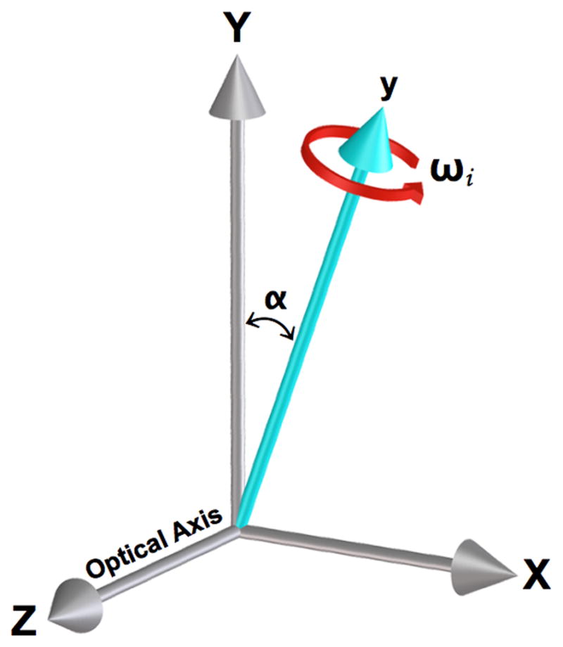
Simplified diagram illustrating an example of a rotational error that occurs during collection of images for a tomographic data set. The experimental rotational axis (y) is offset from the assumed reconstruction axis (Y) by angle α, ωi is the angle of the ith projection image. The X and Y axes are parallel to the CCD pixel rows and columns, respectively. Additional misalignments can occur due to other rotation and translation stage errors.
Figure 2.
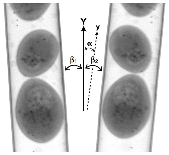
Projection images of a capillary filled with S. cerevisiae yeast cells. The images were taken at 0 and 180 degrees. The angular deviation of the experimental rotation axis (y) can be estimated by measuring the angle between the tube edges and Y axis, with β1 the angle for the 0-degree projection and β2 the 180-degree projection. The tube wall is coated with gold markers used as fiducial markers for manual alignment. Scale bar = 1 um.
Figure 3.
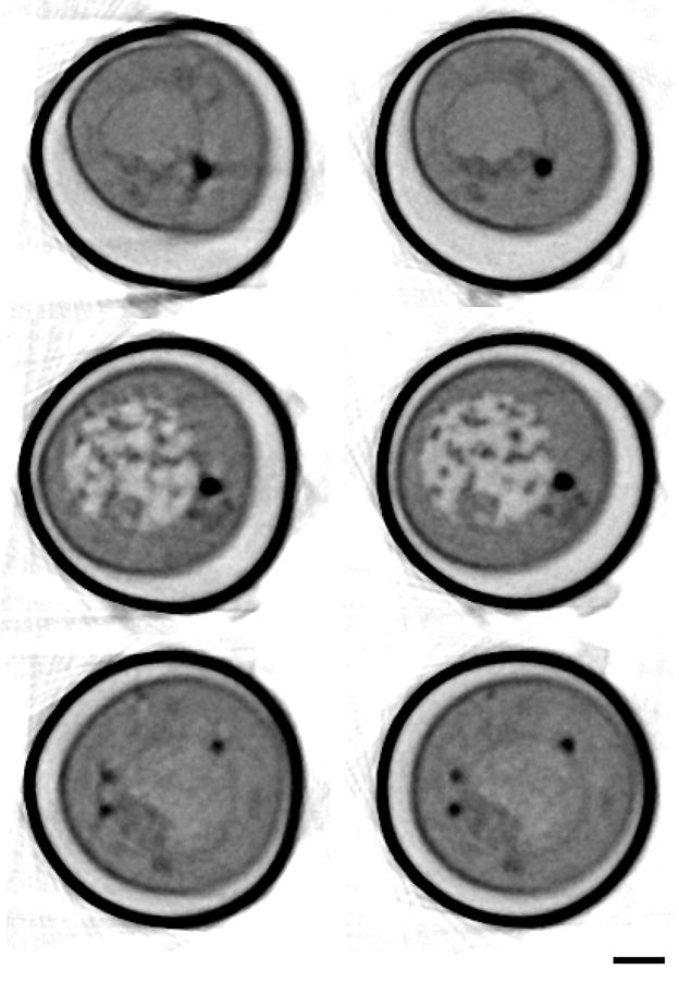
Digital orthoslices through tomographic reconstructions of a yeast cell where projections were aligned by cross-correlation (left) and manual fiducial alignment (right). Orthoslices shown were from different positions along the tube axis. Distortions are clearly visible in the images aligned by cross-correlation shown on the left. Scale bar 1 micrometer. Ice crystals seen on the surface of the tube are from contamination during specimen transfer to the x-ray microscope; they do not interfere with imaging due to the highly penetrating nature of x-rays at the imaging energy.
Alignment Strategy
To discuss our alignment strategy, we first look at the geometric relationship between the 3D object to be reconstructed and its 2D projection images. During the image acquisition process, the sample is placed in a roughly cylindrical capillary tube that is rotated around an axis (y) through an angle, ωi. The axis of rotation may not be in the center of the cylindrical tube. Furthermore, the axis of rotation may not be parallel to the Y-axis (the vertical axis of the CCD camera, which is the vertical axis of the projection images), and the angle between the true axis of rotation (y) and the Y-axis may change as the tube is rotated due to stage imperfections. In addition to a tilt of the axis, stage drift may also produce horizontal and vertical shifts. The lack of a priori knowledge about the location of the rotation axis and the additional orientation changes due to the vibration of the stage makes the alignment and reconstruction problem a nontrivial task. The alignment strategy we developed aims to detect the inconsistency among different projection images and correct for the misalignment introduced by the systematic experimental errors.
If we assume the noise in the image is moderate, and can be described by a Gaussian distribution with zero mean, the alignment and reconstruction problem can be formulated as a nonlinear least squares problem of the form
| (1) |
where f is the 3D object to be reconstructed, (ψj, φj) are two of the Euler angles that describe the orientation of the 3D object that yields the jth projection image bj. The projection image can be viewed simply as the a 2D image formed by applying a line integral operator P to the 3D object along a prescribed direction after the 3D object has been rotated by (ψj, φj), and translated by sj (Yang et al., 2005). The azimuthal rotation angles are assumed to be known exactly, and for the single tilt-axis geometry the remaining Euler angles represent an in-plane rotation.
The optimization problem defined in (1) is generally difficult to solve due to the nonlinear coupling between the unknown 3D object and the orientation parameters ψj and φj. One way to solve the problem, which is widely used in the cryoEM community, is to perform what is called a projection matching (Penczek et al., 1994). The projection matching algorithm can be viewed as a generalized coordinate descent algorithm. It requires an initial guess of the 3D object f (or the Euler angles ψj and φj) f0 and consists of the following two steps:
When f0 is available, an exhaustive search of the optimal orientation parameters ψj and φj is performed, i.e, we first solve
Once an optimal set of ψj and φj are determined, we can solve a linear least square problem by using a standard tomographic reconstruction algorithm, i.e., we solve
One of the key factors that affect the convergence of the projection matching algorithm is the availability of a good initial guess f0. For cryoEM image reconstruction, obtaining a good initial guess is generally a difficult task because the geometric relationship between the 3D object and 2D projection images is largely unknown a priori. However, for X-ray cell imaging, we have a better knowledge of the relationship between the projection image and the object even though we do not have the precise values of some of the orientation and translational parameters. In particular, the azimuthal rotation angles are known exactly, and in practice we have at least 91 images cover 180 degree viewing angles in 2-degree increments. In addition, the presence of the capillary tube edges in the projection images enables us to perform an initial alignment to fix the axis of rotation and obtain an initial estimate of the direction of the rotation axis relative to the y-axis.
To identify the angle between the actual rotation axis and the Y-axis, we first identify the tube edges associated with the 1st and the 91st images by using standard edge detection techniques. Without loss of generality, we can assume the azimuthal rotation angles associated with these two images are 0 degree and 180 degrees. From the slope of these edges, we can calculate the angles between the tube edges and the Y-axis. If we denote the angle between the tube edges of the first image and the Y-axis by β1, and that associated with the 91st image by β2, and if we ignore additional rotation introduced by stage imperfections, then the angle α between the rotation axis and the Y-axis should be α=(β1+ β2)/2 (see Figure 2).
By rotating each image by α degrees, we effectively make the axis of rotation parallel to the y-axis. However, the axis rotation does not necessarily pass the origin of the 3D coordinate space, nor does it have to be in the center of the tube. Although the quality of the 3D reconstruction does not depend on the exact location of the axis of rotation, computational efficiency can be gained if we choose the axis of rotation to go through the center of the tube. In this case, total size of the reconstruction volume is roughly the size of the cylindrical tube with little extra void space outside of the tube.
To correct for translational movement of the rotation axis resulting from the vibration of the stage, we perform a successive translational alignment between the ith and the i+1st images for i = 1,2,…,90 using cross correlation. Such an alignment procedure eliminates most of the translational movement that depends on the azimuthal rotation angle θ. To account for a potentially global (angular independent) horizontal drift of each projection image by an unknown constant number of pixels Δ, we flip the 91st image in the horizontal direction and cross correlate the flipped image with the first image. Because the x-coordinate of each pixel in the 1st and the 91st images can be represented by
and
respectively, where (x0,y0) is the unknown (x,y) location of the rotation axis, the position of cross correlation peak yields 2Δ, which allows us to deduce the constant drift and shift each image by -Δ pixels to correct for such a drift. A similar correction can be made for a vertical drift also.
After the initial alignment steps described above have been performed, we crop each projection image to keep the projection of the sample and the capillary tube in the image. We then choose the axis of rotation to be in center of the cropped image and perform an initial 3D tomographic reconstruction. Because the axis of rotation is fixed, the 3D reconstruction can be reduced to ny 2D reconstructions, were ny is the number of (x,z) slices in the y-direction. A number of algorithms can be used to perform the reconstruction task. We use the conjugate gradient (CG) algorithm because it produces a high quality reconstruction, is efficient and relatively easy to parallelize on a distributed-memory cluster. Typically, 15 or fewer CG iterations are sufficient to produce a 3D reconstruction with desired resolution. Running too many CG iterations may amplify undesirable noise in the data. The iteration number can be viewed as a regularization parameter for the CG based iterative reconstruction algorithm (Hansen, 1998).
The additional azimuthal angular dependent in-plane rotations of the projection images introduced by imperfections in the stage are corrected in a simplified projection matching procedure that follows the initial alignment. In this simplified projection, we generate a set of reference projections from a 3D model constructed in the previous iteration computationally. Both translation and rotational cross-correlations are performed between each reference projection image and the corresponding experimental image (after it is properly cropped). The translational shifts and in-plane rotation angles are used to transform each experimental image before the transformed images are cropped and used to produce a new 3D reconstruction. This procedure is repeated until the changes in shifts and angles fall below a chosen threshold. The flowchart in Figure 4 gives a summary of our alignment procedure.
Figure 4.

An overview of the methodology we use for automatic alignment of projections prior to soft x-ray tomographic reconstruction. First, each image in the projection stack is aligned to the projection images from adjacent angles by cross correlation. This allows the construction of a coarsely aligned projection image stack by applying transforms to the original images. Second, the position of the center of rotation with respect to the images is determined and a global in-plane rotation is determined. Third, an initial tomographic reconstruction is generated. Fourth, at each angle at which a projection image was collected in the original data set, a re-projection is generated from the reconstructed 3D model volume. Fifth, these re-projections are compared with the original projection images, and the transform needed to align each original projection to the re-projection from the model at that angle is refined. Finally, steps three through five are repeated iteratively; with each iteration, the reconstructed volume improves as the alignment errors decrease.
In implementing the code, we focused on MPI (message passing interface) parallelization for distributed memory clusters that have a limited amount of local memory (Pacheco, 2011). Although our parallelization tends to significantly reduce the required time for the reconstruction and alignment process, our main focus in the distributed-memory parallel implementation is to address the memory-limitation problem. The alignment and reconstruction procedure described above requires two different types of data distribution schemes that are currently coordinated through disk I/O. For the initial alignment, it is natural to distribute experimental images among different processing units. Each processing unit contains a fixed number of images. Successive translational alignment is performed simultaneously on local images assigned to individual processors. The aligned images are written to the disk as a single image stack, which requires synchronization. When the image stack containing the aligned images is read into the memory again for reconstruction, each image is partitioned evenly along the y direction, and each processing unit receives m sub-images that it can use to reconstruction a portion of the 3D object.
In the simplified projection matching procedure, reference sub-images are generated from a partial 3D volume produced from the previous iteration, the reference sub-images are merged when they are written to the disk as a single file. The merged reference images are read back from the disk and redistributed among different processors on an image-by-image basis so that the cross-correlation between the reference projection and experimental images can be performed in parallel.
To characterize the performance of AREC3D, we measured wall clock time while running it with different numbers of processors for a data set with 91 projections that was originally 1024 × 1024 pixels, then cropped to 500 × 800 pixels. For 1, 2, 4, 8, 16, 32, 64, and 128 processors, the time to complete one iteration was 1600, 800, 410, 225, 120, 72, 56, and 35. As the number of processors increases, it becomes difficult to divide 91 images evenly among processors. In addition, I/O overhead means that the scaling is not perfectly linear.
Although our current parallelization scheme incurs some I/O overhead, the overhead is moderate. Even though the total amount of memory for the latest machines tends to increase, memory per processing unit remains the same, and is projected to decrease in the future. Therefore, we decided to perform I/O in this version of the code to make it more flexible. We are also developing a shared-memory parallel version of the code that can be used on a multi- and many-core mode with a large amount of shared memory using OpenMP. The OpenMP version does not use any I/O other than reading the 2D images and writing out the reconstructed 3D reconstruction. This version will be modified to run on a GPU using CUDA. In addition, we plan to develop a hybrid MPI and OpenMP parallel version of the code that can be used on multi- and many-core clusters (Agulleiro and Fernandez, 2011; Castano-Diez et al., 2008a; Xu et al., 2010).
Testing and Validation
In this section we present results on the testing and validation of our method using two data sets: an artificially generated phantom, and a representative SXT data set. The test phantom was generated using a combination of Matlab scripts and functions from a freely available image reconstruction toolbox (Fessler, 1995; Fessler, 2009). The 3D phantom is modeled as a water-filled glass tube in which there is an ellipsoidal cell that contains one high-contrast and one low-contrast internal organelle. Nanoparticles attached to the outside wall of the tube were built into the model for use in manual alignment procedures. The soft x-ray absorption characteristics of the objects in the phantom were chosen to match those obtained from SXT measurements of real cells. The axis of the capillary was chosen to lie imprecisely along the y-axis of the volume. Projections were generated from this noiseless phantom at 2 degree increments over 180 degrees. We then added noise to the projections based on actual noise characteristics measured using the NCXT soft x-ray microscope, XM2. In addition, we added random in-plane rotations to the phantom projection data. This set of projections was used as the input for both the automatic alignment software as well as for a manual alignment based on the included fiducial markers.
To test real SXT data, we used a set of projection images with fiducial markers. These data served as the input for both automatic alignment and manual alignment based on fiducial markers. We evaluated the quality of the aligned data using visual inspection of the digital orthoslices through the reconstructed volume. A quantitative comparison was obtained using a Fourier Ring Correlation (FRC) calculation using the “noise-compensated leave one out” (NLOO) method of Cardone, Grunewald, and Steven (Cardone et al., 2005). This method works best for data comprised of a limited number of projection images, and in our experience this measurement has been more robust and informative than other FRC methods.
Figure 5 shows one-pixel-thick orthoslices through the reconstructions of both the phantom and the real SXT data set. We aligned the data using both manually selected fiducial markers and the AREC3D software. For the AREC3D alignment results we used 100 iterations of projection matching. Because of the cylindrical geometry of our specimens we have an excellent way to visually measure the quality of an aligned data set. When viewed along the tube axis, a well-aligned data set should provide a reconstruction of the capillary tube wall, which is circular; a poor alignment makes the tube non-circular, and in some cases completely discontinuous (compare to the results shown in Figure 3). The manual and AREC3D aligned data sets as shown in Figure 5 yield nearly identical results, and in both cases yield a nearly circular tube. A comparison of features in identical reconstructed slices obtained by each method through the volume is difficult because, as will be discussed below, the biggest difference between the manual and automatic alignment is the in-plane rotation correction of the images. This means that a reconstruction based on AREC3D is at a slightly different orientation to that obtained from manual alignment. Visual inspection indicates that the reconstruction quality, although very similar, is marginally better for the manual alignment.
Figure 5.

Orthoslices through the reconstructions of both the phantom (A) and the soft x-ray tomography data (B), using both automatic alignment (top) and manual alignment method (bottom). Slices were taken at different positions along the tube axis. Scale bar = 1 um.
To quantify the difference between the alignment correction obtained using manual fiducial marker location and AREC3D, we have plotted the x and y position and in-plane rotation alignment corrections as a function of projection angle for both manual and AREC3D alignment of the SXT data set (Figure 6). The two methods give an equivalent alignment correction for the phantom data (not shown) and for the real SXT data (with 100 iterations used for the AREC3D alignment). Figure 6 also shows the difference between the x translations for manual vs. AREC3D alignment, and we find that the difference follows a sine curve; simply stated these two x alignments yield essentially identical volumes that are slightly shifted from each other. We found that this agreement between manual and AREC3D alignment holds for essentially all data sets tested. We believe this occurs because we use a cylindrical specimen geometry with a lateral extent less than the field of view of the microscope; and most data sets contain projection images with high-contrast edge features, making the in-plane translational alignment of the data set in a direction normal to this edge very straight forward.
Figure 6.

Graph of the x and y shifts and in-plane rotations as a function of projection angle for soft x-ray tomography data (left) and the difference between each alignment parameter as determined by manual fiducial alignment or AREC3D automatic alignment (right)
The differences between manual and AREC3D alignment for y position and in-plane rotation corrections are more significant. Although the difference curve follows a sine curve, greater fluctuation is observed. This indicates that an accurate alignment in the y-direction is more difficult to achieve in the absence of image features that have a strong contrast jump in the y direction. The rotation parameter is much smoother in the manual alignment due to a grouping parameter available in the IMOD software (Kremer et al., 1996). This parameter forces a smooth transition of the rotation parameter between projections. We empirically found that using this grouping parameter produces better reconstructions. A similar smoothing function will be implemented in future versions of the AREC3D software. In Figure 7 we demonstrate improvements in the reconstruction quality based on the number of iterations used for projection matching. Distortions can be seen clearly in the cell walls at the top of the two cells. These discontinuities vanish nearly completely with increased iteration number. Subcellular organelles, such as the nucleus, nucleolus, vacuoles and lipid bodies, can be clearly seen in both automatic and manual alignment.
Figure 7.
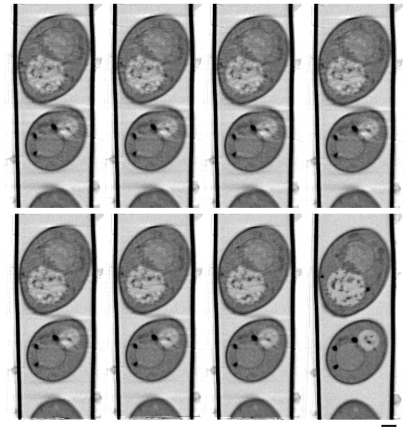
Othoslices along the rotation axis through the reconstruction using different numbers of iterations of projection matching. Number of iterations, top: 2, 5, 10, 25 (left to right); bottom 50, 75, 100 (left to right) and manual alignment (bottom, far right). Scale bar = 1 um.
Finally we compare reconstruction quality in manual alignment and AREC3D alignment using a noise compensated leave one out method. In this method, reconstructions are calculated based on a projection stack with one projection angle missing. An approximation to the deleted projection is generated from the reconstructed volume and compared to the original, omitted projection using standard FRC methods (Saxton and Baumeister, 1982). This process is repeated every ten images and the results are averaged, as shown in Figure 8. For the microscope settings used for data collection in this work (32 nm pixel size), and with a FRC threshold of 0.5, the resolution obtained for the different reconstruction methods is 87 nm for the manually aligned data and 94 nm for the AREC3D aligned data. Despite some differences in the y-shifts and in-plane rotations, the overall quality of the reconstruction obtained using AREC3D is satisfactory for data analysis (e.g. segmentation). For analyses requiring the best resolution or optimized contrast the AREC3D derived alignment parameters can be used as the initial input to a more thorough analysis procedure. For instance, with human intervention “bad” projections caused by an uncontrolled seismic noise could be removed from the data prior to alignment, leading to improvement over automatic procedures.
Figure 8.

Comparison of Fourier ring correlation (FRC) curves calculated with the leave-on-out method (data has 32 nm pixel size). The dotted line indicates the 0.5 threshold. Manual alignment shows slightly better results than AREC3D automatic alignment with 100 iterations.
Discussion
Development and implementation of the AREC3D software package are significant steps forward for high throughput soft x-ray tomography. Tight integration of automatic alignment and tomographic reconstruction has enabled investigators using SXT at the NCXT to obtain almost real-time feedback on the data as it is being collected using only a few iterations of projection matching in AREC3D. An increased number of iterations can be used for later refinement. The prompt reconstructions obtained using AREC3D are invaluable to investigators performing SXT experiments; by using binned images rather than full-resolution images, reconstructions could be obtained even more quickly. The ability to obtain high-resolution cellular tomograms while examining a large number of cells under different conditions enables intelligent decision making during the experiment.
In many cases, the volumes obtained after convergence of the algorithm are sufficient for further processing; in some cases, they are of sufficient quality to allow selection of a few data sets that can be reconstructed using fiducial markers to get improved resolution. SXT image processing will continue to leverage off state-of-the-art developments in electron tomography, but the unique ability to examine large numbers of cells, and the enormously relaxed demands on specimen geometry, makes it necessary to develop new software optimized for SXT.
AREC3D is a small but significant component of an automated data analysis pipeline for high-throughput SXT. As the number of biological soft x-ray microscopy facilities increases (Pereiro et al., 2009), there will be many additional creative contributions to the portfolio of software tailored to SXT. New software is required for virtually every aspect of the SXT data processing pipeline, from the difficult problem of automatic segmentation to data knowledge bases (DOE, 2010) for archiving and mining the unique data obtained with SXT and with correlated high N.A cryolight fluorescence microscopy (McDermott et al., 2009).
Acknowledgments
This work was funded by the Department of Energy Office of Biological and Environmental Research Grant DE-AC0 5CH11231 and the NIH National Center for Research Resources Grant RR019664.
Footnotes
Publisher's Disclaimer: This is a PDF file of an unedited manuscript that has been accepted for publication. As a service to our customers we are providing this early version of the manuscript. The manuscript will undergo copyediting, typesetting, and review of the resulting proof before it is published in its final citable form. Please note that during the production process errors may be discovered which could affect the content, and all legal disclaimers that apply to the journal pertain.
References
- Agulleiro JI, Fernandez JJ. Fast tomographic reconstruction on multicore computers. Bioinformatics. 2011;27:582–583. doi: 10.1093/bioinformatics/btq692. [DOI] [PubMed] [Google Scholar]
- Amat F, Moussavi F, Comolli LR, Elidan G, Downing KH, Horowitz M. Markov random field based automatic image alignment for electron tomography. J Struct Biol. 2008;161:260–275. doi: 10.1016/j.jsb.2007.07.007. [DOI] [PubMed] [Google Scholar]
- Amat F, Castano-Diez D, Lawrence A, Moussavi F, Winkler H, Horowitz M. Alignment of Cryo-Electron Tomography Datasets. Method Enzymol. 2010;482:343–367. doi: 10.1016/S0076-6879(10)82014-2. [DOI] [PubMed] [Google Scholar]
- Attwood DT. Soft x-rays and extreme ultraviolet radioation: principles and applications. Cambridge University Pres; New York: 1999. [Google Scholar]
- Brandt SS. Markerless Alignment in Electron Tomography. In: Frank J, editor. Electron Tomography. 2. Springer; New York, NY: 2006. pp. 187–215. [Google Scholar]
- Cardone G, Grunewald K, Steven AC. A resolution criterion for electron tomography based on cross-validation. J Struct Biol. 2005;151:117–129. doi: 10.1016/j.jsb.2005.04.006. [DOI] [PubMed] [Google Scholar]
- Carrascosa JL, Chichon FJ, Pereiro E, Rodriguez MJ, Fernandez JJ, Esteban M, Heim S, Guttmann P, Schneider G. Cryo-X-ray tomography of vaccinia virus membranes and inner compartments. J Struct Biol. 2009;168:234–239. doi: 10.1016/j.jsb.2009.07.009. [DOI] [PubMed] [Google Scholar]
- Castano-Diez D, Seybert A, Frangakis AS. Tilt-series and electron microscope alignment for the correction of the non-perpendicularity of beam and tilt-axis. J Struct Biol. 2006;154:195–205. doi: 10.1016/j.jsb.2005.12.009. [DOI] [PubMed] [Google Scholar]
- Castano-Diez D, Scheffer M, Al-Amoudi A, Frangakis AS. Alignator: A GPU powered software package for robust fiducial-less alignment of cryo tilt-series. J Struct Biol. 2010;170:117–126. doi: 10.1016/j.jsb.2010.01.014. [DOI] [PubMed] [Google Scholar]
- Castano-Diez D, Moser D, Schoenegger A, Pruggnaller S, Frangakis AS. Performance evaluation of image processing algorithms on the GPU. J Struct Biol. 2008a;164:153–160. doi: 10.1016/j.jsb.2008.07.006. [DOI] [PubMed] [Google Scholar]
- Castano-Diez D, Al-Amoudi A, Glynn AM, Seybert A, Frangakis AS. Fiducial-less alignment of cryo-sections (Reprinted from J. Struct Biol., vol 159, pg 413–423, 2007) J Struct Biol. 2008b;161:249–259. doi: 10.1016/S1047-8477(08)00060-9. [DOI] [PubMed] [Google Scholar]
- Chen H, Hughes DD, Chan TA, Sedat JW, Agard DA. IVE (Image Visualization Environment): A software platform for all three-dimensional microscopy applications. J Struct Biol. 1996;116:56–60. doi: 10.1006/jsbi.1996.0010. [DOI] [PubMed] [Google Scholar]
- Diez DC, Seybert A, Frangakis AS. Tilt-series and electron microscope alignment for the correction of the non-perpendicularity of beam and tilt-axis. J Struct Biol. 2006;154:195–205. doi: 10.1016/j.jsb.2005.12.009. [DOI] [PubMed] [Google Scholar]
- DOE, U.S; U. S. D. o. E. O. o. Science Systems Biology Knowledgebase Implementation Plan. 2010. [Google Scholar]
- Fernandez JJ. High performance computing in structural determination by electron cryomicroscopy. J Struct Biol. 2008;164:1–6. doi: 10.1016/j.jsb.2008.07.005. [DOI] [PubMed] [Google Scholar]
- Fessler JA. Hybrid Poisson/polynomial Objective Functions for Tomographic Image Reconstruction from Transmission Scans. IEEE Transactions on Image Processing. 1995;4:1439–1450. doi: 10.1109/83.465108. [DOI] [PubMed] [Google Scholar]
- Fessler JA. ASPIRE3.0 User’s Guide: A Sparse Iterative Reconstruction Libray Technical Report Communications and Signal Processing Laboratory. The University of Michigan; Ann Arbor: 2009. [Google Scholar]
- Frank J. Electron Tomography Methods for Three-Dimensional Visualization of Structures in the Cell. 2. Springer; 2006. [Google Scholar]
- Hansen PC. Rank-deficient and Discrete Ill-posed Problems: Numerical Aspects of Linear Inversion SIAM. 1998. [Google Scholar]
- Harris C, Stephens M. A combined corner and edge detector. Proceedings of the 4th Alvey Vision Conference; 1988. pp. 147–151. [Google Scholar]
- Houben L, Bar Sadan M. Refinement procedure for the image alignment in high-resolution electron tomography. Ultramicroscopy. 2011;111:1512–1520. doi: 10.1016/j.ultramic.2011.06.001. [DOI] [PubMed] [Google Scholar]
- Kremer JR, Mastronarde DN, McIntosh JR. Computer Visualization of Three-Dimensional Image Data Using IMOD. J Struct Biol. 1996;116:71–76. doi: 10.1006/jsbi.1996.0013. [DOI] [PubMed] [Google Scholar]
- Le Gros MA, McDermott G, Larabell CA. X-ray tomography of whole cells. Current Opinion in Structural Biology. 2005;15:593–600. doi: 10.1016/j.sbi.2005.08.008. [DOI] [PubMed] [Google Scholar]
- Liu Y, Penczek PA, Mcewen BF, Frank J. A Marker-Free Alignment Method for Electron Tomography. Ultramicroscopy. 1995;58:393–402. doi: 10.1016/0304-3991(95)00006-m. [DOI] [PubMed] [Google Scholar]
- Mastronarde DN. Correction for non-perpendicularity of beam and tilt axis in tomographic reconstructions with the IMOD package. J Microsc-Oxford. 2008;230:212–217. doi: 10.1111/j.1365-2818.2008.01977.x. [DOI] [PubMed] [Google Scholar]
- McDermott G, Le Gros MA, Knoechel CG, Uchida M, Larabell CA. Soft X-ray tomography and cryogenic light microscopy: the cool combination in cellular imaging. Trends in Cell Biology. 2009;19:587–595. doi: 10.1016/j.tcb.2009.08.005. [DOI] [PMC free article] [PubMed] [Google Scholar]
- Meyer-Ilse W, Hamamoto D, Nair A, Lelievre SA, Denbeaux G, Johnson L, Pearson AL, Yager D, Legros MA, Larabell CA. High resolution protein localization using soft X-ray microscopy. J Microsc-Oxford. 2001;201:395–403. doi: 10.1046/j.1365-2818.2001.00845.x. [DOI] [PubMed] [Google Scholar]
- Pacheco PS. An Introduction to Parallel Programming. 1. Morgan Kauffmann; Waltham, Massachusetts: 2011. [Google Scholar]
- Penczek PA, Grassucci RA, Frank J. The Ribosome at Improved Resolution - New Techniques for Merging and Orientation Refinement in 3d Cryoelectron Microscopy of Biological Particles. Ultramicroscopy. 1994;53:251–270. doi: 10.1016/0304-3991(94)90038-8. [DOI] [PubMed] [Google Scholar]
- Pereiro E, Nicolas J, Ferrer S, Howells MR. A soft X-ray beamline for transmission X-ray microscopy at ALBA. Journal of Synchrotron Radiation. 2009;16:505–512. doi: 10.1107/S0909049509019396. [DOI] [PubMed] [Google Scholar]
- Saxton WO, Baumeister W. The Correlation Averaging of a Regularly Arranged Bacterial-Cell Envelope Protein. J Microsc-Oxford. 1982;127:127–138. doi: 10.1111/j.1365-2818.1982.tb00405.x. [DOI] [PubMed] [Google Scholar]
- Schneider G, Guttmann P, Heim S, Rehbein S, Mueller F, Nagashima K, Heymann JB, Muller WG, McNally JG. Three-dimensional cellular ultrastructure resolved by X-ray microscopy. Nat Methods. 2010;7:985–U116. doi: 10.1038/nmeth.1533. [DOI] [PMC free article] [PubMed] [Google Scholar]
- Sorzano COS, Marabini R, Velazquez-Muriel J, Bilbao-Castro JR, Scheres SHW, Carazo JM, Pascual-Montano A. XMIPP: a new generation of an open-source image processing package for electron microscopy. J Struct Biol. 2004;148:194–204. doi: 10.1016/j.jsb.2004.06.006. [DOI] [PubMed] [Google Scholar]
- Sorzano COS, Messaoudi C, Eibauer M, Bilbao-Castro JR, Hegerl R, Nickell S, Marco S, Carazo JM. Marker-free image registration of electron tomography tilt-series. Bmc Bioinformatics. 2009:10. doi: 10.1186/1471-2105-10-124. [DOI] [PMC free article] [PubMed] [Google Scholar]
- Streibl N. Three-dimensional imaging by a microscope. J Opt Soc Am A. 1985;2:121–127. [Google Scholar]
- Uchida M, McDermott G, Wetzler M, Le Gros MA, Myllys M, Knoechel C, Barron AE, Larabell CA. Soft X-ray tomography of phenotypic switching and the cellular response to antifungal peptoids in Candida albicans. Proceedings of the National Academy of Sciences of the United States of America. 2009;106:19375–19380. doi: 10.1073/pnas.0906145106. [DOI] [PMC free article] [PubMed] [Google Scholar]
- Uchida M, Sun Y, McDermott G, Knoechel C, Le Gros MA, Parkinson D, Drubin DG, Larabell CA. Quantitative analysis of yeast internal architecture using soft X-ray tomography. Yeast. 2011;28:227–236. doi: 10.1002/yea.1834. [DOI] [PMC free article] [PubMed] [Google Scholar]
- Weiss D, Schneider G, Niemann B, Guttmann P, Rudolph D, Schmahl G. Computed tomography of cryogenic biological specimens based on X-ray microscopic images. Ultramicroscopy. 2000;84:185–197. doi: 10.1016/s0304-3991(00)00034-6. [DOI] [PubMed] [Google Scholar]
- Winkler H, Taylor KA. Accurate marker-free alignment with simultaneous geometry determination and reconstruction of tilt series in electron tomography. Ultramicroscopy. 2006;106:240–254. doi: 10.1016/j.ultramic.2005.07.007. [DOI] [PubMed] [Google Scholar]
- Xu W, Xu F, Jones M, Keszthelyi B, Sedat J, Agard D, Mueller K. High-performance iterative electron tomography reconstruction with long-object compensation using graphics processing units (GPUs) J Struct Biol. 2010;171:142–153. doi: 10.1016/j.jsb.2010.03.018. [DOI] [PMC free article] [PubMed] [Google Scholar]
- Yang C, Ng EG, Penczek PA. Unified 3-D structure and projection orientation refinement using quasi-Newton algorithm. J Struct Biol. 2005;149:53–64. doi: 10.1016/j.jsb.2004.08.010. [DOI] [PubMed] [Google Scholar]
- Zheng SQ, Keszthelyi B, Branlund E, Lyle JM, Braunfeld MB, Sedat JW, Agard DA. UCSF tomography: An integrated software suite for real-time electron microscopic tomographic data collection, alignment, and reconstruction. J Struct Biol. 2007;157:138–147. doi: 10.1016/j.jsb.2006.06.005. [DOI] [PubMed] [Google Scholar]