Spin Dephasing Under Nonlinear Gradients: Implications for Imaging and Field Mapping

Abstract

This work examines the prototypical MR echo that would be expected for a voxel of spins evolving in a strong nonlinear field, specifically focusing on the quadratic z²-½(x²+y²) field. Dephasing under nonlinear gradients is increasingly relevant given the growing interest in nonlinear imaging, and here we report several notable differences from the linear case. Most notably, in addition to signal loss, intravoxel dephasing under gradients creating a wide and asymmetric frequency distribution across the voxel can cause skewed and nonlinear phase evolution. After presenting the qualitative and analytical origins of this difference, we experimentally demonstrate that neglecting these dynamics can lead to significant errors in sequences that assume phase evolution is proportional to voxel frequency, such as those used for field mapping. Finally, simplifying approximations to the signal equations are presented, which not only provide more intuitive forms of the exact expression, but also result in simple rules to predict key features of the nonlinear evolution.

Introduction

Imaging techniques employing nonlinear gradients have received increasing interest for a number of reasons. They may allow imaging with lower dB/dt to decrease the possibility of peripheral nerve stimulation (1). It has already been demonstrated that nonlinear encoding strategies using multidimensional coil arrays can lead to better reconstruction of highly undersampled images (2). Furthermore, the spatially varying resolution of these encoding fields can be exploited to improve resolution specifically over a particular region of interest (3), (4), and higher-order field shapes provide denser encoding at the periphery, where surface coil sensitivity is highest. Finally, these shapes can be used to create artificial effective RF coil profiles that efficiently supplement skipped data from standard imaging trajectories, such as Cartesian or radial encoding methods (5).

This paper explores some of the basic dynamics of spins evolving under strong nonlinear fields, particularly our experimentally available z² - ½(x²+y²) field. The prototypical MR signal emanating from a boxcar of spins evolving under a linearly varying magnetic field, henceforth called a linear gradient, is a basic and familiar result. Namely, the magnitude evolves as a sinc function whose argument is proportional to the frequency range across the boxcar. The phase of the signal is independent of this frequency range and changes linearly with time, with a frequency that depends only on the center of the boxcar. However, the signal from an object evolving in a quadratic field leads not only to decreased signal intensity, but also to nonlinear phase evolution. Interpreting this dephasing-based evolution as a Larmor precession can lead to important consequences either for calibrating nonlinear imaging gradients or for other standard experiments that map nonlinear fields by equating phase evolution with frequency, such as those routinely used to calibrate gradient strengths (6) and measure eddy currents (7). Furthermore, the encoding matrices often used to reconstruct nonlinearly encoded images typically assume that a voxel’s contribution to the bulk signal has a phase that is proportional to time. If these voxels are square and the nonlinearity of the field across them is strong enough to create an asymmetric frequency distribution, the phase evolution of the voxel is generally nonlinear with time, so this encoding matrix would be inaccurate and artifacts would appear in the reconstructed image..

The outline of this report is as follows. Section II examines the exact analytical expression for the bulk magnetization as it evolves in a quadratic gradient. We show that intravoxel gradient dephasing, which is normally associated only with signal loss, can distort phase evolution and affect a voxel’s apparent frequency. In Section III, we demonstrate these distortions experimentally, comparing gradient maps taken at different slice thicknesses and offsets, which show good agreement with the analytical expression. Section IV attempts to give a more intuitive picture of the exact expression for S(t) by presenting approximations that reduce the dynamics to analogs of the classic sinc form. Section V recapitulates the major findings and concludes.

Analytical Model

Most introductions to magnetic resonance imaging lead into the standard gradient echo by considering the ideal echo for a one-dimensional boxcar of spin density evolving under a linear z-gradient. Namely, it is:

$$S_l(t)=\iint {\int }_{z_1}^{z_2}\delta (x_0)\delta (y_0)e^{-i\gamma G_{z}tz}\mathit{dzdydx}=e^{-i\gamma {\mathit{Gtz}}_0}\frac{-2sin(\gamma Gt\mathrm{\Delta }z)}{\gamma Gt}$$ [1]

where z₁ = z₀-Δz and z₂ = z₀+Δz (7,8). δ(s) in this expression is the Kroenecker delta function, and we have taken x₀ and y₀ as isocenter so that integration over these dimensions is unity. As previously noted, the phase evolves linearly with time, and the magnitude envelope follows a sinc function. Exact nulls occur at t=(2γGΔz)⁻¹=(Δω)⁻¹, when the range of phases across the boxcar covers a multiple of 2π.

For evolution under the three dimensional z² - ½(x²+y²) hyperboloid field, the ideal echo can be similarly derived for a one dimensional box car of spins (with point like dimensions along x and y).

$$S_q(t)={\iiint }_{z_1}^{z_2}\delta (x_0)\delta (y_0)e^{-i\gamma G_{z^2}t\left(z^2-\frac{1}{2}(x^2+y^2)\right)}\mathit{dzdydx}$$ [2]

$$=\sqrt{\frac{1}{4i\gamma Gt}}\{\text{erf}(\sqrt{i\gamma Gt}{z}_2)-\text{erf}(\sqrt{i\gamma Gt}{z}_1)\}{e}^{i\gamma G_{z^2}t\left(\frac{1}{2}(x_0^2+y_0^2)\right)}$$ [3]

where erf(x) is the Gauss error function. Though this expression is undefined at t=0, it is physically clear that S_q(t=0)=M₀ (9). The resulting signal can be interpreted as the signal from a voxel with point-like area in x and y, but non-negligible thickness in the slice direction. In this limit, the x and y positions simply lead to a familiar frequency shift of the signal. Thus we take these to be zero and focus on dynamics arising from the finite width along z¹.

In Figure 1, we simulate the signal described in Eq. [3] for various slice thicknesses and offsets from isocenter. These figures use a gradient of 2kHz/cm², meaning that the frequency offset at a given (x₀,y₀,z₀) is equal to 2(z₀² - ½(x₀²+y₀²))kHz. Figure 1a shows the phase evolution as a function of time for slices of various thickness, but all centered at isocenter. For vanishingly thin slices (blue line) the phase is constant over time, as would be expected for a voxel at isocenter and on resonance. However, at larger thicknesses, the voxel has a nonlinear phase evolution that mimics a nonlinear Larmor evolution. The most salient evolution occurs as the signal phase sweeps through the peak of the echo, and it can be physically attributed to the unique symmetry of the quadratic gradient field across z=0. In the moments just after the peak of the echo, the spins both above and below the isocenter are all moving in the same direction. This shifts the phase of the bulk magnetization causing phase precession of the bulk signal. This is in sharp contrast to the dynamics under a linear gradient field, where there is antisymmetry about the center of the slice. In the linear case, evolution by those spins above the slice center is counterbalanced by evolution of the spins below it, so no coherent precession of the bulk is observed.

Figure 1. Signal Evolution of a One Dimensional Voxel.

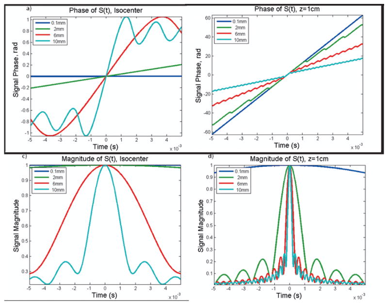
Through slice dephasing under a z² -½(x²+y²) field can lead to phase evolution of the bulk signal, even for a slice at isocenter where evolution would not be expected (1a). For slices away from isocenter, this evolution can dramatically impact the apparent phase slope of the voxel, thus distorting its apparent frequency (1b). Through plane dephasing is also seen to impact the magnitude envelope of the signal (1c–d), though certain sinc-like features are preserved.

These deviations from linearity become significantly more pronounced as we consider slices away from isocenter, as Figure 1b shows (different scale) for the phase evolution observed for a slice at z=1cm. In these figures, regularities in the evolution become more apparent, and it is seen that significant deviations from linearity occur with a period t=1/Δω_z, where Δω_z is the frequency range across the slice thickness. Furthermore, the overall apparent frequency of this voxel differs dramatically as a function of the slice thickness, which could cause serious errors in gradient field mapping. In general, the through-plane dephasing causes the apparent frequency to shift toward lower frequencies. This can be qualitatively explained by noting that, assuming |z₁|< |z₂|, the frequency bins become spatially narrower as they go from z₁ to z₂. Thus, for a sample of uniform density, there are more spins at frequencies near z₁ than near z₂, and these slower frequencies dominate the signal. We also show the magnitude envelopes that correspond to these signals, both at isocenter (Figure 1c) and at z=1cm (Figure 1d). From these plots, we can note that the off center magnitude envelope does bear some similarity to the sinc expected from linear dephasing. For example, though the signal does not go through a true null, it does have characteristic minima occurring at t=n/Δω_z.

Finally we simulate how these results are expected to affect the signal from a realistic single slice phantom. We simulate the signal from the numerical phantom shown in Figure 2a evolving in a three dimensional z² - ½(x²+y²) gradient of 2kHz/cm² at z=3cm, and Figures 2b and 2c show the phase and magnitude of the echoes with varying slice thickness.

Figure 2. Signal Evolution of a Three Dimensional Slice.

The phantom (FOV=6cm) used to simulate signal from a three dimensional slice centered at z=1cm is shown in panel a. For very thin slices (blue), the phase, magnitude, and transform of the signal are similar to the line, sinc, and tophat that would respectively be predicted from an infinitely thin disk. As the slice gets larger, the phase and magnitude plots exhibit the features noted in Figure 1. Furthermore, the transform of these signals becomes lopsided, as well as broadened, reflecting the asymmetric distribution of frequency bins across the rectangular slice.

Though our simulations are performed on a more realistic, structured phantom, the object is roughly circular, and we can approximate the signal from a negligibly thin slice (blue line) as: [4]

$$S_q(t)={\iiint }_0^r\delta (z_0)e^{-i\gamma G_{z^2}t\left(z^2-\frac{1}{2}(r^2)\right)}\mathit{rdrdzd}\theta$$ [4]

As previously reported (2), this integral is of the form e^udu,u=r², and is mathematically equivalent to the integral of a square shape under linear gradients. Thus, it results in the familiar sinc(Δω_rt), where Δω_r is the range of frequencies along the radial direction, and minima occur at r=1/Δω_r. At the other end of the spectrum, we can look at the thickest slices, where Δω_z is greater than Δω_r. Here, the through-plane dephasing appears to dominate, and the minima occur near t=1/Δω_z. Intermediate cases fall between these.

Finally, panel 2d examines the Fourier transform of these signals. The transforms of very thin slices, whose echoes closely resemble sinc functions, are unsurprisingly similar to top hats. However, as we begin integrating over a finite slice thickness in the z-direction, the projections not only broaden, but also become asymmetric. This is yet another consequence of the frequency bins being spatially narrower as they go from z₁ to z₂, thus reducing the intensity at each frequency bin in the transform domain.

Experimental Consequences

One clear example of how this nonlinearity can affect even routine experiments is in a standard field mapping experiment. Field maps were generated by inserting a nonlinear gradient pulse into the echo time of a FLASH sequence, incrementing the flat top time of the nonlinear gradient pulse on subsequent images, and fitting the resulting phase progression to a line. In the linear case, intravoxel dephasing should not change the unwrapped phase progression of the voxel, whereas we have shown that it can significantly affect a voxel’s phase under a quadratic gradient.

Images were collected on a 3.0-T Siemens Trio human magnet (Erlangen, Germany) equipped with an actively-shielded 12-cm insert coil (Resonance Research Inc., MA) able to generate the z² -½(x²+y²) spherical harmonic at strengths up to 18 kHz/cm², though the presented field maps were generated for a field of 450Hz/cm² over a 10cm FOV, TE/TR=10/100ms. In the acquired images, the in-plane resolution is high enough (.7mm/pixel) that intravoxel dephasing along the transverse direction can be neglected, but the through-plane dimension is not usually as small. Thus, each voxel in the image behaves much like the rod of infinitesimal area that is simulated in Figure 1. While magnitude modulations due to intravoxel dephasing, as well as their recovery, have been thoroughly examined elsewhere (10–15), we highlight that, even when imaging is performed with linear gradients, the phase of the reconstructed image can be significantly affected by nonlinear fields. This can have serious consequences for imaging techniques that rely on phase, and particularly for those that linearly equate phase evolution with frequency, such as frequency mapping.

The first row of Figure 3 shows a slice at isocenter, with 3a displaying a magnitude image and 3b displaying the frequency map for a 1cm thick slice. Panels 3c–f show the bias in the observed frequency as the slice thickness is increased to 4, 6, 8 and 10mm, and it is imperceptible. This corroborates the predictions of Figure 1a for a slice at isocenter: aside from a jump near t=0, the phase of the signal at isocenter is minimally affected by through-slice dephasing. Off isocenter, however, we see a significant bias in the frequency maps 3i–l, which is also in qualitative agreement with our simulations (Figure 1b).

Figure 3. Slice Thickness Affects Frequency Maps.

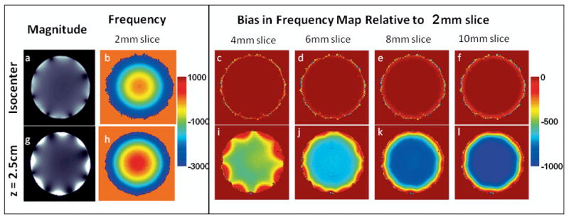
With linear gradients, the slice thickness would not be expected to affect the frequency map generated by a standard field mapping sequence. In our uniform phantom (a), the slice at isocenter yields the same frequency map (b) for the z²-½(x²–y²) gradient regardless of slice thickness. There is no bias introduced as the slice is widened to 4, 6, 8, or 10mm (c–f). However, at z=2.5cm (g), the analytical expression predicts that phase evolution from intravoxel dephasing becomes significant. If this evolution is interpreted as evolution of the bulk, the observed frequency of the slice becomes a function of the slice thickness (h–l). A linear fit to the exact expression in Eq. [3] predicts biases of −100, −400, −550, −900Hz for these thicknesses, in good agreement with the data.

Finally, we examine how thin a slice must be such that its apparent evolution actually reflects the frequency we would normally associate with that slice, i.e. the frequency at its center. The answer greatly depends on the offset of the slice, as shown in Figure 4. This plot shows that the effect is most pronounced in slices where there is a large frequency range across the voxel in some direction, either because of a large offset, a large slice thickness, or both of these. In the next section, we derive a more quantitative formulation of this rule of thumb.

Figure 4. Apparent Frequency.

The apparent frequency depends on both the position of the slice center and also its thickness. Apparent frequencies were calculated by applying a linear fit to the phases simulated over 1ms of evolution under a 1.5kHz/cm² hyperboloid field.

Approximate Solutions

We now return to the analytical expression for a voxel of infinitely small area and finite slice thickness to consider simplifying approximations. For slices near isocenter and times near zero, the argument of the error functions in Eq. [3] are small, and a Taylor expansion is appropriate.

Applying the two term expansion, $\text{erf}(x)\approx \frac{2}{\sqrt{\pi }}[x-\frac{x^2}{3}]$, to Eq. [2] yields:

$$S_q(t)\approx (z_2-z_1)-\frac{i\gamma Gt(z_2^3-z_1^3)}{3}.$$ [5]

Thus, near zero, the phase should follow

$${\mathit{tan}}^{-1}\left\{\frac{i\gamma G(z_2^3-z_1^3)}{3(z_2-z_1)}t\right\},$$ [6]

and the phase slope of the signal near t=0 is

$$\left\{\frac{i\gamma G(z_2^3-z_1^3)}{3(z_2-z_1)}t\right\}\frac{1}{1+t^2}.$$ [7]

For slices at isocenter, this would predict an initial frequency proportional to Δz², which is precisely what is observed in the linear portions of Figure 1a.

For large offsets, we can revisit the integral in Eq. [2]. Multiplying by $\frac{-2i\gamma G_{z^2}tz}{-2i\gamma G_{z^2}tz}$, we can integrate by parts:

$$S_q(t)={\int }_{z_1}^{z_2}\{\frac{1}{2i\gamma G_{z^2}tz}\}\{(-2i\gamma G_{z^2}tz)e^{-i\gamma G_{z^2}{tz}^2}\}dz$$ [8]

$$={\frac{-1}{2i\gamma G_{z^2}tz}\{e^{-i\gamma G_{z^2}{tz}^2}\}|}_{z_2}^{z_1}-{\int }_{z_1}^{z_2}\frac{1}{2i\gamma G_{z^2}{tz}^2}\{e^{-i\gamma G_{z^2}{tz}^2}\}dz.$$ [9]

For large values of G_z²tz², the second integral can be dropped since

$$S_q(t)={\int }_{z_1}^{z_2}\{e^{-i\gamma G_{z^2}{tz}^2}\}dz\gg {\int }_{z_1}^{z_2}\frac{1}{2i\gamma G_{z^2}{tz}^2}\}\{e^{-i\gamma G_{z^2}{tz}^2}\}dz.$$ [10]

This is equivalent to an asymptotic expansion of the error functions in the exact solution of the integral. (16) It yields:

$$S_q(t)\approx \frac{1}{2i(\gamma G_{z^2}{z}_1{z}_2)t}\{z_1{e}^{-i{\omega }_q(z_2)t}-z_2{e}^{-i{\omega }_q(z_1)t}\}.$$ [11]

Where we have incorporated the fact that γG_z²z² − ω_q(z), the frequency at z under a quadratic gradient. Note this already bears striking similarity to the standard sinc function, which can be written as:

$$S_l(t)=\frac{i}{\gamma G_{z}t}\{e^{-i{\omega }_l(z_2)t}-e^{-i{\omega }_l(z_1)t}\}$$ [12]

where we have similarly rewritten the frequency at a given z under a linear gradient as ω_l(z). To further the connections between Eq. [12] and the sinc form of Eq. [1], we can define ${\omega }_{0,q}=\frac{{\omega }_q(z_2)+{\omega }_q(z_1)}{2}$ and Δω_q = ω_q(z₂) − ω_q(z₁). Note that this definition fundamentally differs from the linear case in that ω_0,q ≠ ω_q(z₀); it is shifted towards ω_q(z₂).

$$S_q(t)\approx \frac{-e^{-i{\omega }_{0,q}t}}{\gamma G_{z^2}(z_0^2-{(\mathrm{\Delta }z)}^2)t}\left\{z_{0}sin\left(\frac{\mathrm{\Delta }{\omega }_{q}t}{2}\right)-i\mathrm{\Delta }\mathit{zcos}\left(\frac{\mathrm{\Delta }{\omega }_{q}t}{2}\right)\right\}.$$ [13]

When Δz is small and the second term can be neglected, this expression is essentially a sinc magnitude envelope with a linear phase slope of ω_0,q. However, as Δ_z becomes significant, it is more appropriate to view this as the product of two vectors: one that traces out a circle at a rate of ω_0,q and one that describes precession around an ellipse with major and minor axes of z₀ and Δz, respectively. The phase of the product, i.e. of S_q(t), is simply:

$${\omega }_{0,q}t+{\mathit{tan}}^{-1}\{\frac{\mathrm{\Delta }\mathit{zcos}(\mathrm{\Delta }{\omega }_{q}t/2)}{z_{0}sin(\mathrm{\Delta }{\omega }_{q}t/2)}\}$$ [14]

This explains several of the features observed in Figure 1b. The second term contains the nonlinearity, which is periodic and repeats every $\frac{1}{\mathrm{\Delta }{\omega }_q}$. Furthermore, the phase of a linear frequency precession over an ellipse, (simulated in Figure 5), qualitatively matches the observed nonlinearities in the phase, changing very quickly near the minor axis and very slowly near the major axis.

Figure 5. Phase Evolution of Elliptical Precession.

In the asymptotic limit (Eq. [14]), the nonlinear component of the phase evolution under a z²-(x²+y²) gradient can be described by precession about an ellipse. Here, we simulate just the nonlinear component of the phase evolution that would be expected for a slice centered at z=3cm evolving under a 100Hz/cm² field.

With this approximation, we can justify a simplified rule of thumb for the observed frequency in a gradient mapping experiment. The observed phase precession will be ω_0,q with an additional -π accruing (nonlinearly) every $\frac{1}{\mathrm{\Delta }{\omega }_q}$. This rule of thumb should be used with caution since it depends on describing a nonlinear but periodic phase progression as a linear phase slope². However, for our experimental frequency maps (Figure 3), such a calculation would predict observed frequency biases of −300, −650, −900 and −1200Hz, which is in reasonable agreement with the observed shifts. We can also use this rule of thumb to roughly estimate the impact of weaker nonlinear gradients, like those that might be encountered due to susceptibility gradients or poor shim. For example, at 1cm off isocenter with a gradient of 50Hz/cm², this model would predict observed frequencies of 50, 39, 29, 21, 14, and 8Hz if the dimensions along the quadratic field are 0.1, 2, 4, 6, 8 and 10mm, respectively, assuming we fit the phase over a large range of timepoints. If a smaller range of timepoints is taken (<1/Δω_z) and the nonlinear region of phase evolution happens to be avoided, the apparent evolution will approach ω_0,q, which is 50, 51, 53, 56, 62 and 68Hz, respectively.

Conclusion

In conclusion, we have examined both the phase and magnitude of echoes resulting from evolution under a quadratic z²-½(x²+y²) gradient with both numerical simulations and analytical derivations. We have analyzed its impact on the standard gradient mapping experiment and shown that, because of the three dimensional nature of the gradient, slice thickness can significantly impact the observed frequency in the slice. Finally, we presented several approximations that can be used to estimate the impact of this through-slice dephasing and verified their agreement with our own experimental findings.

More broadly, this report highlights that intravoxel dephasing under nonlinear gradients leads not only to a signal loss, but also to complex phase behavior. Whenever the frequency distribution across the voxel is asymmetric, the observed phase evolution is nonlinear, and care should be taken when assuming that the frequency of the voxel is proportional to the observed phase change. While this paper follows the precise dynamics of the z²-½(x²+y²) field, we can expect these effects to be present in any case where there is a significant and asymmetric frequency spread across the voxel. As an example, this correction may be of value to susceptibility weighted imaging studies, which begin with field maps that assume phase is a linear function of time, even though it is known that the intravoxel fields are generally nonlinear. Quantifying the nonlinearity of the phase evolution may provide another parameter to characterize the susceptibility variations within a voxel (17,18).

References

- 1.Hennig J, Welz AM, Schultz G, Korvink J, Liu Z, Speck O, Zaitsev M. Parallel imaging in non-bijective, curvilinear magnetic field gradients: a concept study. MAGMA. 2008;21:5–14. doi: 10.1007/s10334-008-0105-7. [DOI] [PMC free article] [PubMed] [Google Scholar]
- 2.Stockmann JP, Ciris PA, Galiana G, Tam L, Constable RT. O-space imaging: Highly efficient parallel imaging using second-order nonlinear fields as encoding gradients with no phase encoding. Magn Reson Med. 2010;64(2):447–56. doi: 10.1002/mrm.22425. [DOI] [PMC free article] [PubMed] [Google Scholar]
- 3.Gallichan D, Cocosco CA, Dewdney A, Schultz G, Welz A, Hennig J, Zaitsev M. Simultaneously driven linear and nonlinear spatial encoding fields in MRI. Magn Reson Med. 2011 doi: 10.1002/mrm.22672. [Epub ahead of print] [DOI] [PubMed] [Google Scholar]
- 4.Schultz G, Ullmann P, Lehr H, Welz AM, Hennig J, Zaitsev M. Reconstruction of MRI data encoded with arbitrarily shaped, curvilinear, nonbijective magnetic fields. Magn Reson Med. 2010;64(5):1390–403. doi: 10.1002/mrm.22393. [DOI] [PubMed] [Google Scholar]
- 5.Galiana G, Stockman HS, Constable RT. Enhanced Parallel Imaging Acceleration with a B1 Accelerated Reconstruction Sequence (BARS). Proceedings of the 18th Annual Meeting of ISMRM; Stockholm, Sweden. 2010. p. 2850. [Google Scholar]
- 6.Jezzard P, Barnett AS, Pierpaoli C. Characterization of and correction for eddy current artifacts in echo planar diffusion imaging. Magn Reson Med. 2005;39(5):801–812. doi: 10.1002/mrm.1910390518. [DOI] [PubMed] [Google Scholar]
- 7.Haacke M, Brown RW, Thompson MR, Venkatesan R. Magnetic resonance imaging: Physical principles and sequence design. New York: John Wiley & Sons; 1999. [Google Scholar]
- 8.De Graaf RA. In vivo NMR spectroscopy: principles and techniques. Chichester, UK: John Wiley & Sons; 2008. [Google Scholar]
- 9.Abramowitz M, Stegun IA. Handbook of Mathematical Functions with Formulas, Graphs, and Mathematical Tables. 10. New York: Dover Publications; 1972. p. 303. [Google Scholar]
- 10.Young IR, Cox IJ, Bryant DJ, Bydder GM. The benefits of increasing spatial resolution as a means of reducing artifacts due to field inhomogeneities. Magn Reson Imaging. 1988;6(5):585–90. doi: 10.1016/0730-725x(88)90133-6. [DOI] [PubMed] [Google Scholar]
- 11.Wedeen VJ, Weisskoff RM, Poncelet BP. MRI signal void due to in-plane motion is all-or-none. Magn Reson Med. 1994;32(1):116–20. doi: 10.1002/mrm.1910320116. [DOI] [PubMed] [Google Scholar]
- 12.Wirestam R, Greitz D, Thomsen C, Brockstedt S, Olsson MB, Stahlberg F. Theoretical and experimental evaluation of phase-dispersion effects caused by brain motion in diffusion and perfusion MR imaging. J Magn Reson Imaging. 1996;6(2):348–55. doi: 10.1002/jmri.1880060215. [DOI] [PubMed] [Google Scholar]
- 13.Reichenbach JR, Venkatesan R, Yablonskiy DA, Thompson MR, Lai S, Haacke EM. Theory and application of static field inhomogeneity effects in gradient-echo imaging. J Magn Reson Imaging. 1997;7(2):266–79. doi: 10.1002/jmri.1880070203. [DOI] [PubMed] [Google Scholar]
- 14.Chen N, Wyrwicz AM. Removal of intravoxel dephasing artifact in gradient-echo images using a field-map based RF refocusing technique. Magn Reson Med. 1999;42(4):807–12. doi: 10.1002/(sici)1522-2594(199910)42:4<807::aid-mrm25>3.0.co;2-8. [DOI] [PubMed] [Google Scholar]
- 15.Wadghiri YZ, Johnson G, Turnbull DH. Sensitivity and performance time in MRI dephasing artifact reduction methods. Magn Reson Med. 2001;45(3):470–6. doi: 10.1002/1522-2594(200103)45:3<470::aid-mrm1062>3.0.co;2-e. [DOI] [PubMed] [Google Scholar]
- 16.Olver FWJ, et al. NIST Handbook of Mathematical Functions. New York: Cambridge University Press; 2010. [Google Scholar]
- 17.Haacke EM, Mittal S, Wu Z, Neelavalli J, Cheng Y-CN. Susceptibility-Weighted Imaging: Technical Aspects and Clinical Applications, Part 1. Am J Neuroradiol. 2009;30:19–30. doi: 10.3174/ajnr.A1400. [DOI] [PMC free article] [PubMed] [Google Scholar]
- 18.Mittal S, Wu Z, Neelavalli J, Haacke EM. Susceptibility-Weighted Imaging: Technical Aspects and Clinical Applications, Part 2. Am J Neuroradiol. 2009;30:232–252. doi: 10.3174/ajnr.A1461. [DOI] [PMC free article] [PubMed] [Google Scholar]