Rank-Constrained Solutions to Linear Matrix Equations Using PowerFactorization

Abstract

Algorithms to construct/recover low-rank matrices satisfying a set of linear equality constraints have important applications in many signal processing contexts. Recently, theoretical guarantees for minimum-rank matrix recovery have been proven for nuclear norm minimization (NNM), which can be solved using standard convex optimization approaches. While nuclear norm minimization is effective, it can be computationally demanding. In this work, we explore the use of the PowerFactorization (PF) algorithm as a tool for rank-constrained matrix recovery. Empirical results indicate that incremented-rank PF is significantly more successful than NNM at recovering low-rank matrices, in addition to being faster.

I. Introduction

THERE has been significant recent interest in solving the affine rank minimization problem [1]-[3], defined as

$$\begin{array}{cc}\hfill & \text{minimize}\text{rank}\left(\text{X}\right)\hfill \\ \hfill & \text{subject}\text{to}\mathcal{A}\left(\text{X}\right)=\text{b}\hfill \end{array}$$ (1)

where $\text{X}\in {\mathbb{C}}^{m\times n}$ is the unknown matrix to be recovered, and the linear operator $\mathcal{A}:{\mathbb{C}}^{m\times n}\to {\mathbb{C}}^p$ and vector $\text{b}\in {\mathbb{C}}^p$ are given. While this kind of optimization problem is NP-hard in general [1], a number of heuristic algorithms have been proposed in the literature [4]-[6]. Of particular note is the nuclear norm heuristic [4], which replaces (1) with

$$\begin{array}{cc}\hfill & \text{minimize}{\parallel \text{X}\parallel }_{\ast }\hfill \\ \hfill & \text{subject}\text{to}\mathcal{A}\left(\text{X}\right)=\text{b}\hfill \end{array}$$ (2)

where ${\parallel \text{X}\parallel }_{\ast }$ is the nuclear norm of X, and is defined as the sum of its singular values. The nuclear norm is convex, and its use as a surrogate for matrix rank is analogous to the way that the l₁ norm is used as a surrogate for vector sparsity in the emerging field of compressed sensing [7], [8]. Similar to results in compressed sensing, theoretical conditions for the equivalence of (1) and (2) have been derived [1]-[3], and rely on $\mathcal{A}$ having special restricted isometry or incoherence properties.

Nuclear norm minimization (NNM) can be cast as a semidefinite programming problem (SDP), and can be solved using off-the-shelf interior point solvers like SDPT3 [9] or SeDuMi [10]. However, for large problem sizes, these methods are limited by large computation and storage requirements. As a result, various fast algorithms for NNM have appeared [1], [11], [12].

In this work, we propose to use the PowerFactorization (PF) algorithm [13] to solve a rank-constrained analogue of (1). PF seeks to find a matrix that can be factored as X = UV, with $\text{U}\in {\mathbb{C}}^{m\times r}$ and $\text{V}\in {\mathbb{C}}^{r\times n}$ so that rank(X) ≤ r. This type of low-rank parameterization has been used in previous NNM algorithms [1], [11] to improve computational efficiency at the expense of introducing nonconvexity. In contrast to NNM methods, PF optimizes U and V in alternation to find a local solution to

$$\text{minimize}{\parallel \mathcal{A}\left(\text{UV}\right)-\text{b}\parallel }_2.$$ (3)

We find that PF solutions, with gradually incremented r, are often superior compared to solutions of (2) at recovering low-rank matrices from a small number p of measurements. This suggests that in many cases, the rank constraint alone is sufficient for robust matrix recovery, and that use of NNM can be suboptimal. This performance improvement is not surprising, in the sense that the known theoretical conditions for a unique rank-constrained data consistent solution to (1) (see [1, Theor. 3.2]) are significantly less stringent than the known conditions for NNM-based recovery without rank constraints (see [1, Theor. 3.3]). What is surprising is that the nonconvexity introduced by the low-rank parameterization frequently does not confound the simple PF procedure.

II. The PowerFactorization Algorithm

We begin the description of PF by introducing additional useful notation. In particular, we express the action of the linear operator $\mathcal{A}$ as

$$\begin{array}{cc}\hfill {\left[\mathcal{A}\left(\text{X}\right)\right]}_k& =\sum _{i=1}^m\sum _{j=1}^n{a}_{ijk}{\left[\text{X}\right]}_{(i,j)}\hfill \\ \hfill & =\sum _{i=1}^m\sum _{j=1}^n{a}_{ijk}\sum _{l=1}^r{\left[\text{U}\right]}_{(i,l)}{\left[\text{V}\right]}_{(l,j)}\hfill \end{array}$$ (4)

for appropriate constants a_ijk, and for k = 1,2,…,p. As a consequence, we can write

$$\mathcal{A}\left(\text{UV}\right)\equiv {\text{A}}_{\text{U}}\text{vec}\left(\text{V}\right)\equiv {\text{A}}_{\text{V}}\text{vec}\left(\text{U}\right)$$ (5)

where vec(·) stacks the columns of its matrix argument into a single column vector. The matrices ${\text{A}}_{\text{U}}\in {\mathbb{C}}^{p\times rn}$ and ${\text{A}}_{\text{V}}\in {\mathbb{C}}^{p\times mr}$ are defined as

$${\left[{\text{A}}_{\text{U}}\right]}_{(k,l+r(j-1))}=\sum _{i=1}^m{a}_{ijk}{\left[\text{U}\right]}_{(i,l)}$$ (6)

and

$${\left[{\text{A}}_{\text{V}}\right]}_{(k,i+m(l-1))}=\sum _{j=1}^n{a}_{ijk}{\left[\text{V}\right]}_{(l,j)}$$ (7)

respectively, for k ∈ {1,…,p}, l ∈ {1,…,r}, j ∈ {1,…,n}, and i ∈ {1,…,m}.

The PF algorithm iterates by alternatingly optimizing U and V using a linear-least squares (LLS) procedure. The algorithm runs as follows.

1. Initialize (arbitrarily) $(\text{U}\in {\mathbb{C}}^{m\times r},\text{V}\in {\mathbb{C}}^{r\times n})=({\text{U}}^{\left(0\right)},{\text{V}}^{\left(0\right)})$. Set iteration number q = 0.

2. Holding V^(q) fixed, find U^(q+1) by solving

   $${\text{U}}^{(q+1)}=\text{arg}\underset{\mathrm{U}}{\text{min}}{\parallel {\text{A}}_{\text{V}\left(q\right)}\text{vec}\left(\text{U}\right)-\text{b}\parallel }_2^2.$$ (8)
3. Now fixing U^(q+1), find V^(q+1) by solving

   $${\text{V}}^{(q+1)}=\text{arg}\underset{\mathrm{V}}{\text{min}}{\parallel {\text{A}}_{\text{U}(q+1)}\text{vec}\left(\text{V}\right)-\text{b}\parallel }_2^2.$$ (9)

4. Increment q. If q exceeds a maximum number of iterations, if the iterations stagnate, or if the relative error ${\parallel \mathcal{A}\left({\text{U}}^{\left(q\right)}{\text{V}}^{\left(q\right)}\right)-\text{b}\parallel }_2∕{\parallel \text{b}\parallel }_2$ is smaller than a desired threshold ε, then terminate the iterative procedure. Otherwise, repeat steps 2)–4).

For matrix recovery, we have obtained best results by starting PF with r = 1, and gradually incrementing until the desired rank constraint is achieved (or until the point where the relative error is smaller than ε in the case where the true rank is unknown). In this incremented-rank version of PF (IRPF), we initialize the new components of U and V using a rank-1 PF fit to the current residual.

The main computation in the PF procedure is solving the LLS problems in (8) and (9). However, LLS problems are classical, and a number of efficient algorithms exist to compute solutions [14]. We do note that in some cases, the matrices A_U and A_V will not have full column rank, meaning that the LLS solution is nonunique; for example, if V is initialized to be identically zero, then A_V is also identically zero. In these situations, it is beneficial to choose a LLS solution that is distinct from the minimum-norm least-squares solution; in our implementation, we randomly choose a vector from the linear variety of LLS solutions.

By construction, PF monotonically decreases the cost function in (3), and thus the value of the cost function is guaranteed to converge since it is bounded below by 0. In general, the iterates themselves are not guaranteed to converge, particularly in the case when there is sustained rank-deficiency in the LLS problems. Our empirical results show this is not generally an issue when the number of measurements p is large enough.

III. Empirical Results

The IRPF algorithm was implemented in MATLAB and compared in several ways with an SDP implementation of NNM. All SDPs were solved using SDPT3 [9]. Our experiments are similar to those of [1]-[3] and [12].

A. Speed Comparison

To test the speed of IRPF versus NNM, we generated a test set of random $\mathcal{A}$ operators and matrices X for a series of different problem sizes. The a_ijk defining the $\mathcal{A}$ operators were sampled from an i.i.d. Gaussian distribution. The X matrices were generated by sampling two matrices ${\mathbf{M}}_L\in {\mathbf{C}}^{m\times 3}$ and ${\mathbf{M}}_R\in {\mathbf{C}}^{3\times n}$, each containing i.i.d. Gaussian entries, and setting X = M_LM_R. All experiments used m = n. The IRPF algorithm was stopped at r = 3 (i.e., the true rank), and was iterated until it had a relative error of ε = 10⁻¹⁰. The matrices were successfully recovered in all cases for both algorithms, where recovery was declared if the estimated matrix X̂ satisfied ||X̂ – X||_F/||X||_F < 10⁻³, where || · ||F is the Frobenius norm.

Table I shows the result of this speed comparison, and reports the execution time in seconds (on a 3.16-GHz CPU) for each of the two algorithms, averaged over 5 realizations. There is a clear order-of-magnitude difference in the speed of IRPF versus NNM with SDP.

TABLE I.

EXECUTION TIMES FOR IRPF AND NNM

Unknown X			Time (s)
size (n × n)	$\frac{p}{(2n-r)r}$	p/n2	IRPF	NNM
	5	0.95	1.6	123.5
30×30	4	0.76	1.4	141.1
	3	0.57	1.5	89.9
	5	0.72	3.8	768.5
40×40	4	0.58	3.5	555.1
	3	0.43	3.6	413.2
	5	058	7.1	2331.1
50×50	4	0.47	6.8	1616.7
	3	0.35	7.2	1223.6

B. Recovery Comparison

The matrix recovery capabilities of IRPF were compared to those of NNM using two sets of experiments. In the first set of recovery experiments, linear operators $\mathcal{A}$ and 30 × 30 matrices X were generated at random from the Gaussian distribution, as in the previous speed comparison experiment. Test cases were generated for many different combinations of the number of measurements p and rank(X) (assumed to be known), and 10 realizations were computed for each (p, r) pair. The second set of recovery experiments was identical to the first set, except that the linear operators $\mathcal{A}$ were chosen to directly observe p entries (selected uniformly at random) from X. This corresponds to the so-called matrix completion problem [2], [11]-[13]. Theoretical properties of NNM for Gaussian observations and matrix completion are discussed in [1] and [2], respectively.

Fig. 1 shows the results of the experiment with Gaussian observations. While NNM is able to successfully recover a large fraction of the low-rank matrices, IRPF is able to recover a significant additional fraction that NNM is unable to recover. As in NNM [1]-[3], there appears to be phase-transition behavior for IRPF with Gaussian measurements, though the boundary of this phase transition appears in a different location.

Fig. 1.

Matrix recovery results for (a) IRPF and (b) NNM with Gaussian observations. The color of each cell corresponds to the empirical recovery rate, with white denoting perfect recovery and black denoting failure in all 10 experiments. The vertical axis is r(2n – r)/p, which is the ratio of the number of degrees of freedom for an n ×n rank-r matrix to the number of measurements p.

Fig. 2 shows the results of the matrix completion experiment. Again, there is a significant fraction of matrices that is successfully recovered by IRPF, but that is not recovered by NNM. However, in this experiment, we observe a small number of cases when NNM succeeds while IRPF fails because it becomes trapped at a stationary point of the cost function. These few cases are easily identified without knowing the true X, due to a large residual data error. For moderate-size problems, this can be efficiently overcome by performing IRPF several times with randomly selected initializations.

Fig. 2.

Matrix completion results for (a) IRPF and (b) NNM. The color of each cell corresponds to the empirical recovery rate, as in Fig. 1.

These results were obtained from relatively small matrices. Preliminary experiments indicate that an advantage of IRPF over NNM is maintained for larger matrices, although the asymptotic behavior is unknown.

C. Recovery Using PF Versus IRPF

While IRPF is more successful at matrix recovery and can converge faster than classical PF, PF alone can also perform surprisingly well given sufficient measurements and appropriately-chosen r. To illustrate this, we again generated Gaussian observation operators $\mathcal{A}$ for various p values, and random 40 × 40 matrices X of rank 8. We tested PF with this dataset, allowing r to range from 1 up to 20. The results of this experiment, averaged over ten realizations, are shown in Fig. 3.

Fig. 3.

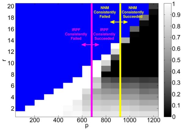
Mean relative reconstruction error using PF for various r values. The true rank is 8. Blue indicates untested cases (the number of degrees-of-freedom exceeded p). The success/failure regimes for NNM and IRPF are indicated with yellow and pink lines, respectively.

IV. Conclusion

This work investigated the IRPF algorithm as an alternative for NNM in the context of low-rank matrix recovery. IRPF is significantly faster than SDP-based NNM algorithms, and empirically has better recovery properties than NNM. While its theoretical properties are not yet fully established, IRPF has promising potential for practical matrix-recovery problems.

References

- [1].Recht B, Fazel M, Parrilo PA. Guaranteed Minimum Rank Solutions to Linear Matrix Equations Via Nuclear Norm Minimization preprint. 2008 [Online]. Available: http://arxiv.org/abs/0706.4138. [Google Scholar]
- [2].Candes E, Recht B. Exact Matrix Completion Via Convex Optimization preprint. 2008 [Online]. Available: http://arxiv.org/abs/0805.4471. [Google Scholar]
- [3].Recht B, Xu W, Hassibi B. Necessary and Sufficient Conditions for Success of the Nuclear Norm Heuristic for Rank Minimization preprint. 2008 [Online]. Available: http://arxiv.org/abs/0809.1260. [Google Scholar]
- [4].Fazel M, Hindi H, Boyd S. Proc. Amer. Control Conf. Arlington, VA: 2001. “A rank minimization heuristic with application to minimum order system approximation,”; pp. 4734–4739. [Google Scholar]
- [5].Fazel M, Hindi H, Boyd S. Proc. Amer. Control Conf. Denver, CO: 2003. “Log-det heuristic for matrix rank minimization with applications to Hankel and Euclidean distance matrices,”; pp. 2156–2162. [Google Scholar]
- [6].Grigoriadis K, Beran E. “Alternating projection algorithms for linear matrix inequalities problems with rank constraints,”. In: Ghaoui LE, Niculescu S-I, editors. Advances in Linear Matrix Inequality Methods in Control. SIAM; Philadelphia, PA: 2000. pp. 251–267. [Google Scholar]
- [7].Candes E, Romberg J, Tao T. “Robust uncertainty principles: Exact signal reconstruction from highly incomplete frequency information,”. IEEE Trans. Inform. Theory. 2006 Feb;52(2):489–509. [Google Scholar]
- [8].Donoho D. “Compressed sensing,”. IEEE Trans Inform. Theory. 2006 Apr;52(4):1289–1306. [Google Scholar]
- [9].Toh KC, Todd MJ, Tütüncü RH. SDPT3—A MATLAB Software Package for Semidefinite-Quadratic-Linear Programming. [Online]. Available: http://www.math.nus.edu.sg/mattohkc/sdpt3.html. [Google Scholar]
- [10].Sturm JF. “Using SeDuMi 1.02, a MATLAB toolbox for optimization over symmetric cones,”. Optim. Meth. Softw. 1999;11-12:625–653. [Google Scholar]
- [11].Rennie JDM, Srebro N. Proc. ICML. 2005. “Fast maximum margin matrix factorization for collaborative prediction,”. [Google Scholar]
- [12].Cai J-F, Candes E, Shen Z. A Singular Value Thresholding Algorithm for Matrix Completion preprint. 2008 [Online]. Available: http://arxiv.org/abs/0810.3286. [Google Scholar]
- [13].Vidal R, Tron R, Hartley R. “Multiframe motion segmentation with missing data using PowerFactorization and GPCA,”. Int. J. Comput. Vis. 2008;79:85–105. [Google Scholar]
- [14].Golub G, van Loan C. Matrix Computations. 3rd ed The Johns Hopkins Univ. Press; Baltimore, MD: 1996. [Google Scholar]