Linkage Analysis without Defined Pedigrees

Abstract

The need to collect accurate and complete pedigree information has been a drawback of family-based linkage and association studies. Even in case-control studies, investigators should be aware of, and condition on, familial relationships. In SNP genome scans, relatedness can be directly inferred from the genetic data rather than determined through interviews. Various methods of estimating relatedness have previously been implemented, most notably in PLINK. We present new fast and accurate algorithms for estimating global and local kinship coefficients from dense SNP genotypes. These algorithms require only a single pass through the SNP genotype data. We also show that these estimates can be used to cluster individuals into pedigrees. With these estimates in hand, QTL linkage analysis proceeds via traditional variance components methods without any prior relationship information. We demonstrate the success of our algorithms on simulated and real data sets. Our procedures make linkage analysis as easy as a typical genomewide association study.

Introduction

Family relationships lie at the heart of all gene mapping studies. Pedigree structure determines the expected amount of genetic sharing in linkage studies and accounts for background polygenic similarities in association studies. Even case-control studies need to be aware of familial relationships to avoid violating the assumption of independent subjects. There are a number of ways to measure relatedness, but the best rely on the number of alleles that a pair of individuals share identical by descent (IBD) at a random locus. Two sampled alleles at the same locus are identical by descent if they are both inherited copies of the same ancestral allele. This differs from identity by state (IBS), where the two sampled alleles simply have the same value. Depending on study design and the nature of measured phenotypes, IBD plays a direct or an indirect role in all family-based association and linkage studies. In quantitative trait locus (QTL) mapping, kinship coefficients are fundamental. Misspecfication of the degree of relatedness in a sample can dramatically affect results, in some cases reducing the power to detect a signal and in other cases leading to a false positive. It is therefore crucial to accurately determine IBD sharing among subjects before declaring linkage or association.

As the density of marker maps has increased, interest has grown in using genotypes to estimate relatedness. The early research of Thompson [Thompson, 1974, 1975] focused on identifying and quantifying pairwise relationships from genotype data. Her seminal contributions inspired the construction and implementation of several methods to test specific relationships in human pedigree analysis [Boehnke and Cox, 1997; Ehm and Wagner, 1998; Epstein et al., 2000; McPeek and Sun, 2000; Lange et al., 2001; Sun et al., 2002; Teo et al., 2009]. These methods, regardless of whether they are frequentist or Bayesian, benefit from prior knowledge of relationships. They excel at detecting relationship misspecifications. Relationship assignment is more difficult, particularly in population surveys omitting family history and in population isolates where pedigree boundaries are obscure and inbreeding may result in complex relationships [Queller and Goodnight, 1989; Mousseau et al., 1998; Lynch and Ritland, 1999; Wang, 2002].

The strategy of applying genotype-based estimated IBD rates to improve relationship information in gene mapping algorithms has been used to good effect for several years. In studies of non-human populations, QTL analysis is most common and thus the use of IBD and kinship estimates has received considerable attention [Slate et al., 2002; Slate, 2005]. In human studies, these estimates were found early on to be useful to map recessive traits in sibships [Leutenegger et al., 2002, 2003]. More recently, research has continued briskly to examine IBD estimation in extended pedigree and denser marker sets [Nelson et al., 2006; Purcell et al., 2007; Anderson and Weir, 2007; Albers et al., 2008; Thompson, 2008].

Genome-wide association studies (GWAS) with case-control samples [Risch and Merikangas, 1996] can be compromised by several complications. Well conceived studies always correct for genotyping success rates and ethnic stratification [Pritchard and Rosenberg, 1999; Reich and Goldstein, 2001; Satten et al., 2001]. It is also important to eliminate or correct for cryptic relatedness. Failure to do so can be catastrophic [Voight and Pritchard, 2005]. This has lead to the development of association tests that condition on evidence of relatedness in the data [Devlin and Roeder, 1999; Bacanu et al., 2000; Slager and Schaid, 2001; Voight and Pritchard, 2005; Purcell et al., 2007] or on both relatedness and ethnic stratification simultaneously [Yu et al., 2006].

Kinship coefficients are the most useful summaries of pairwise IBD sharing; these come in two flavors, global (also known as theoretical and unconditional) and local (a.k.a. empirical and conditional). A global kinship coefficient between two relatives i and j is not tied to a specific locus or observed genotypes. It is defined as the probability that a randomly sampled allele from i at some anonymous locus is IBD to a randomly sampled allele from j at the same locus. If i and j coincide, then sampling is done with replacement. Given accurate and complete pedigree structures, global kinship coefficients are straightforward to compute [Lange, 2002]. The local kinship coefficient of i and j measures their relationship at a specific locus conditioned on all observed genotypes. The process of sampling and comparing alleles is the same in both settings, but the probabilities differ in being unconditional or conditional.

In this paper we describe three new, fast algorithms that exploit whole-genome data on single nucleotide polymorphisms (SNPs) to estimate kinship coefficients and find related individuals. These algorithms run very quickly, the rate limiting step is a single pass through the SNP genotype data. No prior knowledge of relatedness is invoked. The first algorithm estimates global kinship coefficients, the second estimates local kinship coefficients, and the third applies the global estimates to cluster individuals into pedigrees. We show that the results of the algorithms can be used to map quantitative trait loci, without the time and expense of determining accurate and complete pedigree structures.

The first algorithm we present relies on an exact method-of-moments formula extended to all markers [Milligan, 2003]. In estimating the global kinship coefficient between a pair of individuals, it assumes a homogeneous population with known allele frequencies. The algorithm is both fast and accurate. Accuracy is almost inevitable given the overwhelming number of SNPs currently being typed. The generated global kinship coefficients can quickly identify any misspecified or cryptic relatedness.

Various approaches to a method of moments analysis for IBD and kinship estimation have been previously investigated and implemented [Purcell et al., 2007; Browning, 2008; Browning and Browning, 2010], however most of these have used hidden Markov model (HMM) techniques, which may be computationally intensive. More recently, some maximum likelihood methods have also been proposed and implemented [Choi et al., 2009; Thornton and McPeek, 2010]. Another interesting implementation [Manichaikul et al., 2010] relaxes the assumption of a homogenous sample population, allowing subsets of the sample to have different allele frequencies.

The second algorithm we present applies dynamic programming to minimize an objective function capturing local IBD sharing. The objective function includes a penalty tying together the local method of moments estimates. In this fashion the weak marker-by-marker estimates borrow strength from one another. At any particular locus, for each two individuals, there are four possible pairs of alleles, where one allele is from each individual. The kinship state counts how many of these pairs of alleles are IBD. The algorithm requires just a single pass through the data to assign one of the four possible kinship states 0, 1, 2, or 4 at each marker to a pair of individuals. The fact that the algorithm imputes a discrete state rather than estimates a continuous coefficient improves accuracy and eliminates computationally expensive iteration. This accuracy and speed differentiates our algorithm from the previous approaches to kinship estimation.

The third algorithm we present clusters individuals into pedigrees using the global kinship estimates and a standard graph theory procedure that finds connected components within a graph. Since the individual algorithms are each fast, this hybrid procedure quickly generates clusters of related individuals.

We check the accuracy of the algorithms on simulated data and demonstrate on real data how they can be combined to map a QTL in the absence of firm pedigrees. These successful trials of the algorithms suggest that they will be of considerable utility in dense genome scans for linkage or association.

Methods

Algorithm 1: Global Kinship Coefficient Estimation

To estimate global kinship coefficients, we begin by writing the expected number of IBS matches between individuals u and v under random sampling as

$$e_{uv}=\sum _{i=1}^m\left[{\Phi }_{uv}+(1-{\Phi }_{uv})\left(p_i^2+q_i^2\right)\right],$$ (1)

where m is the number of SNPs, Φ_uv is the global kinship coefficient for u and v, p_i is the major allele frequency at SNP i, and q_i = 1 – p_i is the minor allele frequency. The first term in the summation accounts for matches that are IBD at i, while the second term accounts for matches that are IBS but not IBD. Equation (1) holds for both autosomal and X-linked SNPs. Solving for Φ_uv gives

$${\Phi }_{uv}=\frac{e_{uv}-\sum _{i=1}^m(p_i^2+q_i^2)}{m-\sum _{i=1}^m(p_i^2+q_i^2)}.$$ (2)

To derive our method of moments estimator, we equate e_uv to the observed number of IBS matches over all m SNPs. Because kinship coefficients involve random sampling of alleles, we interpret the observed number of IBS matches as a conditional expectation given the SNP genotypes of u and v. Thus, if i is an autosomal SNP, then we define the observed number of IBS matches at SNP i as

$$o_{uv}^i=\frac{1}{4}\left[1_{\{I_i=K_i\}}+1_{\{I_i+L_i\}}+1_{\{J_i=K_i\}}+1_{\{J_i=L_i\}}\right],$$

where I_i and J_i represent the alleles of u at SNP i, K_i and L_i represent the alleles of v at i, and 1 with a subscripted condition takes the value 1 when the condition is met and 0 otherwise. If SNP i is X-linked, then the same formula applies when u and v are both females. When u is male and v is female,

$$o_{uv}^i=\frac{1}{2}\left[1_{\{I_i=K_i\}}+1_{\{I_i=L_i\}}\right],$$

and when u and v are both males, $o_{uv}^i=1_{\{I_i=K_i\}}$. Computation of the observed number of matches between u and v requires a single pass through the genome. Substitution of ${\sum }_{i=1}^m{o}_{uv}^i$ for e_uv in equation (2) now yields our estimate of their global kinship coefficient.

Because formula (2) depends heavily on allele frequencies, it is a good idea to check its sensitivity to errors in these frequencies. Supplementary Tables 25-34 show the impact of various kinds of errors on estimated global kinship coefficients. The bottom line is that random errors are relatively harmless, but systematic errors significantly degrade global kinship coefficient estimates.

Algorithm 2: Local Kinship Coefficient Imputation

To estimate local kinship coefficients, we invoke formula (2) in a small window centered on the current SNP j. This gives the point estimate

$$y_j=\frac{{\sum }_{i=1}^w[o_{uv}^i-(p_i^2+q_i^2)]}{{\sum }_{i=1}^w[1-(p_i^2+q_i^2)]},$$

where w counts the number of SNPs in the window. In practice, we use windows that cover roughly 50 Kbp on either side of the current SNP. (If one suspects very large blocks of linkage disequilibrium in the population, one may use even larger windows.) The estimates y_j are very noisy. To improve matters, we substitute imputation for estimation. Given full information, one can easily decide how many alleles two relatives u and v share IBD at SNP j. The local kinship coefficient between them at SNP j therefore takes one of the four values 0, $\frac{1}{4}$, $\frac{1}{2}$, or 1. (We note that our kinship estimation procedures also work with inbred population, as evident by allowing the value 1 for a local kinship coefficient.) The goal now is to impute one of these four numbers at each SNP j. At SNP j call this number z_j.

Imputation of the state variables z_j is guided by several principles. First, z_j should resemble y_j on average. Second, z_j takes jumps at IBD block boundaries but is otherwise constant. Because IBD blocks tend to be long, these jumps should be rare. Third, one should use observed SNP genotypes to narrow the range of possible values of z_j.

Suppose we record the observed number $o_{uv}^j$ of IBS matches at each SNP j. The condition $o_{uv}^j=1$ is a necessary but not a sufficient condition for z_j = 1. More importantly, the condition $o_{uv}^j=0$ is a sufficient but not a necessary condition for z_j = 0. If we find two SNPs i and j less than 1 Mbp apart with $o_{uv}^i=o_{uv}^j=0$, then we assign all intervening SNPs k the state variable z_k = 0. This rule is quite successful at determining regions of no IBD sharing. An intervening SNP k with z_k ≠ 0 would constitute evidence of two recombination events in a 1 Mbp interval, a very unlikely scenario in most pedigrees.

These considerations motivate simultaneous fitting and smoothing. We proceed by minimizing the objective function

$$f(z_1,\dots ,z_m)=\sum _{i=1}^m{(y_i-z_i)}^2+{\lambda }_1\sum _{i=1}^m{(z_i-{\Phi }_{uv})}^2+{\lambda }_2\sum _{i=1}^{m-1}{(z_{i+1}-z_i)}^2$$ (3)

subject to the restrictions $z_i\in \{o,\frac{1}{4},\frac{1}{2},1\}$ and to our interval rule for assigning z_i = 0. Here λ₁ and λ₂ are nonnegative tuning constants and Φ_uv is the estimated global kinship coefficient for the pair. In practice, we work chromosome by chromosome, so Φ_uv is specific to the current chromosome and m is the number of SNPs on that chromosome. Readers familiar with the fused lasso [Tibshirani, 1996; Tibshirani et al., 2005] will recognize our debt to lasso penalized estimation in constructing the objective function f(z₁, … , z_m).

Fortunately, the z_i values that minimize this objective function can be found in a single pass through the data using standard dynamic programming techniques. Our solution begins by reformulating the objective function as

$$f(z_i,\dots ,z_m)=\sum _{i=1}^m{f}_i\left(z_i\right)+\sum _{i=1}^{m-1}{g}_i(z_i,z_{i+1}).$$

The loss function f_i(z_i) = (y_i–z_i)² + λ₁(z_i–Φ_uv)² has just four values. The penalty function g_i(z_i, z_i+1) = λ₂(z_i+1–z_i)². To find the optimal z_i values by dynamic programming, define the partial solutions h₁(z₁) = f₁(z₁) and

$$h_k\left(z_k\right)=\underset{z_{1,\dots ,}{z}_{k-1}}{\min }\left\{\sum _{i=1}^k{f}_i\left(z_i\right)+\sum _{i=1}^{k-1}{g}_i(z_i,z_{i+1})\right\}$$

for k > 1. If one records the values $h_k\left(0\right),h_k\left(\frac{1}{4}\right),h_k\left(\frac{1}{2}\right)$, and h_k(1), then the recurrence

$$h_k\left(z_k\right)=\underset{z_{k-1}}{\min }\{h_{k-1}\left(z_{k-1}\right)+g_{k-1}(z_{k-1},z_k)\}+f_k\left(z_k\right)$$

determines the next partial solution. Finally, z_m is the value that minimizes h_m(z_m). The standard traceback procedure supplies the rest of the solution z₁, … , z_m–1 once z_m is imputed.

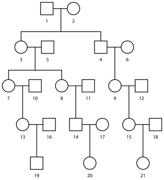
Our remaining task is to find the best penalty weights, λ₁ and λ₂ in equation (3) for various relative pairs. Equation (3) shows that λ₁ determines the extent of the penalty when the local kinship coefficient estimate diverges from the global estimate. Similarly, λ₂ determines the extent of the penalty when there are frequent changes in the local IBD status. To determine which penalty weights would work well, we used 100 simulated replicates of the pedigree in Figure 1, each typed at the same 200K SNPs. We searched for the penalty weights that minimized the average absolute difference between the estimated and true local kinship coefficients. Fortunately, there was a pair of values that minimized this difference for all tested relationships and both long and short chromosomes. Setting λ₁ = 0 and λ₂ = 100 gives a quick, accurate, and universal algorithm for estimating local kinship coefficients. The Supplementary Material describes the grid search performed and Supplementary Tables 35-38 show the results of our search for the best penalty weights.

Figure 1.

Structure of simulated pedigrees.

Algorithm 3: Construction of Pedigree Clusters

To cluster individuals into pedigrees we use the global kinship estimates and a standard graph theory procedure. In this hybrid algorithm, genotyped individuals constitute the nodes of an undirected graph. An edge is drawn between a pair of individuals if their estimated global kinship estimate exceeds a fixed cutoff value. A standard graph theory procedure [Aho and Hopcroft, 1974] then clusters the individuals into pedigrees by finding the connected components of the graph. This procedure operates by visiting successive nodes and merging existing components containing the current node.

With a high cutoff value, say 0.2, only close relationships will contribute to clustering. Thus, individuals with no close genotyped relatives form isolated one-person clusters. With a low cutoff, say 0.02, distant relatives are clustered even if their intervening close relatives are not genotyped.

Results

Global Kinship Coefficient Estimation

To determine the accuracy of the global kinship estimator, we simulated genotypes for 500 replicates of the pedigree depicted in Figure 1 at each of four SNP scan densities: 10K, 100K, 200K, and 500K SNPs per genome. For the sake of simplicity, we took genetic map distances proportional to physical distances and independent of sex. We used the Caucasian allele frequencies published by Affymetrix for their commercial SNP arrays. Simulation by gene dropping allowed us to record IBD status at each and every SNP. Of course, all estimates were calculated without reference to this knowledge. To assess accuracy, we estimated global kinship coefficients for eight relative pairs in the pedigree. For the sake of brevity, we discuss here the results for two pairs. All our results can be found in Supplementary Supplementary Tables 1-24.

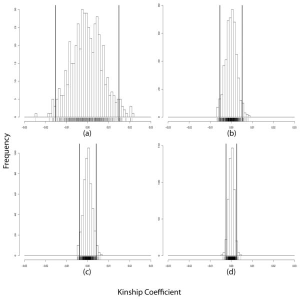
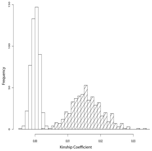
Consider first the pair of unrelated individuals 1 and 2, both founders of the pedigree (Figure 1). We computed the minimum, mean, maximum and standard deviation of the estimates for this pair over the 500 replicates at each of the four SNP densities (see Supplementary Table 1). The mean value for each density is essentially zero, confirming lack of bias in unrelateds. To formally test for bias, we conducted a Kolmogorov-Smirnov (KS) test comparing the empiric distribution against a normal distribution with mean 0 and standard deviation taken from the estimates. The KS test was unable to reject the null hypothesis of unbiasedness (see Supplementary Table 3). Figure 2 shows histograms of the estimates for this pair for the 10K, 100K, 200K, and 500K densities. Not surprisingly, the standard deviations of the estimates shrink and accuracy improves as the density of SNPs increases. At the 500K SNP density, it possible to distinguish the degree of relatedness of the unrelated pair 1 and 2 from that of the distantly related pair of cousins 7 and 21 in the pedigree. Figure 3 displays the two histograms side by side. The difference between the kinship coefficient (0.0) of the pair 1 and 2 and the kinship coefficient (0.015625) of the cousins 7 and 21 is probably near the lower bound of what is detectable. From our perspective, this level of resolution is more than adequate for practical purposes.

Figure 2.

Global kinship coefficient estimates for the unrelated pair 1 and 2 (true global kinship coefficient 0.0) using: (a) 10K SNPs, (b) 100K SNPs, (c) 200K SNPs, and (d) 500K SNPs. The left and right bold vertical lines represent ±2 standard deviations.

Figure 3.

Distributions of global kinship coefficient estimates using 500K SNPs for unrelated pair 1 and 2 (unshaded, true global kinship coefficient 0.0) versus distantly related pair 7 and 21 (shaded, first cousins twice removed, true global kinship coefficient 0.015625).

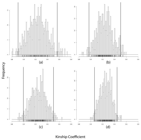
Second degree relatives such as the uncle-niece pair 4 and 7 in Figure 1 have a global kinship coefficient of 0.125. The mean value of our global kinship estimator accurately captures this level of relatedness at all four SNP densities (see Supplementary Table 7). Again, better mean estimates and smaller standard deviations are seen with increasing numbers of SNPs (Figure 4). As before, the KS test does not reject the hypothesis of unbiasedness (see Supplementary Table 9). With 500K SNPs there is a good separation between the distributions of the estimators for all relative pairs with global kinship coefficients in excess of 0.007 (Supplementary Figures 1-5). Of course, one cannot distinguish pairs with the same global kinship coefficients. Examples include siblings versus parent-offspring and uncle-niece versus grandparent-grandchild. Other more detailed coefficients of relatedness help in making these distinctions, but estimation of these detailed identity coefficients is more difficult.

Figure 4.

Global kinship coefficient estimates for uncle-niece pair 4 and 7 (true global kinship coefficient 0.125) using: (a) 10K SNPs, (b) 100K SNPs, (c) 200K SNPs, and (d) 500K SNPs. The left and right bold vertical lines represent ±2 standard deviations.

The software package PLINK currently has the most widely used method for estimating global relatedness from genome-wide SNP data [Purcell et al., 2007]. PLINK employs a method-of-moments algorithm that estimates IBD sharing and is more complicated than the method-of-moments algorithm described here. We analyzed the same set of 500 simulated pedigrees detailed above using PLINK’s genome option, again without reference to the known relationships. Supplementary Tables 2, 5, 8, 11, 14, 17, 20 and 23 show the comparisons between our estimates and PLINK’s estimates. These tables illustrate that our simpler method-of-moments algorithm performs as well as PLINK in all instances, and slightly better as the individuals become more distantly related.

We also tested our global kinship algorithm on a real data set from the San Antonio Family Heart Study (SAFHS) [Mitchell et al., 1996]. The data set consists of 1942 immigrants, or descendents of immigrants, from near Monterrey, Mexico who have settled in San Antonio in the US. We restricted our analysis to the 858 individuals genotyped on the Illumina 550K SNP platform. In the reported pedigrees, 51 people in this subset are unrelated to the remaining 807, who were spread over 45 pedigrees ranging in size from 3 to 62 people. Allele frequencies for the SNP markers typed in this study were previously summarized [Göring et al., 2007].

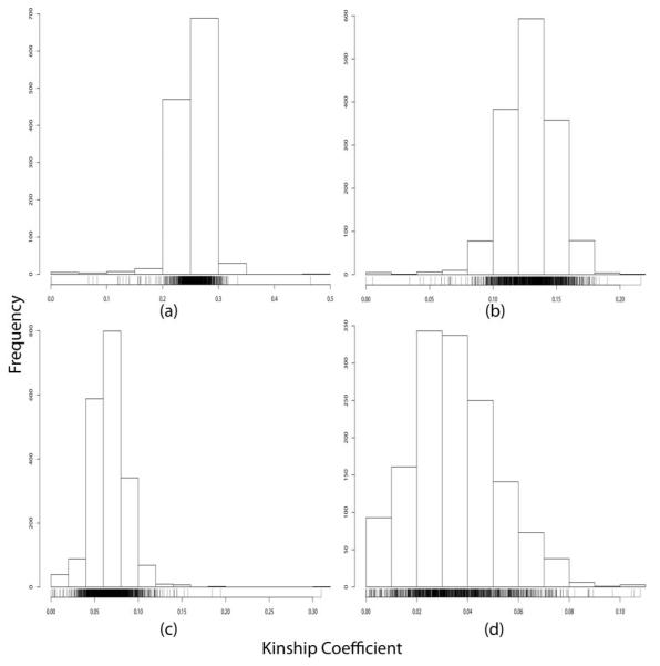
We considered all pairs of individuals in the data with global kinship coefficients of 0.25, 0.125, 0.0625, and 0.03125 based on their self-reported ancestry. For each pair we estimated a global kinship coefficient via our algorithm. Figure 5 and Table 1 show the results. The estimates appear accurate and unbiased. To assess the sensitivity of these conclusions to misspecified allele frequencies, we conducted extensive simulation studies. When major allele frequencies are systematically underestimated, global kinship coefficients are overestimated. The reverse occurs when major allele frequencies are systematically overestimated. These biases are a natural consequence of equation (2) in the Methods section. Allele frequency misspecification does not appear to have much impact on the variances of the estimates. Details of this analysis for an uncle-niece pair is given in Supplementary Tables 25-34. Fortunately, the large number of published GWAS studies ensures accurate allele frequencies for most major populations.

Figure 5.

SNP-based global kinship coefficient estimates for SAFHS pairs with pedigree-based global kinship coefficient of: (a) 0.25, (b) 0.125, (c) 0.0625, and (d) 0.03125.

Table 1.

Global kinship coefficient estimates for selected pairs of individuals from the SAFHS data set.

Pedigree-based Global Kinship	Number of Pairs	SNP-based Global Kinship, Mean (Standard Deviation)
0.25	1218	0.2533 (0.030)
0.125	1521	0.1291 (0.021)
0.0625	1950	0.0667 (0.021)
0.03125	1454	0.0349 (0.017)

Local Kinship Coefficient Imputation

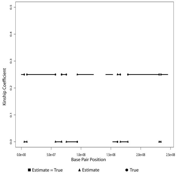
In our local kinship estimation algorithm, the strength of the penalty depends on two tuning constants. We found that one of these could be set to 0 and the other to a single positive value appropriate to all SNPs and relative pairs. (See the Methods section and Supplementary Tables 35-38). These universal choices simplify the already fast dynamic programming algorithm. For each SNP density, we used the previously described 500 simulated replicates of the pedigree depicted in Figure 1 to assess the accuracy of the local kinship estimates. Figure 6 plots the local kinship coefficient estimate along chromosome 1 for a typical replicate of an uncle-niece pair. For this replicate only 249 of the 40,326 SNPs on chromosome 1, roughly 0.6%, were assigned an incorrect kinship state. This replicate is typical in the sense that it gives the median error rate across all SNPs on chromosome 1. Supplementary Figure 30 shows the distribution of the error rates over all replicates. Comparisons of estimated and true local kinship coefficients for other relationships and SNP densities appear in Supplementary Figures 7-13 and Supplementary Tables 39-46.

Figure 6.

True and estimated local kinship coefficients on chromosome 1 for a typical replicate of the 500K SNP set using the uncle-niece pair 4 and 7 (true global kinship coefficient 0.125). Each SNP’s local kinship coefficient is shown with a small square when the true and estimated values are identical. When they differ, the true value is shown as a circle and the estimated as a triangle. Of the 40,326 SNPs depicted, 249 were assigned incorrect local kinship coefficients.

Overall, our results validate the accuracy of the local kinship algorithm. We obtained accurate results for all relative pairs examined and for all chromosomes, regardless of their length. Incorrect imputations occur at IBD block boundaries. Errors tend to extend one block at the expense of a neighboring block.

Construction of Pedigree Clusters

Our third goal was to cluster related individuals into groups using only estimated global kinship coefficients. These clusters, although lacking fully defined relationships, can replace standard pedigrees in QTL mapping. Recall that QTL mapping uses local kinship coefficients to locate the major gene determining trait variation. To account for background polygenic inheritance, it uses global kinship coefficients. More nuanced pedigree information is ignored.

We again used the simulated replicates of the pedigree in Figure 1 for testing. We ran the clustering algorithm ignoring the genotypes of individuals 7 through 12 at the cutoffs 0.2, 0.125, and 0.1. In all replicates, the remaining typed individuals cluster as expected (Supplementary Table 47).

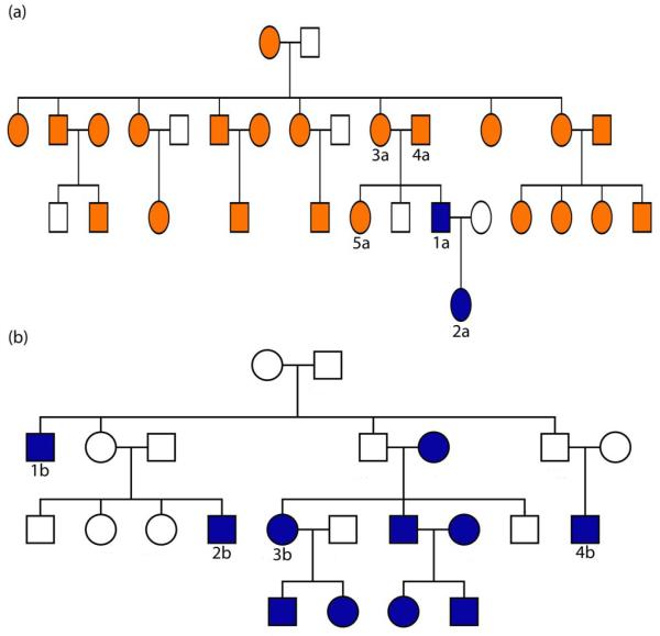
We also tested the clustering algorithm on the SAFHS data set. The pedigrees in the SAFHS data set are based on interviews and standard relationship testing procedures using the PREST software [Sun et al., 2002]. This type of software helps identify clear relationship misspecifications, but correct relationship reconstruction is harder to achieve, especially when inbreeding is present. After computing global kinship estimates, we clustered 858 individuals in the SAFHS data set with cutoffs of 0.2, 0.1, and 0.0625. Using a 0.2 cutoff, we clustered 740 of the individuals into 122 pedigrees of size 2 to 36. Figure 7 is an example of how our clusters compare to the pedigrees defined in the SAFHS data set. In this figure, individual 1a moves from pedigree (a) to pedigree (b) because he has estimated global kinship coefficients of 0.329, 0.201, 0.215, and 0.326 with individuals 1b, 2b, 3b, and 4b, respectively. After lowering the cutoff to 0.1, the two separate pedigrees merged because individual 1a has estimated global kinship coefficients of 0.193, 0.190, and 0.175 with individuals 3a, 4a, and 5a, respectively. Using a 0.1 cutoff, a total of 793 individuals were clustered into 31 pedigrees of size 2 to 568. Finally, using a cutoff of 0.0625, all 858 individuals were clustered into a single pedigree. Since all of the individuals claim ancestry from the same narrow region of Mexico, we believe our results reveal relationships not evident in the interviews.

Figure 7.

Example of cluster analysis results for the SAFHS data set. Two SAFHS pedigrees are shown: (a) and (b). Only individuals drawn in color had SNP genotypes. In the cluster analysis using a 0.2 cutoff, individual 1a and 2a cluster with pedigree (b), not with the other individuals in pedigree (a). Using a 0.1 cutoff, all individuals drawn in color cluster together in one pedigree. See the text for selected global kinship coefficient estimates.

QTL Analysis

Standard QTL mapping is based on a variance components model that represents QTL contributions as random effects [Hopper and Mathews, 1982; Almasy and Blangero, 1998; Lange, 2002]. The pertinent input include trait values, marker genotypes, and pedigree structures. Pedigree structures determine global kinship coefficients. Observed marker genotypes and pedigree structures jointly generate local kinship coefficients. Once the global and local kinship coefficients are computed, marker genotypes and pedigree structures can be discarded. As seen above, dense SNP genotyping allows one to circumvent pedigree structures altogether. Restricting the size of pedigrees avoids computational bottlenecks such as the inversion and storage of large matrices. Thus, it is a good idea to cluster individuals into pedigrees even though lumping them all into a single large pedigree is in principle consistent with gene mapping.

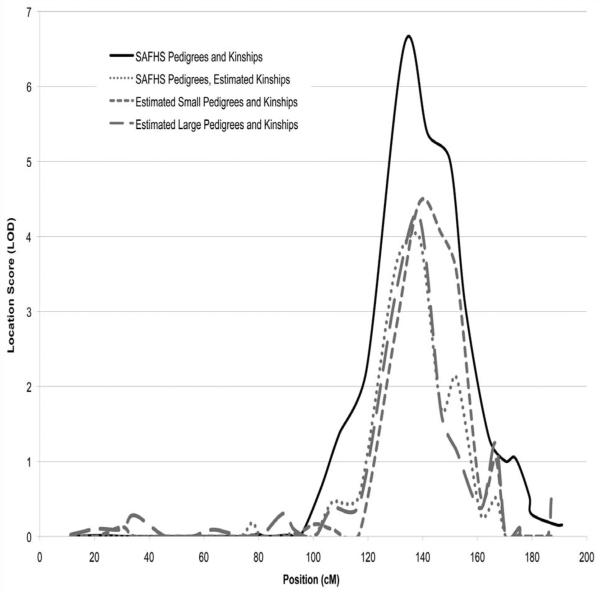
To test our kinship estimation algorithms in QTL mapping, we re-analyzed the SAFHS data set. This data set includes vannin 1 (VNN1) expression levels as a quantitative phenotype. Using microsatellite markers genotyped on roughly 1318 of the individuals, an eQTL for VNN1 was mapped near marker D6S1040 on chromosome 6 [Göring et al., 2007]. We sought to replicate this finding using only the dense SNP genotypes on 858 individuals, ignoring prior relationship information. We first performed traditional QTL linkage analysis on the SAFHS pedigrees and microsatellite genotypes, but restricted to the 858 individuals with SNP genotypes. The maximum LOD score was 6.5 at D6S1040. This is the same locus previously mapped in the entire data set with a higher LOD score [Göring et al., 2007]. We used the same variance components software with pedigrees as originally defined by the SAFHS study, but all local kinship coefficients estimated from the dense SNP genotypes. The maximum LOD score obtained was 4.2 at the SNP closest to the peak microsatellite marker. We next ran our standard variance components software ignoring reported pedigrees and relying on global and local kinship coefficients estimated from the dense SNP genotypes. In clustering individuals, we first used a global kinship cutoff of 0.2, a lax criterion that clusters based only on closely related individuals. The maximum LOD score obtained in this re-analysis was 4.5, at the same peak SNP. Finally, we performed the same analysis using a global kinship cutoff of 0.1 in our pedigree clustering, which allows clustering based on more distant relationships. Here the maximum LOD score was 4.3, again at the same peak SNP. LOD score curves for all four analyses are shown in Figure 8.

Figure 8.

QTL analyses of a subset of the SAFHS data set. The solid curve summarizes results using the SAFHS supplied pedigrees and microsatellite data. The short-dash curve summarizes results using the SAFHS pedigrees, but local kinship coefficients estimated from the SNP genotypes. The medium-dash curve summarizes results using reconstructed pedigrees with a 0.2 global kinship cutoff and global and local kinship coefficients estimated from SNP genotypes. The long-dash curve summarizes results using reconstructed pedigrees with a 0.1 global kinship cutoff and global and local kinship coefficients estimated from SNP genotypes.

The most time-consuming step in a variance component analysis is inverting an n × n matrix, where n is the size of the largest pedigree. Inversion takes on the order of n³ operations. Thus it is not surprising that the change from a largest pedigree of 36 individuals to one of 568 individuals, in practice means a run time increase from 20 seconds to 2.5 hours.

The drop in LOD scores from the original microsatellite data can be attributed to three possible reasons: (a) loss of information in reassembling the pedigrees, (b) poor values for the global kinship coefficients, and (c) poor values for the local kinship coefficients. Our simulations imply that these algorithms are finding excellent estimates for global kinship coefficients, so we rule out explanation (b). Some loss in power is to be expected when losing information on the specific relationships between each pair of individuals, which usually informs the kinship coefficient calculations. To compensate, refinements may well be possible in the pedigree clustering and local kinship imputation. However, the LOD scores that we obtain without pedigree information are still highly significant.

Discussion

In the past few years genome-wide association studies (GWAS) have scored some huge success in mapping genes influencing complex traits [Hindorff et al., 2009]. One enticement of case-control studies is their avoidance of the long and arduous task of collecting accurate and complete pedigree structures, particularly for the large pedigrees that contain the majority of linkage information. Despite the successes in the numerous GWAS studies undertaken, most of the variation of the complex traits investigated remains unexplained [Altshuler and Daly, 2007]. Undoubtedly some of the missing genetic effects are rare mutations. These will often remain hidden to association tests but may be exposed by well-designed linkage studies.

We propose an easier route to linkage analysis, one that does not require collecting pedigree structures. For a QTL, it should suffice to collect dense SNP genotyping of cases, and perhaps their first degree relatives, from regions of low demographic mobility. Alternatively, as in the SAFHS, one can sample immigrants from such a region. The algorithms we have presented can then quickly and accurately estimate all kinship coefficients and assemble pedigree clusters. Current variance components software, though designed to take in whole pedigrees, can easily be rewritten to substitute estimated coefficients in mapping genes influencing quantitative traits. For qualitative traits, we suggest also collecting the first degree relatives of the affecteds and recoding affecteds as 1 and unaffecteds as 0. Recoding turns a qualitative trait into a quantitative trait and renders it amenable to QTL mapping. Because asymptotic p-values are based on a multivariate normal distribution of trait values, nominal p-values would no longer be trustworthy, but they could still serve to quantify the evidence in favor of linkage. Ranking of markers is an indispensable guide in mounting further studies.

When presented with dense SNP data for linkage analysis, many geneticists currently use only a fraction of the data, roughly mimicking the density of a genome-wide microsatellite marker panel. This procedure wastes data and gives poor estimates of local kinship coefficients. Our procedures use all available data and work well with as few as 10K SNPs, particularly in estimating global kinship coefficients. Of course the methods we present do have some drawbacks as well. For example, there is no measure of uncertainty in the kinship coefficient results. Typically linkage analysis requires many fewer individuals than GWAS to reach genome-wide significance, greatly reducing the cost of gene mapping. Of course the linkage analysis may highlight a relatively broad genomic region, but still narrow enough to allow targeted sequencing in a follow-up study. One should keep in mind that marker based estimation of kinship coefficients also has something to offer in association testing. Here the primary benefit is control for background polygenic inheritance.

In closing let us emphasize one point. The shift to GWAS has found many common variants of ancient origin that would have been be hard to pinpoint through linkage studies. As a complementary tool, linkage can find rare variants of recent vintage that association studies cannot. With the procedures we outline, once a suitable population is found, linkage studies can be made as simple as GWAS.

References

- Aho AV, Hopcroft JE. The Design and Analysis of Computer Algorithms. Addison-Wesley Longman Publishing; Boston, MA: 1974. [Google Scholar]
- Albers CA, Stankovich J, Thomson R, Bahlo M, Kappen HJ. Multipoint approximations of identity-by-descent probabilities for accurate linkage analysis of distantly related individuals. Am J Hum Genet. 2008;82:607–622. doi: 10.1016/j.ajhg.2007.12.016. [DOI] [PMC free article] [PubMed] [Google Scholar]
- Almasy L, Blangero J. Multipoint quantitative-trait linkage analysis in general pedigrees. Am J Hum Genet. 1998;62:1198–1211. doi: 10.1086/301844. [DOI] [PMC free article] [PubMed] [Google Scholar]
- Altshuler D, Daly MJ. Guilt beyond a reasonable doubt. Nat Genet. 2007;39:813–815. doi: 10.1038/ng0707-813. [DOI] [PubMed] [Google Scholar]
- Anderson AD, Weir BS. A maximum-likelihood method for the estimation of pairwise relatedness in structured populations. Genetics. 2007;176:421–440. doi: 10.1534/genetics.106.063149. [DOI] [PMC free article] [PubMed] [Google Scholar]
- Bacanu SA, Devlin B, Roeder K. The power of genomic control. Am J Hum Genet. 2000;66:1933–1944. doi: 10.1086/302929. [DOI] [PMC free article] [PubMed] [Google Scholar]
- Boehnke M, Cox NJ. Accurate inference of relationships in sib-pair linkage studies. Am J Hum Genet. 1997;61:423–429. doi: 10.1086/514862. [DOI] [PMC free article] [PubMed] [Google Scholar]
- Browning SR. Estimation of pairwise identity by descent from dense genetic marker data in a population estimation of pairwise identity by descent from dense genetic marker data in a population sample of haplotypes. Genetics. 2008;178:2123–2132. doi: 10.1534/genetics.107.084624. [DOI] [PMC free article] [PubMed] [Google Scholar]
- Browning SR, Browning BL. High-resolution detection of identity by descent in unrelated individuals. Am J Hum Genet. 2010;86:526–539. doi: 10.1016/j.ajhg.2010.02.021. [DOI] [PMC free article] [PubMed] [Google Scholar]
- Choi Y, Wijsman EM, Weir BS. Case-control association testing in the presence of unknown relationships. Genet Epidemiol. 2009;33:668–678. doi: 10.1002/gepi.20418. [DOI] [PMC free article] [PubMed] [Google Scholar]
- Devlin B, Roeder K. Genomic control for association studies. Biometics. 1999;55:997–1004. doi: 10.1111/j.0006-341x.1999.00997.x. [DOI] [PubMed] [Google Scholar]
- Ehm MG, Wagner M. A test statistic to detect error in sib-pair relationships. Am J Hum Genet. 1998;62:181–188. doi: 10.1086/301668. [DOI] [PMC free article] [PubMed] [Google Scholar]
- Epstein MP, Duren WL, Boehnke M. Improved inference of relationship for pairs of individuals. Am J Hum Genet. 2000;67:1219–1231. doi: 10.1016/s0002-9297(07)62952-8. [DOI] [PMC free article] [PubMed] [Google Scholar]
- Göring HH, Curran JE, Johnson MP, Dyer TD, Charlesworth J, Cole SA, Jowett JB, Abraham LJ, Rainwater DL, Comuzzie AG, Mahaney MC, Almasy L, MacCluer JW, Kissebah AH, Collier GR, Moses EK, Blangero J. Discovery of expression QTLs using largescale transcriptional profiling in human lymphocytes. Nat Genet. 2007;39:1208–1216. doi: 10.1038/ng2119. [DOI] [PubMed] [Google Scholar]
- Hindorff LA, Junkins HA, Mehta JP, Manolio TA. [Accessed 1 April 2009];A catalog of published genome-wide association studies. 2009 Available at www.genome.gov/26525384.
- Hopper JL, Mathews JD. Extensions to multivariate normal models for pedigree analysis. Ann Hum Genet. 1982;46:373–383. doi: 10.1111/j.1469-1809.1982.tb01588.x. [DOI] [PubMed] [Google Scholar]
- Lange K. Mathematical and Statistical Methods for Genetic Analysis. 2nd edition Springer-Verlag; New York: 2002. [Google Scholar]
- Lange K, Cantor R, Horvath S, Perola M, Sabatti C, Sinsheimer J, Sobel E. Mendel version 4.0: A complete package for the exact genetic analysis of discrete traits in pedigree and population data sets. Am J Hum Genet. 2001;69(Suppl):504. [Google Scholar]
- Leutenegger AL, Génin E, Thompson EA, Clerget-Darpoux F. Impact of parental relationships in maximum lod score affected sib-pair method. Genet Epidemiol. 2002;23:413–425. doi: 10.1002/gepi.10190. [DOI] [PubMed] [Google Scholar]
- Leutenegger AL, Prum B, Génin E, Verny C, Lemainque A, Clerget-Darpoux F, Thompson EA. Estimation of the inbreeding coefficient through use of genomic data. Am J Hum Genet. 2003;73:516–523. doi: 10.1086/378207. [DOI] [PMC free article] [PubMed] [Google Scholar]
- Lynch M, Ritland K. Estimation of pairwise relatedness with molecular markers. Genetics. 1999;152:1753–1766. doi: 10.1093/genetics/152.4.1753. [DOI] [PMC free article] [PubMed] [Google Scholar]
- Manichaikul A, Mychaleckyj JC, Rich SS, Daly K, Sale M, Chen WM. Robust relationship inference in genome-wide association studies. Bioinformatics. 2010;26:2867–2873. doi: 10.1093/bioinformatics/btq559. [DOI] [PMC free article] [PubMed] [Google Scholar]
- McPeek MS, Sun L. Statistical tests for detection of misspecified relationships by use of genome-screen data. Am J Hum Genet. 2000;66:1076–1094. doi: 10.1086/302800. [DOI] [PMC free article] [PubMed] [Google Scholar]
- Milligan BG. Maximum-likelihood estimation of relatedness. Genetics. 2003;163:1153–1167. doi: 10.1093/genetics/163.3.1153. [DOI] [PMC free article] [PubMed] [Google Scholar]
- Mitchell BD, Kammerer CM, Blangero J, Mahaney MC, Rainwater DL, Dyke B, Hixson JE, Henkel RD, Sharp RM, Comuzzie AG, VandeBerg JL, Stern MP, W MJ. Genetic and environmental contributions to cardiovascular risk factors in mexican americans. The San Antonio Family Heart Study. Circulation. 1996;94:2159–2170. doi: 10.1161/01.cir.94.9.2159. [DOI] [PubMed] [Google Scholar]
- Mousseau TA, Ritland K, Heath DD. A novel method for estimating heritability using molecular markers. Heredity. 1998;80:218–224. [Google Scholar]
- Nelson SF, Merriman B, Chen Z, Ogdie M, Stone J, Strom S. Applications of pedigree-free identity-by-descent mapping to localizing disease genes. Am J Hum Genet. 2006;79(Suppl) Abstract 1530. [Google Scholar]
- Pritchard JK, Rosenberg NA. Use of unlinked genetic markers to detect population stratification in association studies. Am J Hum Genet. 1999;65:220–228. doi: 10.1086/302449. [DOI] [PMC free article] [PubMed] [Google Scholar]
- Purcell S, Neale B, Todd-Brown K, Thomas L, Ferreira MAR, Bender D, Maller J, Sklar P, de Bakker PIW, Daly MJ, Sham PC. Plink: a toolset for whole-genome association and population-based linkage analysis. Am J Hum Genet. 2007;81:559–575. doi: 10.1086/519795. [DOI] [PMC free article] [PubMed] [Google Scholar]
- Queller DC, Goodnight KF. Estimating relatedness using genetic markers. Evolution. 1989;43:258–275. doi: 10.1111/j.1558-5646.1989.tb04226.x. [DOI] [PubMed] [Google Scholar]
- Reich D, Goldstein D. Detecting association in a case-control study while correcting for population stratification. Genet Epidemiol. 2001;20:4–16. doi: 10.1002/1098-2272(200101)20:1<4::AID-GEPI2>3.0.CO;2-T. [DOI] [PubMed] [Google Scholar]
- Risch N, Merikangas K. The future of genetic studies of complex human diseases. Science. 1996;273:1516–1517. doi: 10.1126/science.273.5281.1516. [DOI] [PubMed] [Google Scholar]
- Satten GA, Flanders WD, Yang Q. Accounting for unmeasured population substructure in case-control studies of genetic association using a novel latent-class model. Am J Hum Genet. 2001;68:466–477. doi: 10.1086/318195. [DOI] [PMC free article] [PubMed] [Google Scholar]
- Slager SL, Schaid DJ. Evaluation of candidate genes in case-control studies: A statistical method to account for related subjects. Am J Hum Genet. 2001;68:1457–1462. doi: 10.1086/320608. [DOI] [PMC free article] [PubMed] [Google Scholar]
- Slate J. Quantitative trait locus mapping in natural populations: progress, caveats and future directions. Mol Ecology. 2005;14:363–379. doi: 10.1111/j.1365-294X.2004.02378.x. [DOI] [PubMed] [Google Scholar]
- Slate J, Visscher PM, MacGregor S, Stevens D, Tate ML, Pemberton JM. A genome scan for quantitative trait loci in a wild population of red deer (cervus elaphus) Genetics. 2002;162:1863–1873. doi: 10.1093/genetics/162.4.1863. [DOI] [PMC free article] [PubMed] [Google Scholar]
- Sun L, Wilder K, McPeek MS. Enhanced pedigree error detection. Hum Hered. 2002;54:99–110. doi: 10.1159/000067666. [DOI] [PubMed] [Google Scholar]
- Teo YY, Fry AE, Sanjoaquin MA, Pederson B, Small K, Rockett KA, Kwiatkowski DP, Clark TG. Assessing genuine parents-offspring trios for genetic association studies. Hum Hered. 2009;67:26–37. doi: 10.1159/000164396. [DOI] [PMC free article] [PubMed] [Google Scholar]
- Thompson E. The estimation of pairwise relationships. Ann Hum Genet. 1975;39:173–188. doi: 10.1111/j.1469-1809.1975.tb00120.x. [DOI] [PubMed] [Google Scholar]
- Thompson EA. Gene identities and multiple relationships. Biometrics. 1974;30:667–680. [PubMed] [Google Scholar]
- Thompson EA. The ibd process along four chromosomes. Theoret Pop Bio. 2008;73:369–373. doi: 10.1016/j.tpb.2007.11.011. [DOI] [PMC free article] [PubMed] [Google Scholar]
- Thornton T, McPeek MS. Roadtrips: case-control association testing with partially or completely unknown population and pedigree structure. Am J Hum Genet. 2010;86:172–184. doi: 10.1016/j.ajhg.2010.01.001. [DOI] [PMC free article] [PubMed] [Google Scholar]
- Tibshirani R. Regression shrinkage and selection via the lasso. J R Stat Soc Ser B. 1996;58:267–288. [Google Scholar]
- Tibshirani R, Saunders M, Rosset S, Zhu J, Knight K. Sparsity and smoothness via the fused lasso. J R Stat Soc Ser B. 2005;67:91–108. [Google Scholar]
- Voight BF, Pritchard JK. Confounding from cryptic relatedness in case-control association studies. PLoS Genet. 2005;1:e32. doi: 10.1371/journal.pgen.0010032. [DOI] [PMC free article] [PubMed] [Google Scholar]
- Wang J. An estimator for pairwise relatedness using molecular markers. Genetics. 2002;160:1203–1215. doi: 10.1093/genetics/160.3.1203. [DOI] [PMC free article] [PubMed] [Google Scholar]
- Yu J, Pressoir G, Briggs WH, Vroh Bi I, Yamasaki M, Doebley JF, McMullen MD, Gaut BS, Nielsen DM, Holland JB, Kresovich S, Buckler ES. A unified mixed-model method for association mapping that accounts for multiple levels of relatedness. Nat Genet. 2006;38:203–208. doi: 10.1038/ng1702. [DOI] [PubMed] [Google Scholar]
Associated Data
This section collects any data citations, data availability statements, or supplementary materials included in this article.