

Abstract
DNA arrays have been widely used to perform transcriptome-wide analysis of gene expression, and many methods have been developed to measure gene expression variability and to compare gene expression between conditions. Because RNA-seq is also becoming increasingly popular for transcriptome characterization, the possibility exists for further quantification of individual alternative transcript isoforms, and therefore for estimating the relative ratios of alternative splice forms within a given gene. Changes in splicing ratios, even without changes in overall gene expression, may have important phenotypic effects. Here we have developed statistical methodology to measure variability in splicing ratios within conditions, to compare it between conditions, and to identify genes with condition-specific splicing ratios. Furthermore, we have developed methodology to deconvolute the relative contribution of variability in gene expression versus variability in splicing ratios to the overall variability of transcript abundances. As a proof of concept, we have applied this methodology to estimates of transcript abundances obtained from RNA-seq experiments in lymphoblastoid cells from Caucasian and Yoruban individuals. We have found that protein-coding genes exhibit low splicing variability within populations, with many genes exhibiting constant ratios across individuals. When comparing these two populations, we have found that up to 10% of the studied protein-coding genes exhibit population-specific splicing ratios. We estimate that ∼60% of the total variability observed in the abundance of transcript isoforms can be explained by variability in transcription. A large fraction of the remaining variability can likely result from variability in splicing. Finally, we also detected that variability in splicing is uncommon without variability in transcription.
The phenotypic differences observed between different cells (different cell types within the same individual or the same cell type across different individuals) are correlated to differences in the content of the cell (i.e., the transcriptome). During the past years, many studies have investigated transcriptome variation, mostly understood as variation in gene expression. The goal of most of these studies is the identification of genes showing differential expression (between individuals and populations) that would correlate with phenotypic variation, but also the localization of the genetic factors, such as single nucleotide polymorphisms (SNPs) and copy number variants (CNVs), underlying changes in gene expression (i.e., expression Quantitative Trait Loci, eQTLs) (Spielman et al. 2007; Storey et al. 2007; Veyrieras et al. 2008; Lalonde et al. 2011), or splicing (Zhang et al. 2009). Recently, Li et al. (2010) have investigated gene expression variability as a phenotypic trait by itself, and thus likely to be subjected to selection.
In most of the mentioned cases, gene expression is measured using DNA expression arrays. Unless specific designs are used, DNA arrays produce only global gene expression values, but they cannot deconvolute the specific abundance of each alternative splice form. Little is known, therefore, about variability of alternative splicing between individuals and about the amount and importance of differential splicing when comparing populations. Recently, however, massively parallel sequencing instruments have been used to directly sequence the RNA content of the cell. RNA-seq (Cloonan et al. 2008; Marioni et al. 2008; Mortazavi et al. 2008; Nagalakshmi et al. 2008; Sultan et al. 2008; Wang et al. 2008; Wilhelm et al. 2008) and several methods have been developed to use the sequenced reads to produce quantification of individual transcript isoforms (Jiang and Wong 2009; Zheng and Chen 2009; Trapnell et al. 2010).
Here, we have developed statistical methodology to measure variability of splicing ratios within populations, to compare them between populations, and to identify genes with population-specific splicing ratios. Furthermore, we have developed methodology to deconvolute the relative contribution of variability in gene expression versus variability in splicing ratios to the overall variability of transcript abundances. Indeed (and ignoring other important factors such as poly-adenylation, exporting, etc.), the abundance of a specific alternative splicing form in a given population of cells can be broadly assumed to be a function of two phenomena: (1) the transcriptional rate of the gene and (2) the relative rate of splicing of the resulting primary transcripts to the specific alternative splicing form. In quantitative terms, given a gene with n alternative splice forms, we can assume (in the cell's steady-state population) that the total number of copies xi of the transcript i is the fraction fi of the total number of copies λ of the primary transcripts that are spliced to transcript i, that is, xi = λfi. If xi can be determined for all transcript isoforms from a given loci, as in principle is possible with RNA-seq, then both λ and fi (i = 1, …, n) can be immediately determined:
Little is known about the relative importance of the overall gene expression λ and of the splicing ratio fi in determining the specific abundance fi of transcript isoform i, and how these contributions vary across individuals and cell types. A priori one could postulate four extreme behaviors for a given gene (Fig. 1): (1) constant gene transcription and splicing ratios across individuals; (2) variable gene transcription, but constant splicing ratios; (3) constant gene transcription, but variable splicing ratios; and (4) variable gene transcription and splicing ratios. To investigate the relative importance of these two dimensions (gene expression and splicing ratios), we have developed a method that relies on the comparison of the original variance of the abundances of the splice isoforms across the population with the variance when the abundances are estimated under a model that assumes optimal constant splicing ratios.
Figure 1.

Variability in gene expression versus variability in splicing ratios. (A) Behavior of four different genes regarding expression and splicing variability in human populations. Four genes with two splice forms each have been selected to illustrate possible extreme cases: (i) Low variability in both gene expression and splicing (as exhibited by the Vacuolar protein sorting-associated protein 28 homolog gene, VPS28); (ii) variability in gene expression, but quite constant splicing ratios (as exhibited by Prothymosin alpha, PTMA); (iii) constant gene expression, but variability in alternative splicing ratios (as exhibited by the Coiled-coil domain containing 43 gene, CCDC43); and (iv) variability in both gene expression and alternative splicing ratios (as exhibited by the Heterogeneous nuclear ribonucleoprotein M, HNRNPM). The x-axis denotes the 60 individuals in which the values have been profiled (data from Montgomery et al. 2010) and the y-axis both absolute gene expression (measured in RPKMs; see text) and relative splicing ratios. (B) Attempts to quantify variability in transcript expression and alternative splicing ratios. (cv) Coefficient of variation of gene expression. ( ) Our proposal to measure variation in splicing ratios. (Vt) Sum of the variances of the abundances of the different splice forms. (Vls/Vt) In our approach, the fraction of the total variability that can be explained by variation in gene expression. The parameters that we introduce in this report—
 , Vls/Vt—seem to capture well our intuitive interpretation of the variability in splicing ratios and the relative contribution of gene expression to total transcript variability (see text).
As a proof of concept, we have applied the developed methods to transcript quantifications obtained from RNA-seq data produced by Pickrell et al. (2010) and Montgomery et al. (2010) in lymphoblastoid cell lines of Nigerian and Caucasian origin, respectively. While these are the first human RNA-seq studies available and many issues remain to be fully understood (from biases in library preparation and sequencing to reliability of transcript quantifications), our results are remarkably consistent in the two populations. We have found that there is little variation in alternative splicing ratios within human populations with many genes essentially exhibiting constant splicing ratios across individuals. Around 60% of the variability observed in the abundance of alternative transcripts can be explained by variability in gene expression. On the other hand, genes with the highest total transcript variability are enriched for RNA binding functions; consistently, long non-coding RNAs (lncRNAs) show higher expression variability than protein-coding genes. Finally, although the comparison of the two populations investigated here is confounded by the difficulty of separating biological from laboratory effects, our methodology identifies ∼10% of the investigated genes as showing population-specific splicing patterns.
Results
We have used RNA-seq data from lymphoblastoid cell lines derived from two different HapMap populations—Nigerian (YRI; 69 individuals from Pickrell et al. 2010) and Caucasian (CEU; 60 individuals from Montgomery et al. 2010)—to obtain quantitative estimates of transcript abundances. To be able to investigate the relative contribution of transcription and alternative splicing to transcript abundances, we have grouped transcripts sharing the same transcription start site (TSS) into “virtual” genes, and quantified gene expression as the sum of the abundances of the transcripts sharing the same TSS. Note that this operational definition of the gene is not equivalent to the standard notion, nor to the definition in the gene and transcript annotations, since, in these cases, a gene can have multiple TSS.
Variability in alternative splicing ratios
We have measured variability of gene and transcript expression in both populations using the coefficient of variation (cv) (Fig. 2). Here, we have considered only genes that are expressed in all individuals in both CEU and YRI populations. In general, profiles of gene expression variability are very similar in the two populations (Pearson correlation coefficient: 0.66 for genes, and 0.65 for transcripts) (Fig. 2). While intrapopulation variability is low, we do not observe many genes with constant expression across individuals. These results are overall consistent with the ones previously reported by Li et al. (2010) using DNA arrays. The higher expression variability observed in CEU compared with YRI is also consistent with previous findings (Stranger et al. 2007). Interestingly, we have found that lncRNAs show greater variability in gene expression than protein-coding genes (Fig. 2).
Figure 2.

(A) Variability in gene expression within human populations. Distribution of the coefficient of variation of gene expression within Caucasian (CEU) and Nigerian (YRI) populations. Only genes that passed the first set of filters were considered here (see Table 2). (B) Variability in gene expression between populations. Pearson correlation coefficients: 0.66 and 0.65 for genes and transcripts, respectively; P-value < 2.2 × 10⁻¹⁶ in all cases. Only genes that passed the first set of filters were considered here (see Table 2), and values up to cv = 2 and cv = 6 have been represented in each case.
Incidentally, we have found that ∼90% of the genes show significant overdispersion if the expression counts are fitted by the Poisson distribution (Fisher's index of dispersion test, P-values adjusted from false discovery rate, 5% significance level). These results suggest that other discrete probabilistic models may need to be considered to fit accurately the global expression counts.
Variability of expression is larger at the transcript than at the gene level (Fig. 2A). This is suggestive that changes in gene expression cannot fully explain variations in the abundance of transcript isoforms. Most of this additional variability can be attributed to post-transcriptional processing events, such as splicing, which act differently in the different splicing forms. To investigate the variability associated with alternative splicing, we have calculated the relative abundance of each transcript within each gene, which we refer to as splicing ratios. For these analyses, we have further considered only those genes that have at least two alternative splice forms, one of which at least is expressed in at least one individual in the two populations investigated (given that variability in splicing could be underestimated by including in our analysis genes with only one splice form) (see Methods). Average cv in gene expression variability in this restricted set is given in Table 1. Because very few lncRNAs verify these conditions, we have further restricted our analyses to protein-coding genes. We aim to specifically measure variability in splicing ratios. Comparing splicing ratios, however, is more complicated than comparing gene expression values, because the latter are scalar, whereas the former are arrays (i.e., each gene will have more than one associated transcript). Therefore, while the distance between the expression of two genes can be simply computed as the difference of expression values or the fold change, no straightforward extensions of these measures exist for splicing ratios. Moreover, splicing ratios are under the additional constraint that their sum is 1 for a given gene. We have overcome these limitations by using the Hellinger distance as a basic measure to compute differences in the splicing ratios of a gene in two individuals (see Methods). Then, to measure the variability in the splicing ratios of a gene within a population, we compute the mean Hellinger distance to the centroid of the splicing ratios of the gene across all individuals in the population  . As illustrated in Figure 1,
  seems to capture well our intuition on splicing variability.
Table 1.
Summary of calculated variability for the studied gene set

Figure 3A shows the distribution of  across the protein-coding genes in the two populations investigated. The profile is very similar between the two populations, even more than that of gene expression variability (Pearson correlation coefficient: 0.81). The distribution shows an accumulation of values at the lower end of the distribution, followed by a smooth decay toward the higher end. In addition, there is a substantial number of genes with essentially no splicing variability. These results are indicative of low variability in splicing ratios within populations.
Figure 3.

(A) Variability in alternative splicing within human populations. Distribution of the splicing variability within Caucasian (CEU) and Nigerian (YRI) populations. Splicing variability, represented here by  , has been measured as the mean Hellinger distance to the centroid of the relative abundances of alternative splice forms (see Methods). (B) Variability in alternative splicing between populations. Pearson correlation coefficient: 0.81; P-value < 2.2 × 10⁻¹⁶.
There is correlation between the number of transcripts per gene and splicing variability (Pearson correlation coefficients: 0.53 for CEU, and 0.52 for YRI) (see Supplemental Fig. 1). This dependence of  on the number of splice forms is also observed in the background reference simulated data (see Methods) (Supplemental Fig. 2). The observed distributions, however, depart considerably from the background distributions in at least two features. First, the average variability is smaller in the real than in the simulated background distributions, and the distribution of
  is quite asymmetrical with an excess of low variability values—in particular, in genes with a low number of splice forms. There is, therefore, a large number of genes that exhibit reduced splicing variability—larger than the number of genes that exhibit reduced gene expression. Consistent with this low splicing variability, we have found that a set of 215 genes known to participate in splicing regulation show reduced variability in gene expression compared with all genes (average cv for splicing factors: 0.54 in CEU and 0.42 in YRI, compared with 0.63 and 0.54 for all protein-coding genes) (Fig. 2). Second, the range of variability values is much larger in the real than in the simulated values, with more extreme values not only at the lower end of the distribution (as expected given the reduction in splicing variability), but at the higher end as well (Supplemental Fig. 2). This deviation is an indication that variability in splicing usage appears to be under selective constraints, with both low and high variability splicing ratios being actively maintained in different genes. In contrast with variability in gene expression and further supporting the somehow stricter control on the regulation of splicing, we have found that the variability in splicing ratios is strikingly similar in the two populations (Table 1).
We have also investigated whether there are genes that exhibit different levels of variability in splicing ratios between YRI and CEU. We have tested for homogeneity of the dispersion of the splicing ratios in the two populations using the Anderson distance-based test (see Methods). After correcting for multiple tests, for a significance level of 0.05, we have identified 385 genes with differential splicing variability between YRI and CEU. If we further consider only genes with a splicing variability  , there are 47 genes with at least twice the splicing variability in CEU than in YRI, and 64 genes with at least twice the variability in YRI than in CEU.
Furthermore, by comparing variability in splicing ratios within and between populations, we can identify genes with population-specific splicing ratios, that is, genes for which the splicing ratios are similar within each population, but more different when comparing populations. Note that the most dramatic scenario would be complete differential usage of isoforms; that is, the case of genes in which one isoform is uniquely used in one population (i.e., expressed in all the individuals) and a different one is uniquely used in the other population. In our case, we have found 44 genes satisfying this criterion (out of the 1654 considered in the study) (see Supplemental Table 2). These genes do not appear to be enriched for any particular functional class, regarding GO analysis (see Methods). This is, of course, a very strong definition of population-specific splicing usage. We have therefore resorted to a more statistically sound approach based on the conceptual framework that we have introduced here. We have used a non-parametric test as described in Anderson (2001), with the Hellinger distance as the dissimilarity measure to identify genes with population-specific splicing patterns (see Methods). This is a non-parametric test analogous to a multivariate analysis of the variance. With the additional restriction that the gene has at least one isoform that differs at least 20% in average abundance in one population compared with the other, using this test we have found 156 significant genes with an adjusted P-value <0.05. That is, ∼10% of the genes investigated here show a noticeable and statistically significant population-specific splicing pattern when comparing YRI and CEU individuals. We stress that the biological significance of these analysis is confounded by the difficulty of separating laboratory from biological effects (see Discussion and Supplemental Methods).
Variability in gene expression versus variability in alternative splicing
We are particularly interested in investigating the relative contribution of expression variability and splicing variability in the total variability of individual alternative transcript abundances. To some extent, these are indicative of the relative importance of transcription and splicing in determining the abundance of individual transcript species.
In Figure 4A we plot variability in expression (cv) versus variability in splicing  , and as it can be observed, there is low correlation between them. While, as we have pointed out, most genes tend to accumulate at the lower end of the variability range both for expression and splicing, we can still partition the set of all genes in four different subsets, regarding the four extreme behaviors previously introduced (Fig. 4A). Reassuringly, there is a strong overlap between these subsets in each of the two populations investigated (Fig. 4C).
Figure 4.

(A) Variability in gene expression versus variability in alternative splicing. The population mean of each variable is indicated by the dotted lines. The Pearson correlation between the two variables is 0.13 and 0.08 for CEU and YRI, respectively. (B) The set of all genes can be divided into four subsets according to their variability in expression and splicing. We have used the mean of the variability in gene expression and in splicing to subdivide the set of all genes in four subsets. (Subset 1) Genes with low variability in both expression and splicing. (Subset 2) Genes with relatively high variability in gene expression, but low variability in splicing. (Subset 3) Genes with low variability in expression, but relatively high variability in splicing. (Subset 4) Genes with relatively high variability in expression and splicing. (C) Number of genes in each subset in the two human populations and their overlap.
However, because the scale and units are different, the direct comparison of expression and splicing variability in these partitions does not allow us to address the question of which contributes most to the variability of alternative transcript abundance. To address this question, we have implemented a multiplicative model (see Methods). In short, for a given gene, we estimate the fraction of the total variability in the abundance of alternative splice forms that can be explained under a model that assumes constant splicing rates across all individuals. Let Vt be the total variability in the abundance of alternative transcripts (i.e., the sum of the variances of the abundances of the transcripts in the population), and let Vls be the variability computed under the model of constant splicing ratios. When the ratio Vls/Vt is close to 1, most of the variability in alternative transcript abundances can be explained by variability in gene expression. In contrast, if the ratio is close to 0, changes in gene expression cannot explain the observed variability, and we assume that this is mostly the result of variability in alternative splicing ratios. As shown in the examples of Figure 1, Vls/Vt captures well our intuition on the relative importance of splicing versus transcription variability in total transcript abundance variability.
Figure 5 shows the distribution of this measure in the two populations investigated. The profile of the distribution is similar in both populations, and the distributions are highly correlated (Pearson correlation coefficient: 0.73). The mean of the distribution is 0.62 in CEU and 0.56 in YRI, indicating that, on average, variation in expression can explain ∼60% of the variation in the abundance of individual transcripts. We assume that a large fraction of the remaining unexplained variance arises from variation in alternative splicing ratios. In addition, the distribution is quite asymmetric, with a depletion of values at the lower end of the distribution of Vls/Vt and an accumulation at the higher end, indicating that there are few genes in which variability in transcript abundances can be explained exclusively by variations in alternative splicing. In other words, variability in splicing seems unusual without variability in gene expression, while the converse appears to be quite common.
Figure 5.

Variability in gene expression versus variability in alternative splicing as measured by Vls/Vt. See text for an explanation of the multiplicative model.
Finally, we have investigated whether genes with different patterns of expression versus splicing variability belong to specific functional categories. Toward that end, we have selected the bottom 10% genes with the lowest Vls/Vt, that is, those genes in which most variability can be attributed to splicing variability; and the top 10% genes with highest Vls/Vt, that is, the genes in which most variability can be attributed to expression variability. Again, regarding GO analysis, these genes do not appear to be enriched for any particular functional class. We have also investigated whether there are functional categories associated with genes that have high total transcript variability Vt (i.e., the variability resulting from both changes in gene expression and splicing). By selecting the 10% with highest Vt and considering only the genes common to both populations (39 genes) (see Supplemental Table 3), we have seen that genes with high total variability are enriched in structural and RNA binding functions (Supplemental Table 3).
Discussion
We have developed statistical methodology to measure variability of splicing ratios within populations, to compare them between populations, and to identify genes with population-specific splicing ratios. We have furthermore developed a model to deconvolute the relative contribution of variability in gene expression versus variability in splicing ratios to the overall variability of transcript abundances. Finally, we have applied this methodology to estimates of transcript abundances obtained from RNA-seq experiments performed in lymphoblastoid cell lines derived from Caucasian (CEU) and Yoruban (YRI) individuals.
Our results indicate that protein-coding genes exhibit low variability in gene expression in human populations and that variability in gene expression is quite correlated between human populations, as previously described by Li et al. (2010). We have also found that splicing variability appears to be even further restricted with many genes exhibiting almost constant splicing ratios across individuals. Consistent with this observation, we have found that genes involved in the regulation of splicing show less expression variability within populations than human genes overall. While there is strong correlation in splicing variability between populations—stronger than the correlation in gene expression—we have identified a non-negligible fraction of genes (∼10% of the studied set) that are characterized by noticeable and statistically significant population-specific splicing ratios.
We have furthermore attempted to investigate the relative contribution of the variability in gene expression and in splicing ratios to the total variability in the abundance of individual transcript forms. In our approach, we implicitly assume that the abundance of a given transcript (splice) form is a function of (1) the primary transcriptional output of the gene (gene expression) and (2) the fraction of this transcriptional output that is spliced to the specific transcript isoform (splicing ratio). Changes in the absolute abundance of a particular transcript isoform may thus be due to changes in the basal expression level of the gene, to changes in its splicing ratio, or to a combination of both. Strictly speaking, however, our model measures only the relative contribution of the variability of gene expression to total variability in the abundances of transcript isoforms. The unexplained variability needs to be attributed to other factors, among which we assume splicing to be the most prominent one. The results of our analyses on the mentioned RNA-seq data sets suggest that, on average, changes in gene expression contribute ∼60% to changes in individual transcript abundance. Interestingly, while we have found that there are many genes in which all transcript variability can be explained by changes in gene expression, we have found that there are very few genes in which most transcript variability can be attributed to splicing variability. This indicates that variation in splicing without variation in expression [such as in the case in Fig. 1A(iii)] does not seem to be very common. This is consistent with a growing body of evidence suggesting a functional coupling between transcription and pre-mRNA splicing (Bentley 2005; Pandit et al. 2008) and a role of this coupling in the regulation of alternative splicing (Kornblihtt 2007).
Overall, these results delineate a scenario in which both expression and splicing contribute to the regulation of transcript abundances, but modulation through gene expression may somehow be predominant. Indeed, sequence-specific elements recognized by transcription factors in promoter regions are often arranged in unique configurations, conferring an individualized transcription program to each gene. In this way, by modulating the behavior of the factors that cooperate to specifically recognize one such promoter configuration, it is theoretically possible to regulate the expression of a single gene. Splicing, in contrast, is governed by generic conserved sequence motifs (the splice sites), which are under strong purifying selection. While there is a plethora of additional factors that contribute to the specificity in the regulation of splicing, it is unclear whether the number of such factors—one order of magnitude smaller than the number of transcription factors—offers the combinatorial power sufficient to confer on each gene a specific splicing program. One could speculate, thus, that while specific signals in the sequence of the primary transcript can also contribute to a given splicing pattern of a gene, modulation of its splicing behavior through regulation of the expression of splicing factors may be difficult without affecting concomitantly that of many other genes.
We have also found that the genes showing highest total variability within populations are strongly enriched in RNA binding functions. Consistently, we have found that long non-coding RNAs, with which RNA binding proteins are likely to interact, show higher expression variability than protein-coding genes. LncRNAs are an emerging class of long, multi-exonic, and often polyadenylated genes, which may be as numerous as protein-coding genes (Harrow et al. 2006). Our results are consistent with lncRNAs playing a role in the fine-tuning and the modulation of the expression levels of genes and transcripts. Indeed, given the low variability in the expression of protein-coding genes, phenotypic differences between individuals in human populations are unlikely to be due to the turning on and off of entire sets of genes, not to dramatic changes in their expression levels, but rather to modulated changes in transcript abundances. LncRNAs—with more variable expression, and also under less selective constraint (Ponting et al. 2009)—would play, in our opinion, an important role in this modulation.
In any case, we must acknowledge the limitations of our speculations. RNA-seq is still a technology in its infancy, not yet completely understood. The data sets on which our analyses are based belong to the first population of studies performed and the only ones published so far. Moreover, methods to infer transcript abundances from RNA-seq data are in the early stages of development, and their accuracy and reliability have not yet been contrasted. Finally, in order to generate data sets in which our transcript quantifications are reliable, we have strongly filtered the GENCODE set of genes and transcripts. By considering only genes expressed in all individuals in the two populations, we are actually reducing gene expression variability. Relaxing this criterion, expression and transcript variability indeed increase, but the overall trends remain (see Supplemental Table 1). There are several lines of evidence, however, that suggest that our transcript quantitations, when restricted to the sets analyzed here, are biologically meaningful. First, our results regarding gene expression are quite consistent with the ones obtained by Li et al. (2010). This is remarkable, since gene expression values in Li et al. (2010) are estimated from DNA microarrays and our values are estimated from RNA-seq data. Second, there is high concordance in the behavior of the CEU and YRI populations—particularly striking given the fact that they have been estimated from two RNA-seq data sets independently obtained in two different laboratories. This, on the other hand, certainly confounds the analysis in which we compare the splicing ratios of the two populations. Given the experimental design of these two studies, it is simply impossible to discern population from laboratory effects when comparing the two populations. The fact that our expression estimates correlate similarly with two previous microarray studies (see Supplemental Methods) and that we are able to recapitulate the higher expression variability in CEU versus YRI populations, found previously by Stranger et al. (2007) in a controlled study, suggest, however, that the laboratory effects are not large enough to mask all biological signal. In any case, we emphasize that even if a fraction of genes detected with differential splicing ratios are due to laboratory effects, this does not invalidate the methodology that we have developed here to detect such differences.
Even though our biological speculations are based overall on acceptable transcript quantification data, we also believe that the main contribution of our work is, at this point, methodological. The methods that we have introduced here to study variability in alternative splicing could be useful because RNA-seq experiments are increasingly becoming the de facto standard for transcriptome profiling. Indeed, together with the identification of genes that change expression, the identification of genes that change splicing ratios may contribute to the understanding of the molecular events underlying the phenotypic differences observed between conditions. As important as the identification of genes with condition-specific expression patterns may be, the identification of genes with condition-specific splicing patterns. Identifying, in addition, whether the behavioral changes of genes observed between two conditions are mostly under transcriptional or splicing regulation may have important technological and therapeutic consequences.
Methods
Processing RNA-seq data
RNA-seq data sets
We used the RNA-seq data sets produced by Montgomery et al. (2010) and Pickrell et al. (2010). Both groups sequenced RNA from lymphoblastoid cell lines from the HapMap project (International HapMap Consortium 2003, 2005, 2007; International HapMap 3 Consortium et al. 2010) using Illumina platforms. Montgomery et al. (2010) sequenced 60 Caucasian (CEU) individuals, while Pickrell et al. (2010) sequenced 69 Nigerian (YRI) individuals. In total, more than 1 billion 36-bp long paired reads were sequenced by Montgomery et al. (2010), and more than half a billion 35-bp-long reads were sequenced by Pickrell et al. (2010). We mapped the reads to the human genome version hg19, using the GEM mapper software (http://gemlibrary.sourceforge.net).
Transcript and gene quantitation
Mapped reads were used to obtain transcript expression estimates. As a reference genome annotation, we used GENCODE version 3c (Harrow et al. 2006) produced in the framework of the ENCODE project. Based on the RNA-seq reads mapping to each loci, we used the Flux Capacitor (http://big.crg.cat/services/flux_capacitor) (for more information, see Montgomery et al. 2010) to produce quantitative estimates of transcript abundances measured as RPKMs (reads per kilobase per million mapped reads) (Mortazavi et al. 2008).
We considered the set of transcripts sharing the same transcription start site (TSS) as our operational definition of a gene. The expression of a gene, defined in this way, is the sum of the abundances of all its transcripts. Note that this operational definition of a gene is not equivalent to the standard notion of a gene or to the definition in the GENCODE annotation, since, in these cases, agene can have multiple TSS. However, it allows us to separate more clearly the effects of transcription from those of RNA processing (mostly splicing) in the abundance of individual transcripts.
Filtering the gene and transcript sets
Since our main goal is to investigate alternative splicing variability across individuals, we have focused our analysis on protein-coding genes (1) that are expressed in all individuals, (2) that have at least two annotated splice forms and (3) in which each of the isoforms has an expression level of at least 1 RPKM in at least one individual in each of the two populations investigated. After taking these filters into account, we performed our analyses on a total of 1654 genes and 4668 associated transcripts common to the two populations (see Table 2). There is high concordance between the sets of genes and transcripts detected as expressed in the two populations, which can be taken as an indication of the robustness of our expression and splicing estimates. A second larger data set of 8389 protein-coding genes expressed in all individuals in the two populations and 12,883 associated transcripts has been used for our initial analysis of gene expression variability.
Table 2.
Applied filters and gene sets used in our study

Calculating and comparing the variability of alternative splicing ratios
Let's assume a gene with n alternative splice forms, the relative ratios of which have been determined in a population of k individuals. We set off to estimate the variability of the ratios in the population.
Given the mutual dependence among splicing ratios within a gene, we use a multivariate approach to describe their variability and to compare it across populations. Geometrically, each gene can be represented as an n-dimensional space, in which the coordinates are the relative ratios of the n splice forms and each point corresponds to one individual of the population. Because for any individual the sum of its relative transcript expressions is equal to 1, the individual coordinates are restricted to lie inside a subspace of ℝn. For instance, if the gene has two transcripts, the k individuals in ℝ2 lie in a line segment joining the points (1, 0) and (0, 1). For three transcripts, the k individuals in ℝ3 are located in an equilateral triangle of side length 1 (Supplemental Fig. 3). In general, for n transcripts, the points are restricted inside the geometrical figure named the standard simplex, which generalizes to n dimensions the notion of the triangle on ℝ3.
Let us now introduce some notation: For each individual j, the expression level of a given gene g is represented as a concatenation of the expression level xij of each one of its n transcripts, thus obtaining the vector xj = (xij). Denoting with
the relative expressions of each transcript, fj = (fij) is the vector of splicing proportions for the j individual.
To measure the variability of each gene and compare it across populations, we follow the methodology of Anderson (2006). Because the Anderson approach allows several possible dissimilarities, we have chosen the Hellinger distance (Rao 1995; Legendre and Gallagher 2001) in order to measure the discrepancy in splicing ratios between two individuals j1, j2. The Hellinger distance is defined as
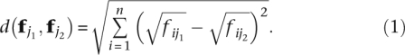 |
Both the Hellinger and the Euclidean distance between two arbitrary points on the n-standard simplex range between 0 and  for n ≥ 2. However, the Hellinger values compared with the Euclidean are comparatively higher for pairs of individuals nearest to the edges of the simplex, that is, with more extreme proportions, and, conversely, they are smaller for pairs near the center. For instance, in a gene with two splicing forms, the Euclidean distance between two individuals with proportions (0.5, 0.5) and (0.55, 0.45) is ∼0.071. The more extreme individuals (0.9, 0.1) and (0.95, 0.05) are also at Euclidean distance 0.071, while the Hellinger distances for the same two situations are, respectively, 0.050 and 0.096.
Anderson defines the multivariate dispersion of a given group of k individuals—in our case, the variability of the relative expressions—as the mean distance of the k points to its centroid cm:
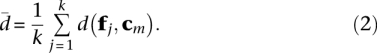 |
The centroid cm is defined by Anderson as the spatial median of the sampled points, that is, the point that minimizes the sum of distances between the sampled points. It shows better statistical properties than the vector of means, or even the vector of scalar medians (for further details, see Anderson 2006). In genes with similar splicing ratios across the individuals in the population, dispersion of the points around the centroid is minimal, and  tends to 0. As the differences in alternative splicing ratios between individuals increase,
  increases, tending to a maximum value. When k > n, it can be shown that
 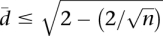 .
.
The meaning of the values of  can be more easily interpreted when compared with the values in a reference distribution. For that purpose, we have conducted a Monte Carlo simulation of
  , assuming random proportions of splicing isoforms, for different numbers of splicing isoforms ranging from n = 2 to n = 15. We have computed 1000 simulations (corresponding to 1000 genes) in each case assuming samples of k = 60 and k = 69 individuals. The proportions of the splicing isoforms have been drawn from a uniform distribution. The Monte Carlo distribution of
  provides us with reference values for the mean, median, standard deviation, and several percentiles (see Supplemental Fig. 2). These simulated distributions are symmetrical, showing a Gaussian-like shape. Interestingly, while the average variability increases with the number of splice forms, the range of variabilities decreases, with genes showing more homogeneous values of variability for a larger number of splice forms. Supplemental Figure 2 was designed to help understanding the meaning of the values of
  (see also Supplemental Methods). The computations are simulated in the simplified context of uniform random proportions over the standard simplex, assuming additionally independent values between individuals. The “true” distribution of
  is not known, and it is very unlikely that it will follow the uniform model, but our purpose is not to establish a model for
  , but only a reference model in conditions of total randomness. The observed values of
  seem to follow an asymmetrical distribution with a longer right tail and a second low peak. When compared with our reference distribution, most genes show less variability than expected from the independent random pulls.
We have also tested for homogeneity of the dispersion of splicing proportions across populations. We have used the Anderson distance-based test (Anderson 2006). This is more robust than the traditional likelihood test (for details, see Anderson 2006), and it can be easily combined with a permutation procedure that does not assume normality of the residuals. To reduce the false discovery rate, we have adjusted the P-values of the individual comparisons using the Benjamini and Hochberg approach (Benjamini and Hochberg 1995).
The method betadisper of the R package vegan (Oksanen et al. 2010) computes for a given gene the value of  for the two sampled populations and their homogeneity permutation test. By using the method p.adjust of the package stats, we can adjust the false discovery rate. Further details on the availability of the scripts used to compute
  can be found in the Supplemental Methods.
Identification of genes with population-specific splicing patterns
If variability of alternative splicing ratios is homogeneous between the two populations for a given gene, we could further test whether there is homogeneity of the splicing ratios themselves (and not of their variability as in the previous section). In other words, we can test for a given gene whether the splicing ratios within one population are homogeneous and different from the splicing ratios in the other population. This could be used to identify genes that have differential splicing in one population versus the other, that is, population-specific splicing ratios. Considering again the individuals geometrically embedded in an n -dimensional space (n = number of splice forms), we consequently use the non-parametric distance test described in Anderson (2001), with the Hellinger distance as a dissimilarity measure. The Anderson test is analogous to a multivariate analysis of variance without probabilistic distribution assumptions. The P-values of the individual gene comparisons are adjusted again using the Benjamini and Hochberg correction.
The method adonis of vegan (Oksanen et al. 2010) computes the Anderson test of homogeneity of splice forms for a given gene. The method p.adjust of the package stats adjusts the false discovery rate.
Quantifying the relative importance of variability in gene expression and variability in alternative splicing into individual transcript variability
While the coefficient of variation and the dispersion in the Hellinger distances proved appropriate to measure variability in gene expression and splicing ratios, from their direct comparison it is not possible to quantify their relative contribution to the observed variability in the total abundance of individual alternative splice forms. To address this issue, we propose here a multiplicative model, based on the calculation of two parameters: Vt and Vls (defined below).
Here we also follow a multivariate approach. Let's assume a gene with n splicing forms and the absolute abundances of these forms measured in k individuals. For each individual, these abundances can be represented by a point in ℝn, restricted here only to be in the positive orthant (these are all absolute abundance values). The measure most often used to describe scatter about the mean in multivariate data is the total variation (Seber 1984). This is the sum of the variances in the abundances of the alternative splice forms across the k individuals, or, more technically, the trace of the covariance matrix of the abundances of the alternative transcript isoforms. We refer to this sum of variances here as Vt. This is a quantity often used as a measure of variation in Principal Component Analysis: If the k points are projected on any subspace of ℝn, Vt is an upper bound of the dispersion of the projected points.
Let us assume an hypothetical gene with possibly different global expressions on the k individuals but constant splicing ratios. Denoting by λj the global expression of the j individual and by (f1, …, fn) the vector of constant splicing ratios, the absolute expression of the i splicing on the j individual is simply λjfi. In the geometrical representation, the k points corresponding to the abundances of the different splice forms from this gene in the different individuals in the population perfectly align on a line that follows the direction traced by the vector f = [fi]n×1 (Supplemental Fig. 4A). In general, any gene fitting exactly this model will include only points belonging to a line embedded in the full n-dimensional space. Obviously, if the model fits the data without error, the variations measured over the line and over the entire space are exactly the same.
In general, however, a gene will probably show differences between individuals in splicing ratios, and the points will not draw a line, but a complex n-dimensional scatterplot. Using the least squares criteria, we have obtained for this situation an analytical expression for the line of ℝn with non-negative coefficients that minimizes the distance between the original and the k projected points. In other words, we can express in a closed form the estimation of f and λ1, …, λn that better fits the n-values of alternative splice abundances, when a multiplicative model (of constant splicing ratios) is assumed. We refer to the variation of the projected points in this line as to Vls. In general, unless the points are originally already in a line, the projection will imply a loss of information—as data points are projected from n dimensions to 1—and the variability of the projected points (Vls) will be smaller than the original variability (Vt) (Supplemental Fig. 4B).
The projections on this straight line are linear transformations of the original alternative splice abundances, but we have demonstrated that it is not necessary to obtain their explicit values to obtain their variability. This can be easily obtained from the original abundance values (for technical details, see the Supplemental Methods).
The ratio (Vls/Vt) × 100, that is, the ratio of the variability in the projected line over the total variability, allows us to measure the adequacy of the multiplicative model in terms of the percentage of explained variability. It can be interpreted similarly to the R2 coefficient of the linear models or to the amount of variation explained by a subset of eigenvectors in Principal Component Analysis. For instance, a ratio close to 1 indicates that the multiplicative model, which assumes constant splicing ratios across individuals, explains almost all of the observed variability. That is, most of the variability in the abundances of the gene's alternatively splicing forms is the result of the variability in gene expression, and not of variability in splicing ratios. Conversely, a ratio close to 0 indicates that the multiplicative model fits the data poorly and that variability in gene expression explains little of the observed variability. One could thus assume that variability in splicing ratios is the major determinant of the observed variability in the abundances of alternative splice forms.
Further details on the availability of the scripts used to compute both Vls and Vt parameters can be found in the Supplemental Methods.
GO analysis
We used the DAVID software (Huang et al. 2009a,b) to investigate functional enrichment in four different gene sets: (1) the top 10% of genes with the highest Vls/Vt, that is, genes in which most variability can be attributed to changes in transcription; (2) the top 10% of genes with lowest Vls/Vt, genes in which most variability can be attributed to splicing; (3) the 10% of genes with the lowest Vt; and (4) the 10% of genes with the highest Vt. For each category, we considered only the genes common to both populations and set a false discovery rate of <5% and a P-value inferior to 0.05 as thresholds for the identification of significantly over-represented GO terms. The reference population was defined by all genes taken into account in this study (i.e., common genes in the two populations that passed the filters specified in Table 2). Additionally, we used the same approach for the set of 44 genes in which one isoform is uniquely used in one population (i.e., expressed in all the individuals) and a different one is uniquely used in the other population.
Splicing factors
A total of 309 genes related to RNA splicing were identified through the database AmiGO (version 1.7) (Carbon et al. 2009), 201 of which were found expressed in all individuals and used in the analyses.
Data access
Flux Capacitor quantifications for genes and transcripts in the Caucasian and Yoruban populations, as well as the scripts used in this paper, can be found online at http://big.crg.cat/bioinformatics_and_genomics/SplicingVariability.
Acknowledgments
We thank Hagen Tilgner, Maria Ortiz, David Gonzalez, and Alvis Brazma's group for useful discussions and help with the data. We also thank the reviewers for their constructive comments. This work has been carried out under grants RD07/0067/0012, BIO2006-03380, CSD2007-00050, and MTM2008-00642 from the Spanish Ministry of Science; grant SGR-1430 from the Catalan Government; grants 1U54HG004557-01 and 1U54HG004555-01 from the National Institutes of Health; and INB-ISCIII from Instituto de Salud Carlos III and FEDER.
Footnotes
[Supplemental material is available for this article.]
Article published online before print. Article, supplemental material, and publication date are at http://www.genome.org/cgi/doi/10.1101/gr.121947.111.
References
- Anderson MJ 2001. A new method for non parametric multivariate analysis of variance. Austral Ecol 26: 32–46 [Google Scholar]
- Anderson MJ 2006. Distance-based tests for homogeneity of multivariate dispersions. Biometrics 62: 245–253 [DOI] [PubMed] [Google Scholar]
- Benjamini Y, Hochberg Y 1995. Controlling the false discovery rate: A practical and powerful approach to multiple testing. J R Stat Soc Ser B Methodol 57: 289–300 [Google Scholar]
- Bentley DL 2005. Rules of engagement: Co-transcriptional recruitment of pre-mRNA processing factors. Curr Opin Cell Biol 17: 251–256 [DOI] [PubMed] [Google Scholar]
- Carbon S, Ireland A, Mungall CJ, Shu S, Marshall B, Lewis S 2009. AmiGO: Online access to ontology and annotation data. Bioinformatics 25: 288–289 [DOI] [PMC free article] [PubMed] [Google Scholar]
- Cloonan N, Forrest ARR, Kolle G, Gardiner BBA, Faulkner GJ, Brown MK, Taylor DF, Steptoe AL, Wani S, Bethel G, et al. 2008. Stem cell transcriptome profiling via massive-scale mRNA sequencing. Nat Methods 5: 613–619 [DOI] [PubMed] [Google Scholar]
- Harrow J, Denoeud F, Frankish A, Reymond A, Chen C, Chrast J, Lagarde J, Gilbert JGR, Storey R, Swarbreck D et al. 2006. GENCODE: Producing a reference annotation for ENCODE. Genome Biol 7 Suppl 1: S4.1–S4.9 [DOI] [PMC free article] [PubMed] [Google Scholar]
- Huang DW, Sherman BT, Lempicki RA 2009a. Bioinformatics enrichment tools: Paths toward the comprehensive functional analysis of large gene lists. Nucleic Acids Res 37: 1–13 [DOI] [PMC free article] [PubMed] [Google Scholar]
- Huang DW, Sherman BT, Lempicki RA 2009b. Systematic and integrative analysis of large gene lists using DAVID bioinformatics resources. Nat Protoc 4: 44–57 [DOI] [PubMed] [Google Scholar]
- International HapMap Consortium 2003. The international HapMap project. Nature 426: 789–796 [DOI] [PubMed] [Google Scholar]
- International HapMap Consortium 2005. A haplotype map of the human genome. Nature 437: 1299–1320 [DOI] [PMC free article] [PubMed] [Google Scholar]
- International HapMap Consortium 2007. A second generation human haplotype map of over 3.1 million SNPs. Nature 449: 851–861 [DOI] [PMC free article] [PubMed] [Google Scholar]
- International HapMap 3 Consortium, Altshuler DM, Gibbs RA, Peltonen L, Altshuler DM, Gibbs RA, Peltonen L, Dermitzakis E, Schaffner SF, Yu F, Peltonen L, et al. 2010. Integrating common and rare genetic variation in diverse human populations. Nature 467: 52–58 [DOI] [PMC free article] [PubMed] [Google Scholar]
- Jiang H, Wong WH 2009. Statistical inferences for isoform expression in RNA-Seq. Bioinformatics 25: 1026–1032 [DOI] [PMC free article] [PubMed] [Google Scholar]
- Kornblihtt AR 2007. Coupling transcription and alternative splicing. Adv Exp Med Biol 623: 175–189 [DOI] [PubMed] [Google Scholar]
- Lalonde E, Ha KCH, Wang Z, Bemmo A, Kleinman CL, Kwan T, Pastinen T, Majewski J 2011. RNA sequencing reveals the role of splicing polymorphisms in regulating human gene expression. Genome Res 21: 545–554 [DOI] [PMC free article] [PubMed] [Google Scholar]
- Legendre P, Gallagher ED 2001. Ecologically meaningful transformations for ordination of species data. Oecologia 129: 271–280 [DOI] [PubMed] [Google Scholar]
- Li J, Liu Y, Kim T, Min R, Zhang Z 2010. Gene expression variability within and between human populations and implications toward disease susceptibility. PLoS Comput Biol 6: e1000910 doi: 10.1371/journal.pcbi.1000910 [DOI] [PMC free article] [PubMed] [Google Scholar]
- Marioni JC, Mason CE, Mane SM, Stephens M, Gilad Y 2008. RNA-seq: An assessment of technical reproducibility and comparison with gene expression arrays. Genome Res 18: 1509–1517 [DOI] [PMC free article] [PubMed] [Google Scholar]
- Montgomery SB, Sammeth M, Gutierrez-Arcelus M, Lach RP, Ingle C, Nisbett J, Guigo R, Dermitzakis ET 2010. Transcriptome genetics using second generation sequencing in a Caucasian population. Nature 464: 773–777 [DOI] [PMC free article] [PubMed] [Google Scholar]
- Mortazavi A, Williams BA, McCue K, Schaeffer L, Wold B 2008. Mapping and quantifying mammalian transcriptomes by RNA-Seq. Nat Methods 5: 621–628 [DOI] [PubMed] [Google Scholar]
- Nagalakshmi U, Wang Z, Waern K, Shou C, Raha D, Gerstein M, Snyder M 2008. The transcriptional landscape of the yeast genome defined by RNA sequencing. Science 320: 1344–1349 [DOI] [PMC free article] [PubMed] [Google Scholar]
- Oksanen J, Blanchet FG, Kindt R, Legendre P, O'Hara RB, Simpson GL, Solymos P, Stevens MHH, Wagner, H 2010. vegan: Community Ecology Package. R package version 1.18-16/r1371. http://cran.r-project.org/web/packages/vegan/index.html
- Pandit S, Wang D, Fu X 2008. Functional integration of transcriptional and RNA processing machineries. Curr Opin Cell Biol 20: 260–265 [DOI] [PMC free article] [PubMed] [Google Scholar]
- Pickrell JK, Marioni JC, Pai AA, Degner JF, Engelhardt BE, Nkadori E, Veyrieras J, Stephens M, Gilad Y, Pritchard JK 2010. Understanding mechanisms underlying human gene expression variation with RNA sequencing. Nature 464: 768–772 [DOI] [PMC free article] [PubMed] [Google Scholar]
- Ponting CP, Oliver PL, Reik W 2009. Evolution and functions of long noncoding RNAs. Cell 136: 629–641 [DOI] [PubMed] [Google Scholar]
- Rao C 1995. A review of canonical coordinates and an alternative to correspondence analysis using Hellinger distance. Qüestiió 19: 23–63 [Google Scholar]
- Seber G 1984. Multivariate observations. Wiley, New York [Google Scholar]
- Spielman RS, Bastone LA, Burdick JT, Morley M, Ewens WJ, Cheung VG 2007. Common genetic variants account for differences in gene expression among ethnic groups. Nat Genet 39: 226–231 [DOI] [PMC free article] [PubMed] [Google Scholar]
- Storey JD, Madeoy J, Strout JL, Wurfel M, Ronald J, Akey JM 2007. Gene-expression variation within and among human populations. Am J Hum Genet 80: 502–509 [DOI] [PMC free article] [PubMed] [Google Scholar]
- Stranger BE, Nica AC, Forrest MS, Dimas A, Bird CP, Beazley C, Ingle CE, Dunning M, Flicek P, Koller D, et al. 2007. Population genomics of human gene expression. Nat Genet 39: 1217–1224 [DOI] [PMC free article] [PubMed] [Google Scholar]
- Sultan M, Schulz MH, Richard H, Magen A, Klingenhoff A, Scherf M, Seifert M, Borodina T, Soldatov A, Parkhomchuk D, et al. 2008. A global view of gene activity and alternative splicing by deep sequencing of the human transcriptome. Science 321: 956–960 [DOI] [PubMed] [Google Scholar]
- Trapnell C, Williams BA, Pertea G, Mortazavi A, Kwan G, van Baren MJ, Salzberg SL, Wold BJ, Pachter L 2010. Transcript assembly and quantification by RNA-Seq reveals unannotated transcripts and isoform switching during cell differentiation. Nat Biotechnol 28: 511–515 [DOI] [PMC free article] [PubMed] [Google Scholar]
- Veyrieras J, Kudaravalli S, Kim SY, Dermitzakis ET, Gilad Y, Stephens M, Pritchard JK 2008. High-resolution mapping of expression-QTLs yields insight into human gene regulation. PLoS Genet 4: e1000214 doi: 10.1371/journal.pgen.1000214 [DOI] [PMC free article] [PubMed] [Google Scholar]
- Wang ET, Sandberg R, Luo S, Khrebtukova I, Zhang L, Mayr C, Kingsmore SF, Schroth GP, Burge CB 2008. Alternative isoform regulation in human tissue transcriptomes. Nature 456: 470–476 [DOI] [PMC free article] [PubMed] [Google Scholar]
- Wilhelm BT, Marguerat S, Watt S, Schubert F, Wood V, Goodhead I, Penkett CJ, Rogers J, Bähler J 2008. Dynamic repertoire of a eukaryotic transcriptome surveyed at single-nucleotide resolution. Nature 453: 1239–1243 [DOI] [PubMed] [Google Scholar]
- Zhang W, Duan S, Bleibel WK, Wisel SA, Huang RS, Wu X, He L, Clark TA, Chen TX, Schweitzer AC, et al. 2009. Identification of common genetic variants that account for transcript isoform variation between human populations. Hum Genet 125: 81–93 [DOI] [PMC free article] [PubMed] [Google Scholar]
- Zheng S, Chen L 2009. A hierarchical Bayesian model for comparing transcriptomes at the individual transcript isoform level. Nucleic Acids Res 37: e75 doi: 10.1093/nar/gkp282 [DOI] [PMC free article] [PubMed] [Google Scholar]