Approximation for Cooperative Interactions of a Spatially-Detailed Cardiac Sarcomere Model

Abstract

We developed a novel ordinary differential equation (ODE) model, which produced results that correlated well with the Monte Carlo (MC) simulation when applied to a spatially-detailed model of the cardiac sarcomere. Configuration of the novel ODE model was based on the Ising model of myofilaments, with the “co-operative activation” effect introduced to incorporate nearest-neighbor interactions. First, a set of parameters was estimated using arbitrary Ca transient data to reproduce the combinational probability for the states of three consecutive regulatory units, using single unit probabilities for central and neighboring units in the MC simulation. The parameter set thus obtained enabled the calculation of the state transition of each unit using the ODE model with reference to the neighboring states. The present ODE model not only provided good agreement with the MC simulation results but was also capable of reproducing a wide range of experimental results under both steady-state and dynamic conditions including shortening twitch. The simulation results suggested that the nearest-neighbor interaction is a reasonable approximation of the cooperativity based on end-to-end interactions. Utilizing the modified ODE model resulted in a reduction in computational costs but maintained spatial integrity and co-operative effects, making it a powerful tool in cardiac modeling.

Introduction

Mathematical modeling is an indispensable tool in defining the mechanisms of activation and force generation of the cardiac sarcomere. Various mathematical models have been designed to replicate and characterize the cellular processes and activities of the sarcomere and, recently, detailed structure and filament properties have also been taken into account.2,4,10,16 However, current models have yet to replicate the anomalously high sensitivity of developed force to changes in the free cytosolic calcium (Ca) concentration, observed under both steady-state and dynamic conditions. This aberrant effect is suggested to be brought about by the “co-operative” interactions among intracellular molecules within the sarcomere. One postulated mechanism of “cooperativity” suggests that the strongly-bound cross-bridge releases the steric hindrance of tropomyosin to facilitate the attachment of nearby cross-bridges. A further potential mechanism underlying the “co-operative” interactions is the end-to-end interactions of regulatory troponin/tropomyosin (T/T) units along the thin filament. In either case, the physical arrangement of each molecular component is suggested to be a critical factor.

To reproduce the “co-operative” effects that occur within the sarcomere, most current models utilize the “phenomenological parameter tuning strategy” to normalize the behavior of cross-bridges and to avoid the necessity of determining the state of each regulatory unit and the interactions among them (mean-field approximation). Although this approach enables the use of ordinary differential equations (ODE), has a lower computational cost, and has been reported to provide a fairly good representation of experimental data,1,9,13,20,21 the models lack a representation of spatial activity within the cell. This limits the predictive ability of the models and hampers the potential for direct comparisons with experimentally obtained data.18

Spatially-distributed models have been proposed that are capable of mimicking the physical arrangement of each functional unit within a cell, including the cross-bridges in the thick and thin filaments of the sarcomere.8,10,19,22 In these models, the transition rates of each unit are dependent on the states of neighboring units and/or the cross-bridge strain to reveal any potential “co-operative” mechanisms that occur. Moreover, the models have been found to have excellent reproducibility. However, the inherent and inevitable problem with this type of model is the necessity of using the computationally expensive Monte Carlo (MC) simulation. Although Rice et al.19 reported an analytical solution to their Ising model of myofilaments without MC simulation, its application is limited to the static state with a simple periodic boundary condition. Very recently, Campbell et al.3 proposed a Markov model approach to represent the states of regulatory units, but the computational costs again limited the number of units studied in the model.

Here we propose a novel method for describing the behavior of a spatially detailed co-operative model using ODE in which the regulatory units are distributed along the sarcomere filament. Through modifications to the Ising model produced by Rice et al.,19 we produced an ODE model that is applicable to a wider range of experimental conditions, including accounting for changes in sarcomere length (SL). Our modified ODE model was found to correlate well with the MC simulation over a wide range of dynamically changing Ca concentrations. Moreover, our ODE model is capable of recording the information of neighboring units and reproducing the co-operative phenomenon arising from molecular interactions along the sarcomere filaments. Importantly, this novel ODE model is associated with greatly reduced computational costs, thereby enabling its application for large scale models of cardiac physiology.

Methods

Description of the Model

The sarcomere model used in the present study is illustrated in Fig. 1. The model consists of a pair of thin filaments (AF) and a single thick filament (MF). Myosin heads (MHs) are arranged symmetrically on the thick filament with regular intervals on both sides of the bare-zone (B-zone). The geometry of the model is summarized in Table 1. To introduce SL as a factor in the model, we assigned a functional unit to each MH coupled with the opposing segment of thin filament and indexed as “i”. This process conflicts somewhat with the traditional practices used in sarcomere modeling where the unit is commonly placed on the thin filament. However, because the helical pitch of the myosin filament is close to that of actin (composed of seven monomeric actins) and regulated by a single troponin/tropomyosin (T/T) complex, we believe this strategy is rational. The model was assumed to be symmetrical, and simulation was performed on half of one sarcomere.

Figure 1.

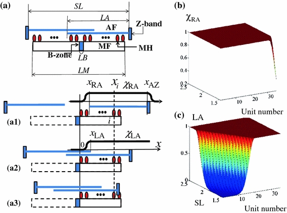
Schematic of the sarcomere model (a). (a1) Relative position of filaments in the single overlapping state (SL > 2LA + LB). x _RA: position of the end of the right thin filament, x _AZ: position of Z-band of the right thin filament, x_i: position of i _th MH, both measured from the right-hand edge of the bare zone. (a2) The double overlapping state (LM < SL < 2LA − LB). x _LA: position of the end of the left thin filament. (a3) State of no overlapping at the MF ends (SL < LM). MF: thick filament, MH: myosin head, B-zone: bare zone, AF: thin filament, SL: sarcomere length LA: thin filament length, LM: thick filament length, LB: bare zone length. Dependence of the lumped parameters χ _RA(SL, i) (b) and χ _LA(SL, i) (c) on SL at individual unit (MH_i)

Table 1.

Model parameters

Parameter	Value	Units
Sarcomere geometry
LA (length of AF)	1.2	μm	*
LM (length of MF)	1.65	μm	*
LB (length of B-zone)	0.1	μm	*
nu (number of MHs)	36	Unitless	*
Transition rates Ca-bound
K on	80	μM−1 s−1	**
K off	80	s−1	**
\documentclass[12pt]{minimal} \usepackage{amsmath} \usepackage{wasysym} \usepackage{amsfonts} \usepackage{amssymb} \usepackage{amsbsy} \usepackage{mathrsfs} \usepackage{upgreek} \setlength{\oddsidemargin}{-69pt} \begin{document}$$ K^{\prime}_{\text{on}} $$\end{document}	80	μM−1 s−1	**
\documentclass[12pt]{minimal} \usepackage{amsmath} \usepackage{wasysym} \usepackage{amsfonts} \usepackage{amssymb} \usepackage{amsbsy} \usepackage{mathrsfs} \usepackage{upgreek} \setlength{\oddsidemargin}{-69pt} \begin{document}$$ K^{\prime}_{\text{off}} $$\end{document}	8	s−1	**
Transition rates N–P			**
Q 0	3	Unitless	**
SL Q	2.2	μm	**
α Q	1.4	μm−1	**
K basic	10	s−1	**
μ	10	Unitless	**
γ	40	Unitless	**
SL dependence
a R	0.1	μm
a L	0.1	μm
Time interval lengths
DT (for averaging in MC)	2.5	ms
Δt	2.5	μs

Parameter values were adopted * from Rice et al.,20 ** from Rice et al.19 with modifications

The co-operative four-state Markov model proposed by Rice et al.19 was adopted for the present model whereby the state of each functional unit is characterized by the combination of Ca binding (1: bound, 0: not bound) and cross-bridge formation (P: permitted, N: not permitted; Fig. 2). To introduce the co-operative mechanisms occurring in force generation, the factors γ ⁿ and γ ⁻ⁿ were multiplied by the transition rates from N to P and from P to N, respectively, where n (=0, 1 or 2) is the number of nearest-neighboring MHs in the P-state.

Figure 2.

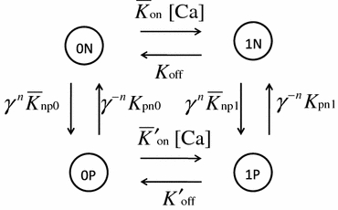
The cooperative four-state Markov model. States are coded with the combination of the Ca binding state (0: not bound, 1: bound) and conformation for cross-bridge formation (P: permissive, N: non-permissive). Transitions among the states are governed by the rate constant adjacent to each arrow. To introduce the co-operative behavior for the transition between states P and N, the factors γ ⁿ and γ ⁻ⁿ are multiplied by the transition rates from N to P and P to N, respectively, where n is the number of neighboring MHs in the P-state. The overlines for transition rates \documentclass[12pt]{minimal} \usepackage{amsmath} \usepackage{wasysym} \usepackage{amsfonts} \usepackage{amssymb} \usepackage{amsbsy} \usepackage{mathrsfs} \usepackage{upgreek} \setlength{\oddsidemargin}{-69pt} \begin{document}$$ \bar{K}_{{{\text{np}}0}},\;\bar{K}_{{{\text{np}}1}} ,\;\bar{K}_{\text{on}} $$\end{document} and \documentclass[12pt]{minimal} \usepackage{amsmath} \usepackage{wasysym} \usepackage{amsfonts} \usepackage{amssymb} \usepackage{amsbsy} \usepackage{mathrsfs} \usepackage{upgreek} \setlength{\oddsidemargin}{-69pt} \begin{document}$$ \bar{K}^{\prime}_{\text{on}} $$\end{document} indicate that these rates are modified according to the SL. [Ca] denotes the free Ca concentration

In addition, we modified the following rate constants by multiplying the geometrical factors χ_RA(SL,i) and χ_LA(SL,i) (Figs. 1A1, A2, 1B and 1C) to introduce a dependence on the filament overlap determined by SL:

\documentclass[12pt]{minimal} \usepackage{amsmath} \usepackage{wasysym} \usepackage{amsfonts} \usepackage{amssymb} \usepackage{amsbsy} \usepackage{mathrsfs} \usepackage{upgreek} \setlength{\oddsidemargin}{-69pt} \begin{document}\bar{K}_{{{\text{np}}0}} \left( {SL,i} \right) = \chi_{\text{LA}} \left( {SL,i} \right)\chi_{\text{RA}} \left( {SL,i} \right)K_{{{\text{np}}0}},\\\;\bar{K}_{{{\text{np}}1}} \left( {SL,i} \right) = \chi_{\text{LA}} \left( {SL,i} \right)\chi_{\text{RA}} \left( {SL,i} \right)K_{{{\text{np}}1}} ,\\\;\bar{K}_{\text{on}} \left( {SL,i} \right) = \chi_{\text{RA}} \left( {SL,i} \right)K_{\text{on}},\\\;\bar{K}^{\prime}_{\text{on}} \left( {SL,i} \right) = \chi_{\text{RA}} \left( {SL,i} \right)K^{\prime}_{\text{on}}.\end{document} 1

The factors χ_RA(SL,i) and χ_LA(SL,i) were defined for each unit as the function of its position (x _i) and the degree of filament overlap, determined by the positions of two thin filament ends (the free end (x _RA) of the right-hand side filament, the Z-band (x _AZ) of the right-hand side filament and the free end (x _LA) of the left-hand side filament) (Fig. 1).

\documentclass[12pt]{minimal} \usepackage{amsmath} \usepackage{wasysym} \usepackage{amsfonts} \usepackage{amssymb} \usepackage{amsbsy} \usepackage{mathrsfs} \usepackage{upgreek} \setlength{\oddsidemargin}{-69pt} \begin{document}$$ x_{\text{AZ}} = \left( {SL - LB} \right)/2,\;x_{\text{LA}} = LA - x_{\text{AZ}} - LB,\;x_{\text{RA}} = x_{\text{AZ}} - LA. $$\end{document} 2

When there are non-overlapping regions of the two filaments (SL > 2LA + LB, Fig. 1A1), only the units where x _i > x _RA can form cross-bridges without the modification to the rate constant. For those cross-bridges located in non-overlapping regions (x _i ≤ x _RA), the rate constant becomes attenuated as the distance to the MH extends further from the thin filament end:

\documentclass[12pt]{minimal} \usepackage{amsmath} \usepackage{wasysym} \usepackage{amsfonts} \usepackage{amssymb} \usepackage{amsbsy} \usepackage{mathrsfs} \usepackage{upgreek} \setlength{\oddsidemargin}{-69pt} \begin{document}$$ \chi_{\text{RA}} \left( {SL,i} \right)=\left\{\begin{array}{ll}\exp \left( - \left( x_{\text{RA}} - x_{i} \right)^{2}/a_{\text{R}}^{2} \right), & x_{i} \le x_{\text{RA}} \\ 1, & x_{\text{RA}} < x_{i} < x_{\text{AZ}}\\ \exp \left( { - \left({x_{i} - x_{\text{AZ}} } \right)^{2} /a_{\text{R}}^{2} } \right),& x_{i} \ge x_{\text{AZ}}\end{array} \right.,$$\end{document} 3

where a step function is smoothed at the ends so that χ _RA changes continuously with respect to SL. The third condition of Eq. (3) becomes effective for determining \documentclass[12pt]{minimal} \usepackage{amsmath} \usepackage{wasysym} \usepackage{amsfonts} \usepackage{amssymb} \usepackage{amsbsy} \usepackage{mathrsfs} \usepackage{upgreek} \setlength{\oddsidemargin}{-69pt} \begin{document}$$ \bar{K}_{{{\text{np}}0}} $$\end{document} and \documentclass[12pt]{minimal} \usepackage{amsmath} \usepackage{wasysym} \usepackage{amsfonts} \usepackage{amssymb} \usepackage{amsbsy} \usepackage{mathrsfs} \usepackage{upgreek} \setlength{\oddsidemargin}{-69pt} \begin{document}$$ \bar{K}_{{{\text{np}}1}} $$\end{document} in Eq. (1) when no overlapping state appears at the right ends of MF (Fig. 1A3). The genesis of the ascending limb in the force–length relation in regions of SL shorter than the optimal length is a controversial issue. For this model, we assumed that the formation of the cross-bridge was inhibited for MHs in the double overlap region of the thin filament (Fig. 1A2, SL < 2LA − LB):

\documentclass[12pt]{minimal} \usepackage{amsmath} \usepackage{wasysym} \usepackage{amsfonts} \usepackage{amssymb} \usepackage{amsbsy} \usepackage{mathrsfs} \usepackage{upgreek} \setlength{\oddsidemargin}{-69pt} \begin{document}$$ \chi_{\text{LA}} \left( {SL,i} \right) = \left\{\begin{array}{ll} \exp \left( - \left({x_{\text{LA}} - x_{i}} \right)^{2} /a_{\text{L}}^{2} \right), & x_{i} \le x_{\text{LA}} \\ {1,} & x_{i} > x_{\text{LA}} \\ \end{array} \right.. $$\end{document} 4

The parameters a _R and a _L determine how rapidly the MHs at the borders of overlapping zone lose their capability to form attached bridges as they become distant from the filament ends. The values were adjusted to agree with the experimental force–length relation and are listed in Table 1. Finally, the MHs at the edges of the filament (i = 1 and nu) were assumed to always have N-state neighbors on their null side.

Monte Carlo Simulation

The MC simulation was performed according to the following rules. For a given random number r ∈ [0, 1] generated for each unit (ith MH) at each time interval ([t, t + Δt]), the state ^t α _i (either 0N, 1N, 0P, or 1P) at time t transitions to the new state \documentclass[12pt]{minimal} \usepackage{amsmath} \usepackage{wasysym} \usepackage{amsfonts} \usepackage{amssymb} \usepackage{amsbsy} \usepackage{mathrsfs} \usepackage{upgreek} \setlength{\oddsidemargin}{-69pt} \begin{document}$$ {}^{t + \Updelta t}\alpha_{i} = T_{\Updelta t} \left( {{}^{t}\alpha_{i} } \right) $$\end{document} during the time interval [t, t + Δt] at all MHs as follows:

\documentclass[12pt]{minimal} \usepackage{amsmath} \usepackage{wasysym} \usepackage{amsfonts} \usepackage{amssymb} \usepackage{amsbsy} \usepackage{mathrsfs} \usepackage{upgreek} \setlength{\oddsidemargin}{-69pt} \begin{document}$$ \begin{aligned} T_{\Updelta t} \left( {0{\text{N}}} \right) &= \left\{\begin{array} {ll} 1{\text{N}}, & 0 \le r < \Updelta t\bar{K}_{\text{on}} \left[ {\text{Ca}} \right]\\ 0{\text{P}}, & \Updelta t\bar{K}_{\text{on}} \left[ {\text{Ca}} \right] \le r < \Updelta t\left( {\bar{K}_{\text{on}} \left[ {\text{Ca}} \right] + \gamma^{n} \bar{K}_{{{\text{np}}0}} } \right)\\ 0{\text{N}}, & \Updelta t\left( {\bar{K}_{\text{on}} \left[ {\text{Ca}} \right] + \gamma^{n} K_{{{\text{np}}0}} } \right) \le r \le 1 \\ \end{array} \right. \\ T_{\Updelta t} \left( {1{\text{N}}} \right) &= \left\{\begin{array}{ll} 0{\text{N}}, & 0 \le r < \Updelta tK_{\text{off}}\\ 1{\text{P}}, & \Updelta tK_{\text{off}} \le r < \Updelta t\left( {K_{\text{off}} + \gamma^{n} \bar{K}_{{{\text{np}}1}} } \right)\\ 1{\text{N}}, & \Updelta t\left( {K_{\text{off}} + \gamma^{n} \bar{K}_{{{\text{np}}1}} } \right) \le r \le 1 \end{array} \right. \\ T_{\Updelta t} \left( {1{\text{P}}} \right) &= \left\{\begin{array}{ll} 1{\text{N}}, & 0 \le r < \Updelta t\gamma^{ - n} K_{{{\text{pn}}1}}\\ 0{\text{P}},& \Updelta t\gamma^{ - n} K_{{{\text{pn}}1}} \le r < \Updelta t\left( {\gamma^{ - n} K_{{{\text{pn}}1}} + K^{\prime}_{\text{off}} } \right)\\ 1{\text{P}}, & \Updelta t\left( {\gamma^{ - n}K_{{{\text{pn}}1}} + K^{\prime}_{\text{off}} } \right) \le r \le 1 \end{array} \right. \\ T_{\Updelta t} \left( {0{\text{P}}} \right) &= \left\{\begin{array}{ll} 1{\text{P}}, & 0 \le r < \Updelta tK^{\prime}_{\text{on}} \left[ {\text{Ca}} \right]\\ 0{\text{N}}, & \Updelta t\bar{K}^{\prime}_{\text{on}} \left[ {\text{Ca}} \right] \le r < \Updelta t\left( {\bar{K}^{\prime}_{\text{on}} \left[ {\text{Ca}} \right] + \gamma^{ - n} K_{{{\text{pn}}0}} } \right)\\ 0{\text{P}},& \Updelta t\left({\bar{K}^{\prime}_{\text{on}} \left[ {\text{Ca}} \right] + \gamma^{ - n} K_{{{\text{pn}}0}} } \right) \le r \le 1 \end{array} \right. \end{aligned} $$\end{document}

The time interval Δt was chosen so that none of the values with the coefficient Δt in the third condition of each rule set exceeds 1. The parameter n is the number of nearest-neighboring MHs (i − 1th and i + 1th MHs) in the P-state at time t.

These transition rate constants were adopted from Rice et al.19 and modified. Some transition rates between the P-state and N-state were calculated with the parameters Q, K _basic, μ and γ (Table 1) as follows:

\documentclass[12pt]{minimal} \usepackage{amsmath} \usepackage{wasysym} \usepackage{amsfonts} \usepackage{amssymb} \usepackage{amsbsy} \usepackage{mathrsfs} \usepackage{upgreek} \setlength{\oddsidemargin}{-69pt} \begin{document}$$ K_{{{\text{np}}0}} = QK_{\text{basic}} /\mu ,\;K_{{{\text{np}}1}} = QK_{\text{basic}} ,\;K_{{{\text{pn}}0}} = K_{\text{basic}} \gamma^{2} ,\;K_{{{\text{pn}}1}} = K_{\text{basic}} \gamma^{2} ,\; K^{\prime}_{\text{on}} = K_{\text{on}} ,\;K^{\prime}_{\text{off}} = K_{\text{off}} /\mu.$$\end{document} 5

To reproduce the SL dependence of [Ca₅₀] on force–pCa relations,5,14 we introduced the SL dependence of Q. We found that the best results were obtained with the Q value decreasing from Q ₀ = 3 linearly with inclination α_Q = 1.4 μm⁻¹ as the SL becomes shorter from SL _Q = 2.2 μm.

\documentclass[12pt]{minimal} \usepackage{amsmath} \usepackage{wasysym} \usepackage{amsfonts} \usepackage{amssymb} \usepackage{amsbsy} \usepackage{mathrsfs} \usepackage{upgreek} \setlength{\oddsidemargin}{-69pt} \begin{document}$$ Q\left( {SL} \right) = \left\{ \begin{array}{ll} {Q_{0} ,} & {SL \ge SL_{\text{Q}} } \\ Q_{0} - \alpha_{Q} \left({SL_{\text{Q}} - SL} \right), & {SL < SL_{\text{Q}} } \\ \end{array} \right. $$\end{document} 6

The parameter values are summarized in Table 1.

Approximation by the ODE Model

There are 4^nu combinatory states for the model consisting of nu regulatory units. First, we introduced a linear ODE that gives the transitions of probability distribution of these combinatory states for a given Ca transient. This ODE provides a probability distribution that correlated well with the previously described MC simulation. However, the direct solution of this ODE is impractical because of the large number of degrees of freedom (4^nu with nu = 36 in our case). Therefore, we introduced a reduced ODE to obtain the averaged probability of the four states at each regulatory unit for the solution of the original ODE.

Each of the four states is represented by four integers:

\documentclass[12pt]{minimal} \usepackage{amsmath} \usepackage{wasysym} \usepackage{amsfonts} \usepackage{amssymb} \usepackage{amsbsy} \usepackage{mathrsfs} \usepackage{upgreek} \setlength{\oddsidemargin}{-69pt} \begin{document}$$ 0{\text{N}} \leftrightarrow 1,\;1{\text{N}} \leftrightarrow 2,\;1{\text{P}} \leftrightarrow 3,\;0{\text{P}} \leftrightarrow 4 $$\end{document} 7

The probability distribution “P” can then be represented as a linear combination of the 4^nu combinatory states:

\documentclass[12pt]{minimal} \usepackage{amsmath} \usepackage{wasysym} \usepackage{amsfonts} \usepackage{amssymb} \usepackage{amsbsy} \usepackage{mathrsfs} \usepackage{upgreek} \setlength{\oddsidemargin}{-69pt} \begin{document}$$ {\mathbf{P}} = \sum\limits_{{1 \le k_{1} \ldots k_{nu} \le 4}} {P\left( {k_{1} , \ldots ,k_{nu} } \right)\;{\mathbf{e}}\left( {k_{1} , \ldots ,k_{nu} } \right)} , $$\end{document} 8

The following conditions are fulfilled for the coefficients.

\documentclass[12pt]{minimal} \usepackage{amsmath} \usepackage{wasysym} \usepackage{amsfonts} \usepackage{amssymb} \usepackage{amsbsy} \usepackage{mathrsfs} \usepackage{upgreek} \setlength{\oddsidemargin}{-69pt} \begin{document}$$ \sum\limits_{{1 \le k_{1} \ldots k_{nu} \le 4}} {P\left( {k_{1} , \ldots ,k_{nu} } \right)} = 1,\;\;P\left( {k_{1} , \ldots ,k_{nu} } \right) \ge 0 $$\end{document} 9

Here, the basis vector e(k ₁,…,k _nu) corresponds to the combinatory states of nu units given in Eq. (7), and P(k ₁,…,k _nu) is interpreted as the probability of the total number of units to take this combinatory state.

The vector space representing probability distributions is composed of m = 4^nu basis vectors. Because we require nu = 36, the dimension m becomes so large that a single vector cannot be stored in the memory of a common computer. However, the transition kinetics of the probability distribution can be expressed by a simple linear ODE as follows.

For any given time t, we define a linear transformation ^t A that represents the transition kinetics at time t for the combinatory states by giving its action on the basis vectors:

\documentclass[12pt]{minimal} \usepackage{amsmath} \usepackage{wasysym} \usepackage{amsfonts} \usepackage{amssymb} \usepackage{amsbsy} \usepackage{mathrsfs} \usepackage{upgreek} \setlength{\oddsidemargin}{-69pt} \begin{document}$$ {}^{t}{\mathbf{A}} \cdot {\mathbf{e}}\left( {k_{1} , \ldots ,k_{nu} } \right) = \sum\limits_{1 \le i \le nu} {\sum\limits_{1 \le l \le 4} {{}^{t}A_{i} \left( {\psi \left( {k_{i - 1} } \right),\psi \left( {k_{i + 1} } \right)} \right)_{{l,k_{i} }} {\mathbf{e}}\left( {k_{1} , \ldots ,k_{i - 1} ,l,k_{i + 1} , \ldots ,k_{nu} } \right)} } , $$\end{document} 10

where ψ indicates the N- or P-state by

\documentclass[12pt]{minimal} \usepackage{amsmath} \usepackage{wasysym} \usepackage{amsfonts} \usepackage{amssymb} \usepackage{amsbsy} \usepackage{mathrsfs} \usepackage{upgreek} \setlength{\oddsidemargin}{-69pt} \begin{document}$$ \psi \left( 1 \right) = {\text{N}},\psi \left( 2 \right) = {\text{N}},\psi \left( 3 \right) = {\text{P}},\psi \left( 4 \right) = {\text{P}}. $$\end{document} 11

^t A _i(ξ, η)_l,k is the (l,k)-component of the 4 × 4 matrix given by

\documentclass[12pt]{minimal} \usepackage{amsmath} \usepackage{wasysym} \usepackage{amsfonts} \usepackage{amssymb} \usepackage{amsbsy} \usepackage{mathrsfs} \usepackage{upgreek} \setlength{\oddsidemargin}{-69pt} \begin{document}$$ {}^{t}{\mathbf{A}}_{i} \left( {\xi ,\eta } \right) = \left[\begin{array}{llll} - \bar{K}_{\text{on}} {}^{t}\left[{\text{Ca}} \right] - \gamma^{n} \bar{K}_{{{\text{np}}0}} &{K_{\text{off}} } & 0 & {\gamma^{ - n} K_{{{\text{pn}}0}} } \\ {\bar{K}_{\text{on}} {}^{t}\left[ {\text{Ca}} \right]} & { -K_{\text{off}} - \gamma^{n} \bar{K}_{{{\text{np}}1}} } & {\gamma^{- n} K_{{{\text{pn}}1}} } & 0 \\ 0 & {\gamma^{n}\bar{K}_{{{\text{np}}1}} } & - \gamma^{ - n} K_{{{\text{pn}}1}} -K^{\prime}_{\text{off}} & {\bar{K}^{\prime}_{\text{on}}{}^{t}\left[ {\text{Ca}} \right]} \\ {\gamma^{n} \bar{K}_{{{\text{np}}0}} } & 0 & {K^{\prime}_{\text{off}} } & { -\gamma^{ - n} K_{{{\text{pn}}0}} - \bar{K}^{\prime}_{\text{on}}{}^{t}\left[ {\text{Ca}} \right]} \\ \end{array}\right]. $$\end{document} 12

Here, n is determined from ξ and η as the sum of the P-state, the transition rates with the overlines are determined from the position of the ith MH (as in Eq. 1), and ^t[Ca] is the free Ca concentration at time t. From the assumption on the boundary, we can assume that k ₀ = k _nu+1 = 1 always holds true in Eq. (10).

It is assumed that the probability distribution ^t P at time t transposes to the new distribution ^t+Δt P = T _Δt(^t P) at time t + Δt. Using the matrix ^t A defined in Eq. (10), \documentclass[12pt]{minimal} \usepackage{amsmath} \usepackage{wasysym} \usepackage{amsfonts} \usepackage{amssymb} \usepackage{amsbsy} \usepackage{mathrsfs} \usepackage{upgreek} \setlength{\oddsidemargin}{-69pt} \begin{document}$$ T_{\Updelta t} \left( {{\mathbf{e}}\left( {k_{1} , \ldots ,k_{nu} } \right)} \right) $$\end{document} (the transition of the specific combinatory state \documentclass[12pt]{minimal} \usepackage{amsmath} \usepackage{wasysym} \usepackage{amsfonts} \usepackage{amssymb} \usepackage{amsbsy} \usepackage{mathrsfs} \usepackage{upgreek} \setlength{\oddsidemargin}{-69pt} \begin{document}$$ {\mathbf{e}}\left( {k_{1} , \ldots ,k_{nu} } \right) $$\end{document}) is represented as follows:

\documentclass[12pt]{minimal} \usepackage{amsmath} \usepackage{wasysym} \usepackage{amsfonts} \usepackage{amssymb} \usepackage{amsbsy} \usepackage{mathrsfs} \usepackage{upgreek} \setlength{\oddsidemargin}{-69pt} \begin{document}$$ T_{\Updelta t} \left( {{\mathbf{e}}\left( {k_{1} , \ldots ,k_{nu} } \right)} \right) = {\mathbf{e}}\left( {k_{1} , \ldots ,k_{nu} } \right) + \Updelta t{}^{t}{\mathbf{A}} \cdot {\mathbf{e}}\left( {k_{1} , \ldots ,k_{nu} } \right) + O\left( {\Updelta t^{2} } \right). $$\end{document} 13

The third term from the right-hand side of Eq. (13) is composed of components with coefficients greater than or equal to the second order of Δt. These components correspond to the states that are different from e(k ₁,…,k _nu) for more than one unit. Thus, by taking the limit Δt → 0, the transition kinetics of the probability distribution ^t P is given by the following linear ODE.

\documentclass[12pt]{minimal} \usepackage{amsmath} \usepackage{wasysym} \usepackage{amsfonts} \usepackage{amssymb} \usepackage{amsbsy} \usepackage{mathrsfs} \usepackage{upgreek} \setlength{\oddsidemargin}{-69pt} \begin{document}$$ \frac{{d{}^{t}{\mathbf{P}}}}{dt} = {}^{t}{\mathbf{A}} \cdot {}^{t}{\mathbf{P}} $$\end{document} 14

From Eqs. (10) and (12), it is apparent that the matrix ^t A has 2nu non-zero off-diagonal entries in each column and row when it is represented as the 4^nu × 4^nu matrix on the basis of \documentclass[12pt]{minimal} \usepackage{amsmath} \usepackage{wasysym} \usepackage{amsfonts} \usepackage{amssymb} \usepackage{amsbsy} \usepackage{mathrsfs} \usepackage{upgreek} \setlength{\oddsidemargin}{-69pt} \begin{document}$$ \left\{ {{\mathbf{e}}\left( {k_{1} , \ldots ,k_{nu} } \right)} \right\}. $$\end{document} It is also clear that all off-diagonal entries are non-negative and that their sum in each column cancels out exactly with the corresponding diagonal entry. Hence, it can be shown that the properties in Eq. (9) are preserved if the initial distribution satisfies them.

Let D _i and \documentclass[12pt]{minimal} \usepackage{amsmath} \usepackage{wasysym} \usepackage{amsfonts} \usepackage{amssymb} \usepackage{amsbsy} \usepackage{mathrsfs} \usepackage{upgreek} \setlength{\oddsidemargin}{-69pt} \begin{document}$$ {\mathbf{D}}_{i}^{\xi ,\eta } $$\end{document} (1 ≤ i ≤ nu, ξ, η = P or N) be projections from the combinatory probability distribution vector space to the four-dimensional vector space defined by

\documentclass[12pt]{minimal} \usepackage{amsmath} \usepackage{wasysym} \usepackage{amsfonts} \usepackage{amssymb} \usepackage{amsbsy} \usepackage{mathrsfs} \usepackage{upgreek} \setlength{\oddsidemargin}{-69pt} \begin{document}$$ {\mathbf{D}}_{i} \cdot {\mathbf{e}}\left( {k_{1} , \ldots ,k_{i} , \ldots ,k_{nu} } \right) = {\mathbf{e}}\left( {k_{i} } \right), $$\end{document} 15

and

\documentclass[12pt]{minimal} \usepackage{amsmath} \usepackage{wasysym} \usepackage{amsfonts} \usepackage{amssymb} \usepackage{amsbsy} \usepackage{mathrsfs} \usepackage{upgreek} \setlength{\oddsidemargin}{-69pt} \begin{document}$$ {\mathbf{D}}_{i}^{\xi ,\eta } \cdot {\mathbf{e}}\left( {k_{1} ,\ldots ,k_{i} , \ldots ,k_{nu} } \right) = \left\{\begin{array}{ll} {{\mathbf{e}}\left( {k_{i} } \right)} &{{\text{if}}\;\psi \left( {k_{i - 1} } \right) = \xi \;{\text{and}}\;\psi \left( {k_{i + 1} } \right) = \eta ,} \\ {\mathbf{0}} & {{\text{otherwise}},} \\ \end{array} \right. $$\end{document} 16

where e(k), (k = 1, 2, 3, 4) is the kth unit vector.

Let ^t[α]_i denote the state probability that the i-th MH is in state α(= 0N, 1N, 0P, or 1P) and ^t[ξ, α, η]_i denote the combinatorial probability that the ith MH is in state α(= 0N, 1N, 0P, or 1P), and the right and left neighbors are in state ξ and η(=N or P), respectively, at time t. Thus, with four-dimensional column vectors:

\documentclass[12pt]{minimal} \usepackage{amsmath} \usepackage{wasysym} \usepackage{amsfonts} \usepackage{amssymb} \usepackage{amsbsy} \usepackage{mathrsfs} \usepackage{upgreek} \setlength{\oddsidemargin}{-69pt} \begin{document}$$ {}^{t}{\mathbf{p}}_{i} = [{}^{t}[0{\text{N}}]_{i} ,{}^{t}[1{\text{N}}]_{i} ,{}^{t}[1{\text{P}}]_{i} ,{}^{t}[0{\text{P}}]_{i} ]^{T} = {\mathbf{D}}_{i} \cdot {}^{t}{\mathbf{P}} $$\end{document} 17

and

\documentclass[12pt]{minimal} \usepackage{amsmath} \usepackage{wasysym} \usepackage{amsfonts} \usepackage{amssymb} \usepackage{amsbsy} \usepackage{mathrsfs} \usepackage{upgreek} \setlength{\oddsidemargin}{-69pt} \begin{document}$$ {}^{t}{\mathbf{p}}_{i}^{\xi ,\eta } = [{}^{t}[\xi ,0{\text{N}},\eta ]_{i} ,{}^{t}[\xi ,1{\text{N}},\eta ]_{i} ,{}^{t}[\xi ,1{\text{P}},\eta ]_{i} ,\;{}^{t}[\xi ,0{\text{P}},\eta ]_{i} ]^{T} = {\mathbf{D}}_{i}^{\xi ,\eta } \cdot \;{}^{t}{\mathbf{P}},\;\;\xi ,\eta = {\text{N }}{\text{or}}{\text{ P,}} $$\end{document} 18

The transition kinetics of the ith MH can be described as follows:

\documentclass[12pt]{minimal} \usepackage{amsmath} \usepackage{wasysym} \usepackage{amsfonts} \usepackage{amssymb} \usepackage{amsbsy} \usepackage{mathrsfs} \usepackage{upgreek} \setlength{\oddsidemargin}{-69pt} \begin{document}$$ \frac{{d{}^{t}{\mathbf{p}}_{i} }}{dt} = \sum\limits_{{\xi ,\eta = {\text{N}},{\text{P}}}} {{}^{t}{\mathbf{A}}_{i} \left( {\xi ,\eta } \right) \cdot {}^{t}{\mathbf{p}}_{i}^{\xi ,\eta } } ,i = 1, \ldots ,nu. $$\end{document} 19

Understandably, this equation cannot be solved as an ODE because it requires the combinatory probability ^t[ξ, α, η]_i at the right-hand side, whereas the variables of the ODE are the state probabilities ^t[α]_i. Accordingly, the vector \documentclass[12pt]{minimal} \usepackage{amsmath} \usepackage{wasysym} \usepackage{amsfonts} \usepackage{amssymb} \usepackage{amsbsy} \usepackage{mathrsfs} \usepackage{upgreek} \setlength{\oddsidemargin}{-69pt} \begin{document}$$ {}^{t}{\mathbf{p}}_{i}^{\xi ,\eta } $$\end{document} and its component (^t[ξ, α, η]_i) require approximation using information available from the MC simulation. For this purpose, we focus on the correlation between the combinatory probability ^t[ξ, α, η]_i and the state probabilities ^s[β]_j(β = 0N, 1N, 0P, 1P) on the central unit and its neighbors (j = i − 1, i, i + 1) for time s ≤ t. Using the data obtained from our MC simulations, it appears that the ratio of the combinatory probability to the central state probability can be accurately approximated as a function of \documentclass[12pt]{minimal} \usepackage{amsmath} \usepackage{wasysym} \usepackage{amsfonts} \usepackage{amssymb} \usepackage{amsbsy} \usepackage{mathrsfs} \usepackage{upgreek} \setlength{\oddsidemargin}{-69pt} \begin{document}$$ {}^{t}\left\langle {\left[ \mu \right]\left[ \beta \right]\left[ \nu \right]} \right\rangle_{i} $$\end{document} defined by the following equation with the parameter τ representing the memory time length.

\documentclass[12pt]{minimal} \usepackage{amsmath} \usepackage{wasysym} \usepackage{amsfonts} \usepackage{amssymb} \usepackage{amsbsy} \usepackage{mathrsfs} \usepackage{upgreek} \setlength{\oddsidemargin}{-69pt} \begin{document}$${}^{t}\left\langle {\left[ \mu \right]\left[ \beta \right]\left[ \nu \right]} \right\rangle_{i} = \frac{1}{\tau }\int\limits_{ - \infty }^{t} {\exp \left( { - \frac{t - s}{\tau }} \right){}^{s}\left[ \mu \right]_{i - 1} {}^{s}\left[ \beta \right]_{i} {}^{s}\left[ \nu \right]_{i + 1} ds}, \quad \beta ,\mu ,\nu = 0{\text{N}},1{\text{N}},1{\text{P or }}0{\text{P}}$$\end{document} 20

The memory time length τ has a significant influence on the accuracy of the model, thus an optimal value of τ = 66.7 ms was used for the set of transition rate parameters given in Table 1.

In our ODE model, the function to approximate the combinatory probability is given by:

\documentclass[12pt]{minimal} \usepackage{amsmath} \usepackage{wasysym} \usepackage{amsfonts} \usepackage{amssymb} \usepackage{amsbsy} \usepackage{mathrsfs} \usepackage{upgreek} \setlength{\oddsidemargin}{-69pt} \begin{document}$$ {}^{t}\frac{{[\xi ,\alpha ,\eta ]_{i} }}{{{}^{t}[\alpha ]_{i} }} \approx \exp \left( {\sum\limits_{{\mu ,\beta ,\nu = 0{\text{N}},1{\text{N}},1{\text{P}},0{\text{P}}}} {C\left( i \right)_{\xi ,\alpha ,\eta }^{\mu ,\beta ,\nu } {}^{t}\left\langle {\left[ \mu \right]\left[ \beta \right]\left[ \nu \right]} \right\rangle_{i} } } \right). $$\end{document} 21

\documentclass[12pt]{minimal} \usepackage{amsmath} \usepackage{wasysym} \usepackage{amsfonts} \usepackage{amssymb} \usepackage{amsbsy} \usepackage{mathrsfs} \usepackage{upgreek} \setlength{\oddsidemargin}{-69pt} \begin{document}$$ C\left( i \right)_{\xi ,\alpha ,\eta }^{\mu ,\beta ,\nu } $$\end{document} are parameters determined from the MC simulation results to attain the best approximations (Eq. (21)). \documentclass[12pt]{minimal} \usepackage{amsmath} \usepackage{wasysym} \usepackage{amsfonts} \usepackage{amssymb} \usepackage{amsbsy} \usepackage{mathrsfs} \usepackage{upgreek} \setlength{\oddsidemargin}{-69pt} \begin{document}$$ C\left( i \right)_{\xi ,\;\alpha ,\;\eta }^{\mu ,\beta ,\nu } $$\end{document} values were determined by the least square fitting that minimizes the following approximate error ^t R over the duration of the MC simulation [T ₀:T ₁].

\documentclass[12pt]{minimal} \usepackage{amsmath} \usepackage{wasysym} \usepackage{amsfonts} \usepackage{amssymb} \usepackage{amsbsy} \usepackage{mathrsfs} \usepackage{upgreek} \setlength{\oddsidemargin}{-69pt} \begin{document}$$ {}^{t}R\left( {\xi ,\alpha ,\eta ,i} \right) = \log \frac{{{}^{t}[\xi ,\alpha ,\eta ]_{i} }}{{{}^{t}[\alpha ]_{i} }} - \sum\limits_{{\mu ,\beta ,\nu = 0{\text{N}},1{\text{N}},1{\text{P}},0{\text{P}}}} {C\left( i \right)_{\xi ,\alpha ,\eta }^{\mu ,\beta ,\nu } {}^{t}\left\langle {\left[ \mu \right]\left[ \beta \right]\left[ \nu \right]} \right\rangle } $$\end{document} 22

To evaluate the probabilities (the argument of the first term on the right hand side of Eq. (22)), the data obtained from the MC simulations for the duration [T ₀:T ₁] was divided into bins of equal time intervals (DT = 2.5 ms) and, in each bin, the number of distinct combinatory states (ξ _i−1, α _i, η _i+1) was counted at each time step (Δt = 2.5 μs) for each individual MH_i. The MC simulations were performed with various wave forms (Fig. 3) to cover the wide range of conditions.

Figure 3.

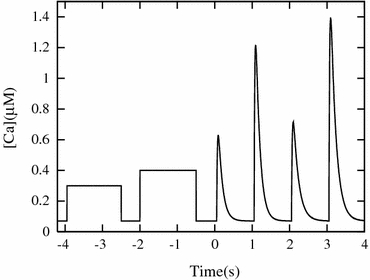
Ca-transients applied for the determination of ODE parameters. The last four were generated using the equation by Rice et al.20 with the parameter set listed in Appendix

Once the parameters \documentclass[12pt]{minimal} \usepackage{amsmath} \usepackage{wasysym} \usepackage{amsfonts} \usepackage{amssymb} \usepackage{amsbsy} \usepackage{mathrsfs} \usepackage{upgreek} \setlength{\oddsidemargin}{-69pt} \begin{document}$$ \left( {C\left( i \right)_{\xi ,\;\alpha ,\;\eta }^{\mu ,\beta ,\nu } } \right) $$\end{document} are determined, ODE simulations can be performed by approximating the combinatory probabilities in Eq. (19) by

\documentclass[12pt]{minimal} \usepackage{amsmath} \usepackage{wasysym} \usepackage{amsfonts} \usepackage{amssymb} \usepackage{amsbsy} \usepackage{mathrsfs} \usepackage{upgreek} \setlength{\oddsidemargin}{-69pt} \begin{document}$$ {}^{t}{\mathbf{p}}_{i}^{\xi ,\eta } \approx {}^{t}{\mathbf{W}}_{i} \left( {\xi ,\eta } \right) \cdot {}^{t}{\mathbf{p}}_{i} $$\end{document} 23

with

\documentclass[12pt]{minimal} \usepackage{amsmath} \usepackage{wasysym} \usepackage{amsfonts} \usepackage{amssymb} \usepackage{amsbsy} \usepackage{mathrsfs} \usepackage{upgreek} \setlength{\oddsidemargin}{-69pt} \begin{document}$$ {}^{t}{\mathbf{W}}_{i} \left({\xi,\eta } \right) = \left[\begin{array}{llll} {{}^{t}W\left({\xi,\;0{\text{N}},\;\eta,i}\right)} & 0 & 0 & 0 \\ 0 & {{}^{t}W\left({\xi,\;1{\text{N}},\;\eta,i} \right)} & 0 & 0 \\ 0 & 0 & {{}^{t}W\left({\xi,\;1{\text{P}},\;\eta,i} \right)} & 0 \\ 0 & 0 & 0 & {{}^{t}W\left({\xi,\;0{\text{P}},\;\eta,i} \right)} \\ \end{array} \right], $$\end{document} 24

where the diagonal entries are computed from

\documentclass[12pt]{minimal} \usepackage{amsmath} \usepackage{wasysym} \usepackage{amsfonts} \usepackage{amssymb} \usepackage{amsbsy} \usepackage{mathrsfs} \usepackage{upgreek} \setlength{\oddsidemargin}{-69pt} \begin{document}$$ {}^{t}W\left( {\xi ,\alpha ,\eta ,i} \right) = \exp \left( {\min \left( {0,\sum\limits_{{\mu ,\beta ,\nu = 0{\text{N}},1{\text{N}},1{\text{P}},0{\text{P}}}} {C\left( i \right)_{\xi ,\alpha ,\eta }^{\mu ,\beta ,\nu } {}^{t}\left\langle {\left[ \mu \right]\left[ \beta \right]\left[ \nu \right]} \right\rangle_{i} } } \right)} \right). $$\end{document} 25

Here, the minimum was applied so that ^t[ξ, α, η]_i ≤ ^t[α]_i is fulfilled in any case. Finally, by substituting \documentclass[12pt]{minimal} \usepackage{amsmath} \usepackage{wasysym} \usepackage{amsfonts} \usepackage{amssymb} \usepackage{amsbsy} \usepackage{mathrsfs} \usepackage{upgreek} \setlength{\oddsidemargin}{-69pt} \begin{document}$$ {}^{t}{\mathbf{p}}_{i}^{\xi ,\eta } $$\end{document} in Eq. (19) with the approximations in Eq. (23), we obtain an ODE:

\documentclass[12pt]{minimal} \usepackage{amsmath} \usepackage{wasysym} \usepackage{amsfonts} \usepackage{amssymb} \usepackage{amsbsy} \usepackage{mathrsfs} \usepackage{upgreek} \setlength{\oddsidemargin}{-69pt} \begin{document}$$ \frac{{d{}^{t}{\mathbf{p}}_{i} }}{dt} = \sum\limits_{{\xi ,\eta = {\text{N}},{\text{P}}}} {{}^{t}{\mathbf{A}}_{i} \left( {\xi ,\eta } \right) \cdot {}^{t}{\mathbf{W}}_{i} \left( {\xi ,\eta } \right) \cdot {}^{t}{\mathbf{p}}_{i} } \equiv {}^{t}{\mathbf{B}}_{i} \cdot {}^{t}{\mathbf{p}}_{i} ,\quad i = 1, \ldots ,nu, $$\end{document} 26

where the 4 × 4 matrix ^t B _i is given by

\documentclass[12pt]{minimal} \usepackage{amsmath} \usepackage{wasysym} \usepackage{amsfonts} \usepackage{amssymb} \usepackage{amsbsy} \usepackage{mathrsfs} \usepackage{upgreek} \setlength{\oddsidemargin}{-69pt} \begin{document}$$ {}^{t}{\mathbf{B}}_{i} = \sum\limits_{{\xi ,\eta = {\text{N}},{\text{P}}}} {{}^{t}{\mathbf{A}}_{i} \left( {\xi ,\eta } \right) \cdot {}^{t}{\mathbf{W}}_{i} \left( {\xi ,\eta } \right)} . $$\end{document} 27

The validity of this conceptual framework was supported by the excellent predictive power of the ODE model. Although there is no theoretical reason for adopting the exponential function in Eq. (21), we empirically found this style of function enhanced the approximation of temporal rate changes, especially for values close to zero.

Details of the determination and estimation of the ODE parameters are shown in the Appendix.

Interpolation of the ODE Parameters for the Simulations of Shortening Contraction

As previously shown, the parameters \documentclass[12pt]{minimal} \usepackage{amsmath} \usepackage{wasysym} \usepackage{amsfonts} \usepackage{amssymb} \usepackage{amsbsy} \usepackage{mathrsfs} \usepackage{upgreek} \setlength{\oddsidemargin}{-69pt} \begin{document}$$ C\left( i \right)_{\xi ,\;\alpha ,\;\eta }^{\mu ,\beta ,\nu } $$\end{document} can be estimated for individual MHs at a fixed SL. For the ODE simulation of shortening contraction where the SL is continuously changing, we adopted an interpolation method that uses the parameter values obtained at multiple SL’s {SL ₀, SL ₁,…,SL _NSL} with a constant interval ΔSL = SL _k − SL _k−1. Namely, for any SL between SL ₀ and SL _NSL:

\documentclass[12pt]{minimal} \usepackage{amsmath} \usepackage{wasysym} \usepackage{amsfonts} \usepackage{amssymb} \usepackage{amsbsy} \usepackage{mathrsfs} \usepackage{upgreek} \setlength{\oddsidemargin}{-69pt} \begin{document}$$ C\left( i \right)_{\xi ,\alpha ,\eta }^{\mu ,\beta ,\nu} = \left( {1 - \eta } \right)C\left( {SL_{k - 1} ,i} \right)_{\xi ,\alpha ,\eta }^{\mu ,\beta ,\nu } + \eta C\left( {SL_{k} ,i} \right)_{\xi ,\alpha ,\eta }^{\mu ,\beta ,\nu } \quad {\text{for}}\;SL_{k - 1} \le SL \le SL_{k} ,\;\;SL = \left( {1 - \eta } \right)SL_{k - 1} + \eta SL_{k} , $$\end{document} 28

In this study, ΔSL = 0.05 μm was adopted.

Computation

To reduce computational costs, the transition matrices ^t A _i(ξ, η) in Eq. (12) and ^t B _i in Eq. (27) (only for ODE) are updated only at 0.25 ms intervals, whereas the MC states and ODE solutions are updated at 2.5 μs intervals. Such a treatment significantly reduces the computational time for MC and ODE simulations without introducing recognizable error.

The MC and ODE simulation codes were written and executed using Fortran90 on a single core of Intel Xeon X7560 (2.27 GHz). The total number of MHs was 36. Using this previously described protocol, the computation of one sample of the MC simulation took 0.82 s per one second time length. To obtain reasonable mean values, more than a thousand MC samples were required. In contrast, an ODE that used the approximation given in Eqs. (19), (23) and (24) took 0.64 s per one second time length. Thus, the ODE model allowed a great reduction in computational time.

Results

Monte Carlo Simulation

In Fig. 4, the results from the MC simulations under steady-state condition are shown for force (in the following text, we use the fraction of bound cross-bridges [P](=[0P] + [1P]) as an index of developed force)–SL relations (Fig. 4a) and [P]–pCa relations (Fig. 4b). [P]–pCa relation clearly demonstrated a significant increase in the maximum Ca²⁺-activated force and increased Ca²⁺-sensitivity (a leftward shift of [Ca₅₀]) at longer SLs (see also Table 2), which is consistent with previous reports.5,14 The Hill coefficient decreased a little at short SLs, but its SL dependence was much smaller than that reported by Kentish et al.14 and closer to the recent results reported by Dobesh et al.5 (Fig. 4c). Data were not available for the shorter range of SLs in either of these experimental studies.

Figure 4.

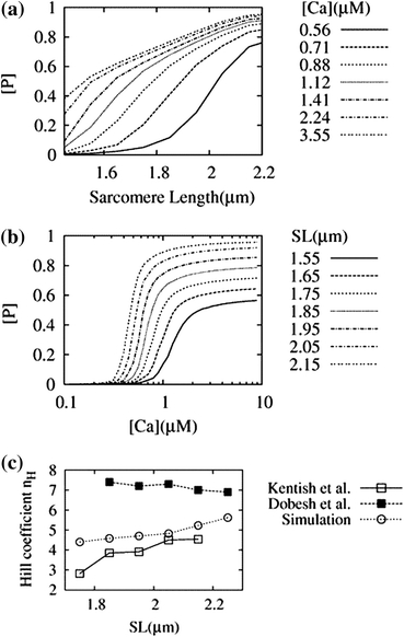
Results of MC simulation. Simulation was performed under constant Ca concentration and SL for 800 s (3.2 × 10⁸ steps). Data from the equilibrium phase (400–800 s) were averaged. The number of the P-state (0P + 1P) was assumed as the index of force. (a) Force–length (SL) relations shown for different Ca concentrations ranging from 0.56 to 3.55 μM. (b) [P]–pCa relations obtained for different SLs ranging from 1.45 to 2.15 μm. (c) SL dependence of the Hill coefficient. Simulation results (closed circle) were compared with the experimental results by Kentish et al.14 (open square) and Dobesh et al.5 (closed square)

Table 2.

Fitted Hill equation parameters for the MC simulation data

SL (μm)	[P]max	[Ca50] (μM)	Hill coefficient n H
1.55	0.567	1.40	3.96
1.65	0.645	1.12	4.29
1.75	0.716	0.94	4.40
1.85	0.787	0.81	4.58
1.95	0.856	0.70	4.70
2.05	0.920	0.61	4.82
2.15	0.957	0.53	5.23
2.25	0.967	0.50	5.62

Estimates of the ODE Parameters

The estimation of \documentclass[12pt]{minimal} \usepackage{amsmath} \usepackage{wasysym} \usepackage{amsfonts} \usepackage{amssymb} \usepackage{amsbsy} \usepackage{mathrsfs} \usepackage{upgreek} \setlength{\oddsidemargin}{-69pt} \begin{document}$$ \sum {C\left( i \right)_{\xi ,\;\alpha ,\;\eta }^{\mu ,\beta ,\nu } \;\;{}^{t}\left\langle {\left[ \mu \right]\left[ \beta \right]\left[ \nu \right]} \right\rangle_{i} } $$\end{document} in Eq. (22) was performed using the least square results of nu = 36 for each SL. MC simulation data were obtained from 10,000 samples for the Ca-transient that consists of the six peaks (Fig. 3). The results of this estimation analysis are shown for the units in the middle (MH₁₈) and near the filament edge (MH₅) at SL = 2.2 μm, in Fig. 5. Comparing the estimated values of \documentclass[12pt]{minimal} \usepackage{amsmath} \usepackage{wasysym} \usepackage{amsfonts} \usepackage{amssymb} \usepackage{amsbsy} \usepackage{mathrsfs} \usepackage{upgreek} \setlength{\oddsidemargin}{-69pt} \begin{document}$$ \left( {\sum {C\left( i \right)_{\xi ,\;\alpha ,\;\eta }^{\mu ,\beta ,\nu } \;\;{}^{t}\left\langle {\left[ \mu \right]\left[ \beta \right]\left[ \nu \right]} \right\rangle_{i} } } \right) $$\end{document} with the \documentclass[12pt]{minimal} \usepackage{amsmath} \usepackage{wasysym} \usepackage{amsfonts} \usepackage{amssymb} \usepackage{amsbsy} \usepackage{mathrsfs} \usepackage{upgreek} \setlength{\oddsidemargin}{-69pt} \begin{document}$$ \log \;\left( {{}^{t}[\xi ,\;\alpha ,\;\eta ]_{i} /{}^{t}[\alpha ]_{i} } \right) $$\end{document} (Eq. (22)) obtained from the MC simulations, fairly good approximations are attained overall, for all combinations of the indices and the units. However, we found variations that were dependent on the location of the units. For example, observing the unit located in the middle of the filament (MF₁₈), the plots for ξ, η = P, N and ξ, η = N, P in each of its states (0N, 1N, 1P, and 0P) (middle two rows of Fig. 5a) show similar patterns because of the unit’s symmetrical position along the filament, whereas the corresponding plots for the unit near the edge (MF₅) (middle two rows of Fig. 5b) show considerable differences. These findings indicate that the present estimation model is capable of capturing heterogeneous trends, which the models with the ring arrangement of the units3,19 cannot reproduce.

Figure 5.

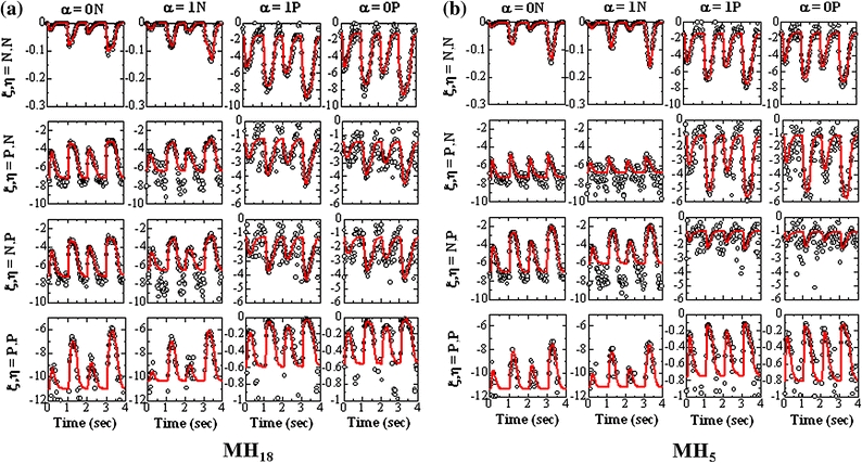
The least square fitting of the parameters. The values of \documentclass[12pt]{minimal} \usepackage{amsmath} \usepackage{wasysym} \usepackage{amsfonts} \usepackage{amssymb} \usepackage{amsbsy} \usepackage{mathrsfs} \usepackage{upgreek} \setlength{\oddsidemargin}{-69pt} \begin{document}$$ \sum {C(i)_{\xi ,\;\alpha ,\;\eta }^{\mu ,\beta ,\nu } \;{}^{IT}\langle {[ \mu ][ \beta][ \nu]} \rangle_{i} } $$\end{document} (red lines) estimated from the least square problem of Eq. (6) are compared with log W(ξ, α, η, i, IT) (circles), calculated from the MC simulation results using 10,000 samples for various combinations of the MH state (α, column) and the neighboring states (ξ and η, row). All results are from the MH₁₈ (the central unit in the filament) in the left panel and from MH₅ (near the left end of MF) in the right panel, respectively, for SL = 2.2 μm

Furthermore, wide variation is found in the values of log ^t W(ξ, α, η, i), supporting the use of a logarithmic scale when the close examination of ^t W(ξ, α, η, i) is required.

Comparing the ODE Model and MC Simulation Results

The ODE (Eq. (19)) was simulated using the approximations in Eqs. (23) and (24) to obtain the temporal changes of the fraction of bound cross-bridges [P] in response to the last four Ca peaks in Fig. 3, and the results were compared with those from the MC simulation at different SLs [1.9 and 2.2 μm (Fig. 6)]. In all MHs at both SLs, the ODE model and MC simulations correlated well. To clearly demonstrate the agreement, the absolute values of their differences were also shown (ERROR in Fig. 6).

Figure 6.

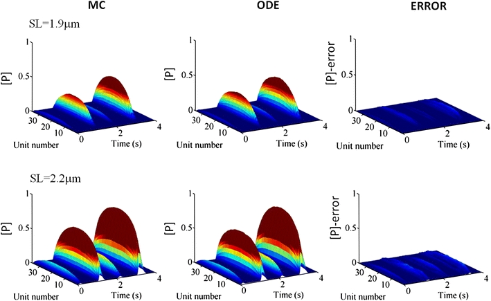
Comparisons between the ODE model and MC simulation at individual MHs. The fraction of bound cross-bridges [P] calculated using the ODE model (middle column) are compared with the MC simulation results (left column) while applying the Ca transients in Fig. 3. SL was set at 1.9 μm (top rows) or 2.2 μm (bottom rows). MC data are displayed as averaged values of 10,000 samples. The absolute values of the differences between the ODE and MC solutions are shown as ERROR (right column). The colors indicate the values (blue:0.0 red:0.3) of ratio (the fraction of bound cross-bridges [P]) (blue:0.0 red:0.3)

Effects of SL on Twitch Duration

Using the same parameter set, we simulated a series of isometric twitches using both the MC simulation and the ODE model while varying the SL and compared the time courses with the experimental results reported by Janssen et al.12 (Fig. 7). Because the Ca transient was not measured in Janssen’s study, we applied the Ca transient shown in the bottom panel, and the force and [P] values were normalized by their peak values at SL = 2.2 μm. Both the MC simulation (Fig. 7a) and the ODE model (Fig. 7b) reproduced the experimental results reasonably well and clearly showed the SL dependence of twitch duration.

Figure 7.

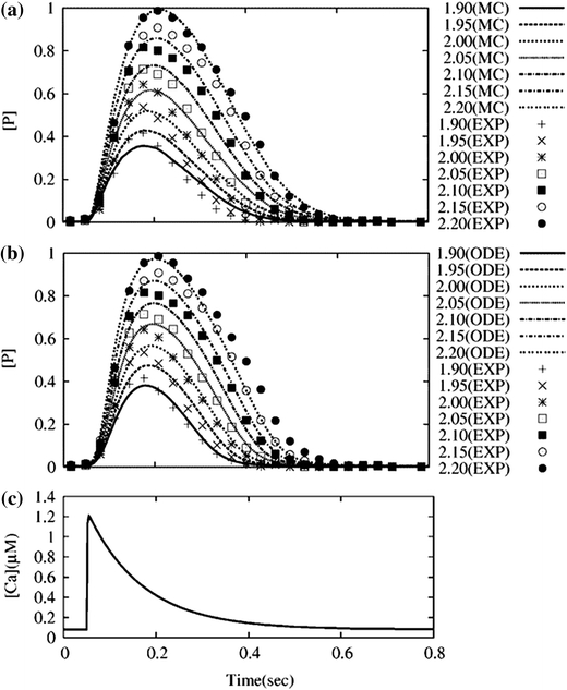
SL dependence of twitch durations. Isometric twitches were compared while varying the SL. (a) Comparisons between the experiment (symbols) and MC simulation (lines); (b) comparisons between the experiment (symbols) and ODE (lines); (c) applied Ca transient

Simulations of Isometric and Shortening Twitches

Next, we applied a Ca transient reported in Janssen and de Tombe11 to simulate a twitch under both isometric and shortening contraction (Fig. 8). Again we used the same parameter set, and the force and [P] values were normalized by the respective isometric peak values. For the simulation of a shortening twitch, we applied the time course of SL, and the interpolated parameter values were used for continuously changing SLs as described in the methods. Both the MC and ODE simulations successfully reproduced the experimental results (R ² = 0.987 for MC and R ² = 0.982 for ODE in the isometric contraction, and R ² = 0.988 for MC and R ² = 0.977 for ODE in the shortening contraction), however, to obtain the reasonable agreement, it was necessary to apply the Ca transient recorded under isometric condition to shortening twitch. The reason is not clear, but the use of [P] as the index of force and the absence of mechanisms regulating the affinity of Ca²⁺ to troponin C in the model may account for this contradictory result.

Figure 8.

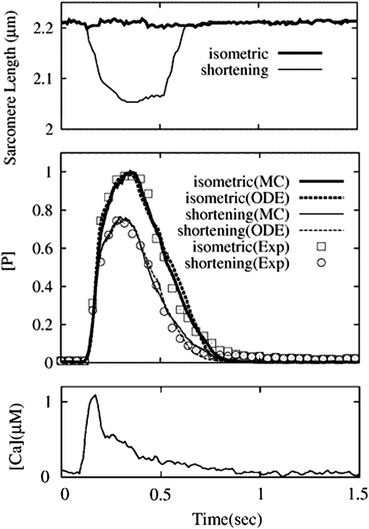
Model predictions of twitch contractions in response to experimentally observed Ca transient. Simulations were performed under isometric and shortening conditions. Ca transient (bottom panel) and length change (top panel) were digitized from the study by Janssen et al.11 Calculated force ([P] values) was compared for isometric (case 1) and shortening (case 2) among the MC simulation (solid lines), ODE (dotted lines), and experimental results (symbols). [P] and force were normalized relative to the peak isometric values

Effect of Cross-Bridge Kinetics on Force Relaxation

Finally, we examined the effect of cross-bridge kinetics on force relaxation by the MC and ODE simulations. For comparison, we adopted the results reported by Fitzsimons et al.7 in which a stepwise reduction in the Ca²⁺ concentration was applied to skinned rat trabeculae composed of either 80% α-myosin heavy chain (control) or 100% β-myosin heavy chain (hypothyroid). We used the same parameter set for control and reduced the rate constant (K_basic 10 to 3 in Eq. (5)) for the hypothyroid case to replicate the slow cycling rate of a β-myosin heavy chain. To obtain agreement between the MC and ODE simulations (R ² = 0.976), we used a memory length of 250 ms for the hypothyroid case. Both the MC and ODE simulations reproduced the exponential decline in [P] and the delay in force decline in the hypothyroid preparations that were observed in the experiment (Fig. 9). The half-times for relaxation (control vs. hypothyroid (ms)) were 80 and 152 (MC), and 72 and 117 (ODE) thus comparable to the experimental results (56 and 144) showing a 2-fold increase by hypothyroidism. Normalization of [P] by the initial value of the MC simulation made the initial ODE value greater than unity because of the differences in the numerical results between the two methods.

Figure 9.

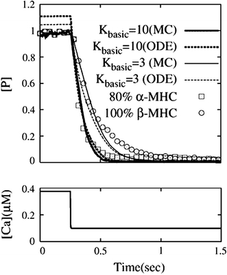
The effect of cross-bridge kinetics on the relaxation of force. We simulated experiments by Fitzsimons et al.,7 in which a step reduction in Ca²⁺ concentration (bottom panel) was applied to the skinned muscle preparations in which myosin isoform composition was either 80% α-myosin heavy chain or 100% β-myosin heavy chain. Top panel shows the comparison for 80% α(experiment: square, MC: thick solid line, ODE: thick dotted line) and 100% β(experiment: circle, MC: thin solid line, ODE: thin dotted line)

Discussion

In this study, we propose an ODE model of the cardiac sarcomere dynamics with which we can approximate the results of MC simulation performed on the spatially detailed sarcomere model. By this approach, we reduced the huge computational cost usually required for MC simulations. Very recently, Campbell et al.3 developed an ODE model similar to this model that describes nearest neighbor interactions. Their Markov model approach, without using approximation, theoretically gives us the accurate solution of the system, but the use of a ring configuration for the small number of regulatory units cannot reproduce the behavior of the units at the filament ends thus introducing errors. Additionally, the computational costs can become significant as the number of units approaches that of the actual thin filament. Furthermore, the ring simplification does not allow the simulation of SL change during the physiological contraction. Our ODE model with a realistic number of units in linear arrangement demonstrated good correlation with the MC simulation. Moreover, the results from our ODE model indicated that it can be applied to a wide range of cardiac physiology simulations.

Spatially-Detailed Sarcomere Model

The framework of the sarcomere model was adopted from the Ising model by Rice et al.19 with modifications. First, to fit the fraction of bound cross-bridges–pCa curves (Fig. 4 upper panel), modulatory factors for Ca binding (χ _RA) and cross-bridge formation (χ _RA · χ _LA) were multiplied by the transition rates. This modification also aided the reproducibility of the force–length relations.6,17 Importantly, it was confirmed that in different sets of data, the predictive power of the ODE model is independent of the factors χ _RA and χ _LA indicating that the ODE model could accommodate the modifications made to it.

Mean Field ODE vs. Spatially-Detailed Models

To avoid the expensive MC simulations required for spatially detailed models of the sarcomere, various ODE models describing the average behavior of the regulatory unit have been reported,13,15,20,21 but the problems and difficulties in the construction of such a mean field ODE model were pointed out in the literature.18 Because cooperativity involves the interactions among the spatially arranged molecules, heterogeneous responses of the units are naturally expected and, in fact, the MC simulation studies reported heterogeneous activities of the units during activation.10,22 Our MC simulation also revealed the heterogeneous activities of the units especially near the edge because these units lacking their neighbors on one side are destined to have small probability for making crossbridges. The smaller probability of these edge units in turn affects the kinetics of the adjacent units to reduce their probabilities. In this manner, the edge effect is transmitted to the center of the filament, although progressively attenuated, to create the symmetrical probability distribution as shown in Fig. 6. On the other hand, the probability distribution in this study (Fig. 6) is continuous thus making clear contrast to other spatial MC models, which show discrete “pockets” in probability distributions.2,10 This difference was originated by our assumption of homogeneous binding probability along the thin filament which ignores the discrete distribution of myosin binding site and differences in their interval (pitch) from that of MHs. With the inclusion of these structural properties, our ODE model will be able to provide detailed information on the activity of each unit and the overall sarcomere without the added computational cost, which an ordinary mean-field approach can never attain.

Memory Length

In the ODE simulations, we introduced the memory length as the parameter for the estimation of the combinatory probability of the states. As expected from Eq. (20), the memory length should be comparable to the lifetime of each state, which in turn reflects the cycling rate of cross-bridges. In fact, for the simulation of different myosins (Fig. 9), we needed to adjust the memory length. Such an adjustment is needed for myosins with different levels of light chain phosphorylation.

Application of the Model

We applied our model to the contraction simulation under a wide range of conditions and compared the results with experimental reports. Under steady-state conditions, [P]–pCa relations showed a weak dependence of the Hill coefficient on SL, which is close to recent data obtained under precise SL control. In response to the dynamic Ca transients, the model successfully reproduced the SL dependence of twitch duration under isometric conditions as well. However, the salient feature of the present model is its applicability to the shortening contraction. Although the present application was limited to the case of prescribed length change, the incorporation of a viscoelastic element to the model will enable us to simulate the dynamic experiment with a dynamically changing afterload.

Limitation

Our ODE approximation method is based on the assumption that the combinatory state probabilities of three consecutive MHs can be represented as functions of the state probabilities of single units, but does not have any firm theoretical basis. Yet, the good predictive power in the simulation tests provides strong support to the validity of the model. However, we cannot be sure whether we can obtain similar results under other conditions. Further studies are needed. Finally, to evaluate accurately the generated force in heart muscle contraction simulations, we must further introduce viscoelastic effects to the units in P-states.

Future Directions

The development of an ODE model that approximates a spatially detailed model may open the possibility of the application of such models to a large scale model of circulation, such as the finite element model of the heart. However, the theoretical basis of the present ODE approximation remains to be elucidated.

Appendix

Determination of the Parameters from MC Simulation Results

The data obtained from the MC simulations of duration [T ₀:T ₁] was divided into bins of equal time intervals (DT = 2.5 ms). Because updating in MC simulation was made every Δt = 2.5 μs, each bin was composed of 1000 data sets. In each updating step at each MH_i, the number of combinational states corresponding to (ξ _i−1, α _i, η _i+1) were counted, where ξ _i−1, η _i+1=N or P and α _i = 0N, 1N, 1P, or 0P. Results were stored in a 2 × 4 × 2 × nu × NT sized array cnt ₁₆(ξ _i−1, α _i, η _i+1, i, IT) for bin number IT = 1,…,NT(NT = T/DT) by using the following indexing: N = 1, P = 2 and 0N = 1, 1N = 2, 1P = 3, and 0P = 4. The above procedure was performed for the MC simulations repeated over 10,000 times for a single Ca condition (Fig. 3) to fill the array cnt ₁₆(ξ _i−1, α _i, η _i+1, i, IT). The following arrays (cnt ₄ and cnt ₂) were generated from this data holding the number of individual state of the MH_i in bin IT.

\documentclass[12pt]{minimal} \usepackage{amsmath} \usepackage{wasysym} \usepackage{amsfonts} \usepackage{amssymb} \usepackage{amsbsy} \usepackage{mathrsfs} \usepackage{upgreek} \setlength{\oddsidemargin}{-69pt} \begin{document}$$ \begin{aligned} cnt_{4} \left( {\alpha,i,IT} \right) &= \sum\limits_{{\xi,\eta = {\text{N}},{\text{P}}}} {cnt_{16} \left( {\xi,\alpha,\eta,i,IT} \right)} \hfill \\ cnt_{2} \left( {\mu,i,IT} \right) &= \left\{ \begin{array}{ll} {cnt_{4} \left({0{\text{N}},i,IT} \right) + cnt_{4} \left( {1{\text{N}},i,IT}\right),} & {\text{if} \; \mu = {\text{N}}} \\ {cnt_{4} \left({0{\text{P}},i,IT} \right) + cnt_{4} \left( {1{\text{P}},i,IT}\right),} & {\text{if} \; \mu = {\text{P}}} \\ \end{array} \right. \end{aligned} $$\end{document} A1

Dividing the elements of these two arrays by the total number of data provides the estimate of probability. Therefore, we can obtain the following ratio that approaches the left-hand side in Eq. (21) as the number of samples increases.

\documentclass[12pt]{minimal} \usepackage{amsmath} \usepackage{wasysym} \usepackage{amsfonts} \usepackage{amssymb} \usepackage{amsbsy} \usepackage{mathrsfs} \usepackage{upgreek} \setlength{\oddsidemargin}{-69pt} \begin{document}$$ W\left( {\xi ,\alpha ,\eta ,i,IT} \right) = \frac{{cnt_{16} \left( {\xi ,\alpha ,\eta ,i,IT} \right)}}{{cnt_{4} \left( {\alpha ,i,IT} \right)}} \approx \frac{{{}^{t}\left[ {\xi ,\alpha ,\eta } \right]_{i} }}{{{}^{t}\left[ \alpha \right]_{i} }}, $$\end{document} A2

for (IT − 1) · DT ≤ t ≤ IT · DT.

Approximations of \documentclass[12pt]{minimal} \usepackage{amsmath} \usepackage{wasysym} \usepackage{amsfonts} \usepackage{amssymb} \usepackage{amsbsy} \usepackage{mathrsfs} \usepackage{upgreek} \setlength{\oddsidemargin}{-69pt} \begin{document}$$ {}^{t}\left\langle {\left[ \mu \right]\left[ \beta \right]\left[ \nu \right]} \right\rangle_{i} $$\end{document} can also be obtained from cnt ₄ by applying the backward Euler time integration scheme to the ODE:

\documentclass[12pt]{minimal} \usepackage{amsmath} \usepackage{wasysym} \usepackage{amsfonts} \usepackage{amssymb} \usepackage{amsbsy} \usepackage{mathrsfs} \usepackage{upgreek} \setlength{\oddsidemargin}{-69pt} \begin{document}$$ \frac{d}{dt}{}^{t}\left\langle {\left[ \mu \right]\left[ \beta \right]\left[ \nu \right]} \right\rangle_{i} + \frac{1}{\tau }{}^{t}\left\langle {\left[ \mu \right]\left[ \beta \right]\left[ \nu \right]} \right\rangle_{i} = \frac{1}{\tau }{}^{t}\left[ \mu \right]_{i} {}^{t}\left[ \beta \right]_{i} {}^{t}\left[ \nu \right]_{i} ,T_{0} < t \le T_{1} $$\end{document} A3

that is fulfilled by \documentclass[12pt]{minimal} \usepackage{amsmath} \usepackage{wasysym} \usepackage{amsfonts} \usepackage{amssymb} \usepackage{amsbsy} \usepackage{mathrsfs} \usepackage{upgreek} \setlength{\oddsidemargin}{-69pt} \begin{document}$$ {}^{t}\left\langle {\left[ \mu \right]\left[ \beta \right]\left[ \nu \right]} \right\rangle_{i} $$\end{document} in Eq. (20) in the main text. This results in the following:

\documentclass[12pt]{minimal} \usepackage{amsmath} \usepackage{wasysym} \usepackage{amsfonts} \usepackage{amssymb} \usepackage{amsbsy} \usepackage{mathrsfs} \usepackage{upgreek} \setlength{\oddsidemargin}{-69pt} \begin{document} {}^{IT + 1}\left\langle {\left[ \mu \right]\left[ \beta \right]\left[ \nu \right]} \right\rangle = \frac{1}{DT + \tau }\left( {\tau \cdot {}^{IT}\left\langle {\left[ \mu \right]\left[ \beta \right]\left[ \nu \right]} \right\rangle\\ + DT \cdot \frac{mcnt(\mu ,\beta ,\nu ,i,IT)}{{\left( {DT/\Updelta t} \right)^{3} \cdot MT^{3} }}} \right)\\\;{\text{with}}\;mcnt(\mu ,\beta ,\nu ,i,IT) = cnt_{4} \left( {\mu ,i,IT} \right)cnt_{4}\\ \left( {\beta ,i,IT} \right)cnt_{4} \left( {\nu ,i,IT} \right).\end{document} A4

Here, MT is the repeat number of MC simulations, and the interval index IT is identified with time t = IT · DT − T ₀.

The parameters \documentclass[12pt]{minimal} \usepackage{amsmath} \usepackage{wasysym} \usepackage{amsfonts} \usepackage{amssymb} \usepackage{amsbsy} \usepackage{mathrsfs} \usepackage{upgreek} \setlength{\oddsidemargin}{-69pt} \begin{document}$$ C\left( i \right)_{\xi ,\;\alpha ,\;\eta }^{\mu ,\beta ,\nu } $$\end{document} were determined by minimizing the residual R in its logarithmic form as:

\documentclass[12pt]{minimal} \usepackage{amsmath} \usepackage{wasysym} \usepackage{amsfonts} \usepackage{amssymb} \usepackage{amsbsy} \usepackage{mathrsfs} \usepackage{upgreek} \setlength{\oddsidemargin}{-69pt} \begin{document}$$ R\left( {\xi ,\alpha ,\eta ,i,IT} \right) = \log \;W\left( {\xi ,\alpha ,\eta ,i,IT} \right) - \sum\limits_{{\mu ,\beta ,\nu = 0{\text{N}},1{\text{N}},1{\text{P}},0{\text{P}}}} {C\left( i \right)_{\xi ,\alpha ,\eta }^{\mu ,\beta ,\nu } {}^{IT}\left\langle {\left[ \mu \right]\left[ \beta \right]\left[ \nu \right]} \right\rangle } . $$\end{document} A5

In practice, we solved the following least-square problem for errors with weights of bias (cnt ₁₆) on the logW values derived from the larger number of samples assuming their reliability.

\documentclass[12pt]{minimal} \usepackage{amsmath} \usepackage{wasysym} \usepackage{amsfonts} \usepackage{amssymb} \usepackage{amsbsy} \usepackage{mathrsfs} \usepackage{upgreek} \setlength{\oddsidemargin}{-69pt} \begin{document}$$ E\left( {\xi ,\alpha ,\eta ,i} \right) = \sum\limits_{IT = 1}^{NT} {\frac{{cnt_{16} \left( {\xi ,\alpha ,\eta ,i,IT} \right)}}{MT}R\left( {\xi ,\alpha ,\eta ,i,IT} \right)^{2} + \varepsilon \sum\limits_{\mu ,\beta ,\nu } {\left( {C\left( i \right)_{\xi ,\;\alpha ,\;\eta }^{\mu ,\beta ,\nu } - \overline{C} } \right)^{2} } } $$\end{document} A6

Through this procedure, W = 0 is naturally eliminated in the error evaluation. The second term on the right-hand side of Eq. (A6) was added to avoid extraordinarily large values for the parameters \documentclass[12pt]{minimal} \usepackage{amsmath} \usepackage{wasysym} \usepackage{amsfonts} \usepackage{amssymb} \usepackage{amsbsy} \usepackage{mathrsfs} \usepackage{upgreek} \setlength{\oddsidemargin}{-69pt} \begin{document}$$ C\left( i \right)_{\xi ,\alpha ,\eta }^{\mu ,\beta ,\nu } . $$\end{document} In our simulations, ε = 10⁻⁵ and \documentclass[12pt]{minimal} \usepackage{amsmath} \usepackage{wasysym} \usepackage{amsfonts} \usepackage{amssymb} \usepackage{amsbsy} \usepackage{mathrsfs} \usepackage{upgreek} \setlength{\oddsidemargin}{-69pt} \begin{document}$$ \overline{C} = - 10 $$\end{document} were adopted.

The least square problem for the error E in Eq. (A6) results in the following system of linear equations with 64 unknowns \documentclass[12pt]{minimal} \usepackage{amsmath} \usepackage{wasysym} \usepackage{amsfonts} \usepackage{amssymb} \usepackage{amsbsy} \usepackage{mathrsfs} \usepackage{upgreek} \setlength{\oddsidemargin}{-69pt} \begin{document}$$ C\left( i \right)_{\xi ,\alpha ,\eta }^{{\bar{\mu },\bar{\beta },\bar{\nu }}} \;(\bar{\mu },\bar{\beta },\bar{\nu } = 0{\text{N}},1{\text{N}},1{\text{P}},0{\text{P}}). $$\end{document}

\documentclass[12pt]{minimal} \usepackage{amsmath} \usepackage{wasysym} \usepackage{amsfonts} \usepackage{amssymb} \usepackage{amsbsy} \usepackage{mathrsfs} \usepackage{upgreek} \setlength{\oddsidemargin}{-69pt} \begin{document}$$ \sum\limits_{{\bar{\mu },\bar{\beta },\bar{\nu }}} {\left( {a_{\mu ,\beta ,\nu }^{{\bar{\mu },\bar{\beta },\bar{\nu }}} + \varepsilon \;\;\delta_{\mu ,\beta ,\nu }^{{\bar{\mu },\bar{\beta },\bar{\nu }}} } \right)C\left( i \right)_{\xi ,\alpha ,\eta }^{{\bar{\mu },\bar{\beta },\bar{\nu }}} = b_{\mu ,\beta ,\nu } } ,\mu ,\beta ,\nu = 0{\text{N}},1{\text{N}},1{\text{P or }}0{\text{P}} $$\end{document} A7

Here, the coefficients in Eq. (A7) are given by

\documentclass[12pt]{minimal} \usepackage{amsmath} \usepackage{wasysym} \usepackage{amsfonts} \usepackage{amssymb} \usepackage{amsbsy} \usepackage{mathrsfs} \usepackage{upgreek} \setlength{\oddsidemargin}{-69pt} \begin{document}$$ \begin{aligned} a_{\mu,\beta,\nu }^{{\bar{\mu },\bar{\beta},\bar{\nu }}} &= \sum\limits_{IT = 1}^{NT} {\frac{{cnt_{16}\left( {\xi,\alpha,\eta,i,IT} \right)}}{MT}\;{}^{IT}\left\langle{\left[ \mu \right]\left[ \beta \right]\left[ \nu \right]}\right\rangle \;{}^{IT}\left\langle {\left[ {\bar{\mu }}\right]\left[ {\bar{\beta }} \right]\left[ {\bar{\nu }} \right]}\right\rangle } + \varepsilon, \hfill \\ b_{\mu,\beta,\nu } &=\sum\limits_{IT = 1}^{NT} {\frac{{cnt_{16} \left( {\xi,\alpha,\eta,i,IT} \right)}}{MT}\;{}^{IT}\left\langle {\left[ \mu \right]\left[ \beta \right]\left[ \nu \right]} \right\rangle \;\;\log \;W\left( {\xi,\alpha,\eta,i,IT} \right) - \varepsilon \left( {C\left( i \right)_{\xi,\;\alpha,\;\eta }^{\mu,\beta,\nu }- \overline{C} } \right)}, \hfill \\ \delta_{\mu,\beta,\nu}^{{\bar{\mu },\bar{\beta },\bar{\nu }}} &= \left\{\begin{array}{ll} {1,} & {{\text{if}} \; \bar{\mu } = \mu,\bar{\beta} = \beta,\bar{\nu } = \nu,} \\ {0,} & {{\text{otherwise}}.} \\ \end{array} \right. \end{aligned} $$\end{document} A8

Generation of test Ca transients

The last 4 Ca transients in Fig. 3 were generated by the following equation proposed by Rice et al.,20 with the parameter set listed below.

\documentclass[12pt]{minimal} \usepackage{amsmath} \usepackage{wasysym} \usepackage{amsfonts} \usepackage{amssymb} \usepackage{amsbsy} \usepackage{mathrsfs} \usepackage{upgreek} \setlength{\oddsidemargin}{-69pt} \begin{document}$$ \left[ {\text{Ca}} \right](t) = \left\{ \begin{array}{l}{\text{Ca}}_{\text{diastolic}} \\ \left({\frac{{{\text{Ca}}_{\text{amplitude}}\,-\,{\text{Ca}}_{\text{diastolic}} }}{\beta }} \right) \times \left({\exp \left( { - \frac{{t - t_{\text{start}} }}{{\tau_{1} }}}\right) - \exp \left( {\frac{{t - t_{\text{start}} }}{{\tau_{2}}}} \right)} \right) + {\text{Ca}}_{\text{diastolic}} \hfill \\ \end{array} \right. $$\end{document} A9

with

\documentclass[12pt]{minimal} \usepackage{amsmath} \usepackage{wasysym} \usepackage{amsfonts} \usepackage{amssymb} \usepackage{amsbsy} \usepackage{mathrsfs} \usepackage{upgreek} \setlength{\oddsidemargin}{-69pt} \begin{document}$$ \beta = \left( {\frac{{\tau_{1} }}{{\tau_{2} }}} \right)^{{ - 1/\left( {\frac{{\tau_{1} }}{{\tau_{2} }} - 1} \right)}} - \left( {\frac{{\tau_{1} }}{{\tau_{2} }}} \right)^{{ - 1/\left( {\frac{{\tau_{2} }}{{\tau_{1} }} - 1} \right)}} . $$\end{document} A10

\documentclass[12pt]{minimal} \usepackage{amsmath} \usepackage{wasysym} \usepackage{amsfonts} \usepackage{amssymb} \usepackage{amsbsy} \usepackage{mathrsfs} \usepackage{upgreek} \setlength{\oddsidemargin}{-69pt} \begin{document}$$ 1{\text{st:}}\;t_{\text{start}} = 0.05\,{\text{s}},\;{\text{Ca}}_{\text{diastolic}} = 0.07\,\mu {\text{M}},\;{\text{Ca}}_{\text{amplitude}} = 1.4\,\mu {\text{M}},\;\tau_{1} = 0.02\,{\text{s}},\;\tau_{2} = 0.11\,{\text{s}} $$\end{document}

\documentclass[12pt]{minimal} \usepackage{amsmath} \usepackage{wasysym} \usepackage{amsfonts} \usepackage{amssymb} \usepackage{amsbsy} \usepackage{mathrsfs} \usepackage{upgreek} \setlength{\oddsidemargin}{-69pt} \begin{document}$$ 2{\text{nd:}}\;t_{\text{start}} = 1.05\,{\text{s}},\;{\text{Ca}}_{\text{diastolic}} = 0.07\,\mu {\text{M}},\;{\text{Ca}}_{\text{amplitude}} = 2.8\,\mu {\text{M}},\;\tau_{1} = 0.02\,{\text{s}},\;\tau_{2} = 0.11\,{\text{s}} $$\end{document}

\documentclass[12pt]{minimal} \usepackage{amsmath} \usepackage{wasysym} \usepackage{amsfonts} \usepackage{amssymb} \usepackage{amsbsy} \usepackage{mathrsfs} \usepackage{upgreek} \setlength{\oddsidemargin}{-69pt} \begin{document}$$ 3{\text{rd:}}\;t_{\text{start}} = 2.05\,{\text{s}},\;{\text{Ca}}_{\text{diastolic}} = 0.07\,\mu {\text{M}},\;{\text{Ca}}_{\text{amplitude}} = 1.4\,\mu {\text{M}},\;\tau_{1} = 0.02\,{\text{s}},\;\tau_{2} = 0.14\,{\text{s}} $$\end{document}

\documentclass[12pt]{minimal} \usepackage{amsmath} \usepackage{wasysym} \usepackage{amsfonts} \usepackage{amssymb} \usepackage{amsbsy} \usepackage{mathrsfs} \usepackage{upgreek} \setlength{\oddsidemargin}{-69pt} \begin{document}$$ 4{\text{th:}}\;t_{\text{start}} = 3.05\,{\text{s}},\;{\text{Ca}}_{\text{diastolic}} = 0.07\,\mu {\text{M}},\;{\text{Ca}}_{\text{amplitude}} = 2.8\,\mu {\text{M}},\;\tau_{1} = 0.02\,{\text{s}},\;\tau_{2} = 0.14\,{\text{s}} $$\end{document}

References

- 1.Campbell K. Rate constant of muscle force redevelopment reflects cooperative activation as well as cross-bridge kinetics. Biophys. J. 1997;72:254–262. doi: 10.1016/S0006-3495(97)78664-8. [DOI] [PMC free article] [PubMed] [Google Scholar]
- 2.Campbell KS. Filament compliance effects can explain tension overshoots during force development. Biophys. J. 2006;91:4102–4109. doi: 10.1529/biophysj.106.087312. [DOI] [PMC free article] [PubMed] [Google Scholar]
- 3.Campbell SG, Lionetti FV, Campbell KS, McCulloch AD. Coupling of adjacent tropomyosins enhances cross-bridge-mediated cooperative activation in a Markov model of the cardiac thin filament. Biophys. J. 2010;98:2254–2264. doi: 10.1016/j.bpj.2010.02.010. [DOI] [PMC free article] [PubMed] [Google Scholar]
- 4.Daniel TL, Trimble AC, Chase PB. Compliant realignment of binding sites in muscle: transient behavior and mechanical tuning. Biophys. J. 1998;74:1611–1621. doi: 10.1016/S0006-3495(98)77875-0. [DOI] [PMC free article] [PubMed] [Google Scholar]
- 5.Dobesh DP, Konhilas JP, de Tombe PP. Cooperative activation in cardiac muscle: impact of sarcomere length. Am. J. Physiol. Heart Circ. Physiol. 2002;282:H1055–H1062. doi: 10.1152/ajpheart.00667.2001. [DOI] [PubMed] [Google Scholar]
- 6.Edman KA. Contractile properties of mouse single muscle fibers, a comparison with amphibian muscle fibers. J. Exp. Biol. 2005;208:1905–1913. doi: 10.1242/jeb.01573. [DOI] [PubMed] [Google Scholar]
- 7.Fitzsimons DP, Patel JR, Moss RL. Role of myosin heavy chain composition in kinetics of force development and relaxation in rat myocardium. J. Physiol. 1998;15:171–183. doi: 10.1111/j.1469-7793.1998.171by.x. [DOI] [PMC free article] [PubMed] [Google Scholar]
- 8.Geeves M, Griffiths H, Mijailovich S, Smith D. Cooperative [Ca2+]-dependent regulation of the rate of myosin binding to actin: solution data and the tropomyosin chain model. Biophys. J. 2011;100:2679–2687. doi: 10.1016/j.bpj.2011.04.020. [DOI] [PMC free article] [PubMed] [Google Scholar]
- 9.Hunter PJ, McCulloch AD, ter Keurs HEDJ. Modeling the mechanical properties of cardiac muscle. Prog. Biophys. Mol. Biol. 1998;69:289–331. doi: 10.1016/S0079-6107(98)00013-3. [DOI] [PubMed] [Google Scholar]
- 10.Hussan J, de Tombe PP, Rice JJ. A spatially detailed myofilament model as a basis for large-scale biological simulations. IBM J. Res. Dev. 2006;50:583–600. doi: 10.1147/rd.506.0583. [DOI] [Google Scholar]
- 11.Janssen PM, de Tombe PP. Uncontrolled sarcomere shortening increases intracellular Ca2+ transient in rat cardiac trabeculae. Am. J. Physiol. 1997;272:H1892–H1897. doi: 10.1152/ajpheart.1997.272.4.H1892. [DOI] [PubMed] [Google Scholar]
- 12.Janssen PM, Hunter WC. Force, not sarcomere length, correlates with prolongation of isosarcometric contraction. Am. J. Physiol. 1995;269:H676–H685. doi: 10.1152/ajpheart.1995.269.2.H676. [DOI] [PubMed] [Google Scholar]
- 13.Katsnelson LB, Sulman TB, Solovyova OE, Markhasin VS. Cooperative mechanisms of thin filament activation and their contribution to the myocardial contractile function: assessment in a mathematical model. Biophysics. 2009;54:39–46. doi: 10.1134/S0006350909010072. [DOI] [PubMed] [Google Scholar]
- 14.Kentish JC, ter Keurs HEDJ, Ricciardi L, Bucx JJJ, Noble MIM. Comparison between the sarcomere length–force relations of intact and skinned trabeculae from rat right ventricle: influence of calcium concentrations on these relations. Circ. Res. 1986;58:755–768. doi: 10.1161/01.res.58.6.755. [DOI] [PubMed] [Google Scholar]
- 15.Landesberg A, Sideman S. Mechanical regulation of cardiac muscle by coupling calcium kinetics with cross-bridge cycling. Am. J. Physiol. 1994;267:H779–H795. doi: 10.1152/ajpheart.1994.267.2.H779. [DOI] [PubMed] [Google Scholar]
- 16.Mijailovich SM, Fredberg JJ, Butler JP. On the theory of muscle contraction: filament extensibility and the development of isometric force and stiffness. Biophys. J. 1996;71:1475–1484. doi: 10.1016/S0006-3495(96)79348-7. [DOI] [PMC free article] [PubMed] [Google Scholar]
- 17.Rassier DE, Macintosh BR, Herzog W. Length dependence of active force production in skeletal muscle. J. Appl. Physiol. 1999;86:1445–1457. doi: 10.1152/jappl.1999.86.5.1445. [DOI] [PubMed] [Google Scholar]
- 18.Rice JJ, de Tombe PP. Approaches to modeling cross-bridges and calcium-dependent activation in cardiac muscle. Prog. Biophys. Mol. Biol. 2004;85:179–195. doi: 10.1016/j.pbiomolbio.2004.01.011. [DOI] [PubMed] [Google Scholar]
- 19.Rice JJ, Stolovitzky G, Tu Y, de Tombe PP. Ising model of cardiac thin filament activation with nearest-neighbor cooperative interactions. Biophys. J. 2003;84:897–909. doi: 10.1016/S0006-3495(03)74907-8. [DOI] [PMC free article] [PubMed] [Google Scholar]
- 20.Rice JJ, Wang F, Bers DM, de Tombe PP. Approximate model of cooperative activation and crossbridge cycling in cardiac muscle using ordinary differential equations. Biophys. J. 2008;95:2368–2390. doi: 10.1529/biophysj.107.119487. [DOI] [PMC free article] [PubMed] [Google Scholar]
- 21.Rice JJ, Winslow RL, Hunter WC. Comparison of putative cooperative mechanisms in cardiac muscle: length dependence and dynamic responses. Am. J. Physiol. Heart Circ. Physiol. 1999;276:1734–1754. doi: 10.1152/ajpheart.1999.276.5.H1734. [DOI] [PubMed] [Google Scholar]
- 22.Zou G, Phillips GN., Jr A cellular automaton model for the regulatory behavior of muscle thin filaments. Biophys. J. 1994;67:11–28. doi: 10.1016/S0006-3495(94)80475-8. [DOI] [PMC free article] [PubMed] [Google Scholar]