Finger tapping movements of Parkinson’s disease patients automatically rated using nonlinear delay differential equations

Abstract

Parkinson’s disease is a degenerative condition whose severity is assessed by clinical observations of motor behaviors. These are performed by a neurological specialist through subjective ratings of a variety of movements including 10-s bouts of repetitive finger-tapping movements. We present here an algorithmic rating of these movements which may be beneficial for uniformly assessing the progression of the disease. Finger-tapping movements were digitally recorded from Parkinson’s patients and controls, obtaining one time series for every 10 s bout. A nonlinear delay differential equation, whose structure was selected using a genetic algorithm, was fitted to each time series and its coefficients were used as a six-dimensional numerical descriptor. The algorithm was applied to time-series from two different groups of Parkinson’s patients and controls. The algorithmic scores compared favorably with the unified Parkinson’s disease rating scale scores, at least when the latter adequately matched with ratings from the Hoehn and Yahr scale. Moreover, when the two sets of mean scores for all patients are compared, there is a strong (r = 0.785) and significant ($p<0.0015$) correlation between them.

Parkinson’s disease (PD) is a common disease affecting tens of millions of people worldwide. Its cardinal signs are resting tremor, bradykinesia (slowness clumsiness of movement), rigidity, and loss of postural reflexes. The disease evolves slowly and, to adjust medications to the severity of the disease, there is a need for automatic and objective evaluation of movements. Such objective movement assessments would supplement subjective clinical ratings, which are ordinal rather than metric and often show large inter-rater variability. Rather than using a spectral based technique, we rated dynamical features of each individuals’ finger-tapping—one of the items from the unified Parkinson’s disease rating scale (UPDRS) used for rating the severity of the disease—by using data models based on nonlinear delay differential equations (DDEs). The coefficients of the DDEs are then used to assess the severity of the disease.

INTRODUCTION

PD is a chronic neurodegenerative disease whose primary pathophysiology is loss of the dopamine containing cells in the basal ganglia.¹ Deprived of their normal dopaminergic inputs, nuclei within the basal ganglia become dysfunctional leading to abnormal neural oscillations and synchronization within multiple basal ganglia-cortical circuits.² These circuit disturbances lead to the clinical manifestations of the disease, which include such motor impairments as bradykinesia (slow movements), muscle rigidity, resting tremor, and postural instability. The impairment in voluntary movement in PD is characterized by a number of specific sensorimotor processing deficits, including a generalized slowness of movement;³ a difficulty in carrying out sequential movements;⁴ a reliance on sensory input, particularly visual input, to guide and correct movement;^{5, 6} and difficulties in timing, synchronizing, and coordinating movements.^{7, 8, 9}

Since Parkinson’s disease is a degenerative disease, an effective tool is needed to track changes in its severity and the effectiveness of remedial treatments. Clinical evaluations can be costly and difficult to execute consistently over the long duration of the disease. The first rating scale—the Hoehn and Yahr (HY) scale¹⁰—was designed originally to be a simple descriptive scale for providing a general estimate of clinical function, combining functional deficits and objective signs. 0.5 increments were later introduced.¹¹ The original HY scale is as follows:

• (1)Unilateral involvement only usually with minimal or no functional disability;
• (2)Bilateral or midline involvement without impairment of balance;
• (3)Bilateral disease: mild to moderate disability with impaired postural reflexes; physically independent;
• (4)Severely disabling disease; still able to walk or stand unassisted; and
• (5)Confinement to bed or wheelchair unless aided.

As in any clinical rating scale, subjective measures are used in the HY scale and thus may vary among physicians. Consequently, another rating scale—the UPDRS—was introduced later¹² to overcome the inter-rater variability and to provide a more fine-grained assessment of motor dysfunction (see Ref. 11 for a review about limitations in the use of HY scale). The UPDRS is a rating tool to characterize PD severity and to follow the evolution of the disease.¹³ It is comprised of four sections: (1) mentation, behavior, and mood, (2) activity of daily living (ADL), (3) motor function, and (4) complications of therapy, totaling 45 items. Each item is evaluated by interview, or for motor function, by visual scoring of specific movements and by passive manipulation of the joints. The most commonly used section of the UPDRS is the motor section, since motor dysfunction has been the core defining clinical feature of the disease. The UPDRS motor section has a maximum score of 108 points representing the worst (total) disability and 0 corresponding to no disability.

One of the most important characteristics of impaired movement in PD is bradykinesia, a broad term encompassing slow, clumsy movements. Bradykinesia is widely tested for in the motor section of the UPDRS. There are three tests of arm and hand movements, all involving sequential movements, which reliably evaluate bradykinesia. These three tests are finger-to-thumb tapping (item 23), hand opening and closing (item 24), and hand pronation and supination (item 25). Finger tapping correlates better with the overall UPDRS clinical scores than items 24 or 25 (Ref. ²⁷). Moreover, the motor performance of PD patients degrades with task completion far more easily during sequential opposition of individual finger movements than during non-individual finger oppositions.²⁸ The dynamics underlying movements of PD patients was, therefore, investigated by recording 10 s bouts of individual finger tapping movements. These movements were repetitive index-thumb oppositions, instructed to be of large constant amplitude, produced smoothly and rapidly.

While the UPDRS provides an improved instrument for rating PD motor severity compared to the HY scale and has overall better clinimetric properties than other scales,¹⁴ it does not completely overcome the issues of inter-rater variability and subjectivity^{15, 16} and remains a time consuming rating technique. Hence, although it is the most studied and used scale, it cannot be applied as often as desired to track the progression of the disease.

Consequently, there is a need for automatic, graded measurements of Parkinsonian motor dynamics that are metric rather than ordinal. For this purpose, commercial accelerometer and gyroscope sensors are often used (see for instance Ref. 17). The time series these generate have been analyzed using spectral analysis¹⁸ or adaptive Fourier modeling.¹⁹

However, spectral analysis has serious limitations when applied to short time series. The 10 s sessions recommended for evaluating patients²⁰ provide about 30 or 40 oscillations, which are not enough for an accurate spectral analysis of the underlying dynamics. To overcome these limitations, we propose an alternative technique based on non-linear modeling that is known to be efficient even when applied to short time series.^{21, 22, 23} A global modeling technique extracts from a time series a set of difference or differential equations whose iteration or integration reproduces the dynamics underlying the measurements. To enlarge the domain of applicability of this technique, we do not look for global models, but rather for a rough approximation of the underlying dynamics by using delay differential equations, which are known to provide good classifiers.^{24, 25, 26}

In the present study, PD motor dysfunction, made apparent by abnormal or dysfunctional finger-tapping dynamics, was assessed using rough approximations of the underlying dynamics using delay differential equations (DDE) (Refs. ^{24, 25, 26}). DDEs are known to be very flexible, that is, to capture a wide variety of dynamics with few terms. Moreover, DDEs are robust against noise contamination. The coefficient space associated with these DDEs was used to provide a measure of PD severity. These results then were compared to those obtained using the UPDRS to rate the quality of the finger tapping movements.

The remainder of this paper is organized as follows. Section 2 describes the patients and the protocol for recording the finger tapping movements. Section 3 discusses dynamical analysis of the data using a few tools borrowed from nonlinear dynamical systems theory and shows that these cannot discriminate PD patients from control subjects. Section 4 is devoted to the classification of PD patients and control subjects using optimized coefficients of a selected DDE. We then compare these results to the UPDRS tapping ratings. Section 5 provides some conclusions and perspectives.

PATIENTS AND MEASUREMENTS

Thirteen PD patients, together with thirteen controls, selected so that their ages were in approximate 1-1 correspondence with patients’ ages, were enrolled in our protocol after signing the informed consent document approved by the human subjects ethics committee of the University of California at San Diego. We began this study with data from the first six patients and controls, who we refer to as group i. The next seven PD patients and controls were enrolled later as part of a different study and are referred to here as group ii. There is a slight difference in data acquisition, detailed below.

All patients were studied “off-medication,” as defined in Ref. 20, using the same operational criteria of having not taken their anti-parkinsonian medications for at least 12 h prior to testing; all patients were tested at the same time during the day (in the morning); and the same 12 camera 3D optoelectronic camera system was used (see below). The 3D movement tracking system was quite precise—each camera has an optical resolution of $3600\times 3600$ (12 megapixels) using two linear detectors with 16-bit dynamic range and has an onboard processor that produces a subpixel resolution of $30000\times 30000$. Given the precision of the movement recordings and the nature of the human movements being recorded, a sampling frequency of 120 Hz, as well as that of 480 Hz, was deemed sufficient.

The clinical severity of the 13 PD patients at the time of testing was rated according to item 23 (finger tapping) of the UPDRS using the rules as follows:¹³

• 0 = Normal;

• 1 = Mild slowing and/or reduction in amplitude;

• 2 = Moderately impaired. Definite and early fatiguing. May have occasional arrests in movement;

• 3 = Severely impaired. Frequent hesitation in initiating movements or arrests in ongoing movement; and

• 4 = Can barely perform the task.

All clinical severity ratings were given by the same person.

Item 23 counts for 4 points out of a total of 108 for the entire UPDRS motor score and correlates well with the overall motor score. Also, PD patients were given an overall severity rating according to the HY scale (Table TABLE I.) as recommended.²⁰ They ranged from mild (2) to moderately (3) impaired.

TABLE I.

Clinical characteristics of Parkinson’s disease patients for the two groups.

Group	PD patient number	Age (years)	Sex	Handedness	Disease duration (years)	HY score	UPDRS score	Medications a
i	1	66	M	R	7	2	1.0, 1.0, 1.5, 2.0	Sel, Lev, Br
	2	75	M	L	8	2	0.5	Br, Ras
	3	75	M	R	6	3	3.0, 3.0	St
	4	49	M	R	8	3	3.0, 3.0, 3.0	Lev, LevR, Sel, Ent, Rot
	5	73	M	R	8	2	1.5, 2.0, 2.5	Lev, Pr, Sel, Am
	6	76	M	R	5	2	2.0, 2.0, 2.0	Lev, Pr, Am
ii	7	71	M	R	12	2	1.0, 2.0, 3.0	St, Rop, Sel
	8	67	M	R	9	2	2.0, 1.5, 2.5	Lev, Ent, Art
	9	68	F	R	11	3	1.0, 1.0, 1.5	Lev, Pr, Ent
	10	62	F	R	9	2	1.5, 1.5, 2.0	Lev, Pr
	11	66	F	R	9	2	2.0, 1.5, 1.0	Pr, Sel, Am
	12	70	M	R	24	3	1.5	LevR, Ent, Pr, Am, Sel
	13	67	M	L	8	3	2.0	Lev, Pr, St

^aMedication codes: Am, Amantadine; Art, Artane (trihexyphenidyl); Br, Bromocriptine; Ent, Entacapone; Lev, Carbidopa/levodopa (regular formulation); LevR, Carbidopa/levodopa sustained release; Pr, Pramipexole; Ras, Rasagiline; Rop, Ropinirole; Rot, Rotigotine; Sel, Selegiline; and St, Stalevo (Carbidopa/levodopa/entacapone).

All subjects—both PD patients and controls—were asked to tap the index finger and thumb together making large, smooth, rapid movements for 10 s, spaced apart by 1 min. Subjects had their eyes open throughout.

To track finger movements, the subjects’ index fingertip and thumb were fitted with light-weight infrared emitting diodes (IREDs) approximately 5 mm in diameter. Our active marker 3D motion capture system (PhaseSpace, Inc., San Leandro, CA) consisted of twelve cameras placed in a semi-circle 1-2.5 m from the subject, who was seated at a table. We calibrated the system prior to each data collection. We checked that placement of the IRED markers did not perturb the motion of the digits in the following manner. The markers were taped to the index fingernail and to the nail of the thumb, and visually inspected to make sure that no part of a marker was in contact with the digital interphalangeal joint of either digit. This left all joints of the hand free to move. Subjects were then asked to fully flex and extent the fingers of their hand. The movements were visually inspected to make sure that there was no restriction in the motion, and subjects were asked if they felt any restriction. No restriction of perturbations of the finger movements were observed or reported. The data may have occlusion artifacts which occur when fewer than two cameras detect either of the IRED markers.

The data acquisition protocol for groups i and ii was almost identical,²⁹ but differed in sampling frequency—120 Hz for group i and 480 Hz for group ii—and in camera placement. The ratio of mild to moderate patient impairment was roughly the same for both groups.

Three 10 s sessions of individual finger tapping by the dominant hand were recorded for group i subjects and six sessions, three for each hand, for group ii subjects. The rates of recorded occlusions, defined as 100* (number of occluded data points)/(total number of data points), are reported in Table TABLE II.. When occlusions are present in a data set, the data analysis procedure, described below, causes more data points to be removed, thus raising the rate of effective occlusions.

TABLE II.

Rate of recorded occlusions for the data of both groups.

Group	Control subjects (%)	PD patients (%)
i	16.1	5.9
ii	3.5	3.8

The two groups of patients are characterized by a similar mean age, ($69\pm 10$) years for group i and ($67\pm 3$) years for group ii, but the disease duration was significantly different ($p<0.01$) (mean duration was ($7.0\pm 1.3$) years for group i and ($11.7\pm 5.6$) years for group ii). Importantly, the mean UPDRS finger tapping ratings were 24% higher for group i ($2.1\pm 0.8$) than for group ii ($1.7\pm 0.4$), reflecting a greater severity of motor impairment. However, this difference just failed to reach statistical significance $p\approx 0.087$. These statistics are summarized in Table TABLE III.. All p-values reported in this paper are computed from a Wilcoxon T-test.

TABLE III.

Statistics for age, disease duration, and UPDRS finger-tapping score.

	Average			SD
	Age	Duration	UPDRS	Age	Duration	UPDRS
Group i	69	7.0	2.1	10	1.3	0.8
Group ii	67	11.7	1.7	3	5.6	0.4

Note that group i patients had a larger standard deviation for their age and UPDRS finger-tapping score, but had a smaller standard deviation for disease duration. In other words, group i was less homogeneous than group ii in their age and UPDRS finger-tapping scores. Since Parkinson’s disease always progresses with age (i.e., UPDRS scores increase), one expects to see a correlation between variance in age and variance in UPDRS score. Table TABLE III., columns 4 and 6, is consistent with this observation. Although PD patients in both groups had typical, idiopathic Parkinson’s disease, and all were in Hoehn and Yahr stage 2 or 3 of the disease, patients in group i exhibited greater severity of motor dysfunction on the UPDRS rating of finger tapping. Having groups differing in motor severity, even within the same overall stage of the disease, allow us to examine our method across a wider range of motor deficits in PD patients who are clinically typical, and without the cognitive and emotional decline that occurs in more advanced stages of the disease.

We use the data without any preprocessing (not even the filtering above 10 Hz commonly used when human motions are investigated), since preprocessing such as filtering or smoothing could change some dynamical information in the data. One or more recorded occlusions give rise to several more effective occlusions after derivatives have been taken and a particular nonlinear DDE model applied. The rate of effective occlusions depends on the model used.

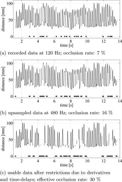
So that the same DDEs could be used on the data from both groups, all the time series of group i were upsampled to 480 Hz using the matlab routine “resample.” This upsampling increased the rate of effective occlusions: in each data set, the first and last 10 data points of each continuous data segment had to be removed due to the ambiguity of upsampled data at the beginning or end of a data segment. Therefore, a time series with one big occlusion has fewer points removed than the same time series with a lot of small occlusions since each continuous data segment loses 20 data points in this procedure. Fig. 1a presents the time series of the raw distances between the thumb and index finger for a subject in group i, whose movements were recorded at 120Hz. This trial had 7% occluded data points in the original, raw, data recording. Fig. 1b presents the occlusions after the data have been upsampled to 480 Hz, and Fig. 1c shows the effective occlusions.

Figure 1.

(Color online) Distance between thumb and index finger markers are plotted over time. Example of a time series with 7% occlusions in the recorded data (a). The dots denote the occluded points. The upsampled data (b) have an occlusion rate of 16%. In (c) after removing all effective occlusions, 70% of the original data is usable.

The effective occlusions depend on the computation of derivatives and on the structure of the DDE model being used. Depending on the window size used to compute the derivative, data points at both ends of a contiguous segment of data have to be removed. Finally, consider that the DDE models used in this paper relate data points at time t to data points at delayed times $t-{\tau }_j,$ with j = 1, 2, 3. The data point at time t is removed and effectively occluded if the derivative cannot be computed or the necessary delayed data points do not exist. If the effective occlusion rate was more than 50% of the time series, the time series was discarded. In dataset i, 13 out of 34 datafiles had effective occlusion rates greater than 50% and hence were rejected, and in dataset ii, no files had effective occlusion rates greater than 50%.

The majority of data files (81%) had no occlusions whatsoever. For those trials in which occlusions did occur, the small sections of the time series corresponding to the missing data were simply left blank.

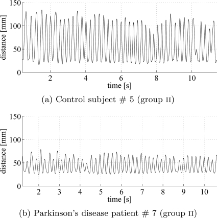
The distance between index finger and thumb was computed at each time step from the raw data files containing the xyz-coordinates of the finger and thumb IREDs. Typical time series are shown for a control subject (Fig. 2a) and a PD patient (Fig. 2b) from group ii. The cycle time for PD patients was generally around 200 ms. Both controls and PDs show variability in the amplitude of finger tapping.

Figure 2.

Time series of the distance between the thumb and the index finger during the individual finger tapping for a control subject (a) and a PD patient (b) from group ii. The sampling rate equals to 480 Hz. Note, that the PD patient has much reduced movement amplitude. However, there was substantial overlap in movement amplitude between the control subjects and PD patients and amplitude alone was not sufficient to discriminate the groups.

DYNAMICAL ANALYSIS

Fig. 2 suggests that finger-tap amplitude might distinguish between controls and PD patients. To evaluate whether there is significant difference in the statistics of the finger-tapping amplitude $A_n$—the difference between the maximum and the minimum of the distance for the nth tap—we computed the amplitude of each finger tap for all sessions for every subject. The standard deviation ${\sigma }_A$ is slightly less for the control subjects (${\overline{\sigma }}_A=0.22\pm 0.09$) than for the PD patients (${\overline{\sigma }}_A=0.26\pm 0.07$), but not significantly so ($p=0.1>0.05$). Therefore, fluctuations in the finger tapping amplitude cannot be used to discriminate between control subjects and PD patients.

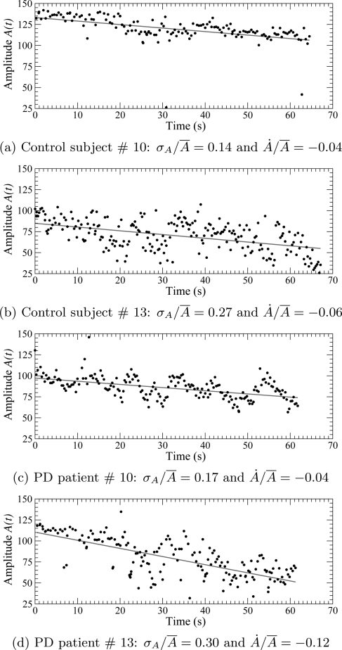
When the six 10 s sessions are concatenated in the order of recording, from the first to the last, there is a general tendency for a reduction in the finger tapping amplitude (Fig. 3). Could the difference in rates of reduction distinguish between controls and PD patients? Using the slope of the regression line ($\dot{A}$) normalized by the mean amplitude ($\overline{A}$), we find $\dot{A}/\overline{A}=-0.03\pm 0.05$ in control subjects and $\dot{A}/\overline{A}=-0.08\pm 0.05$ in PD patients. Once again, these differences are not significant ($p\approx 0.2>0.05$). In both groups, small as well as large amplitude fluctuations can be observed. This confirms the well known fact that there is significant variability across different instances of producing a given movement pattern, shown by control subjects as well as by patients. It is, therefore, necessary to use tools borrowed from nonlinear dynamical systems theory to investigate the dynamics underlying finger tapping.

Figure 3.

(Color online) Amplitude versus time for individual finger tapping by control subjects—(a) and (b)—and by PD patients—(c) and (d)—from group ii. The six 10 s sessions are concatenated to exhibit the tendency. Linear regression is shown as a red line. $\stackrel{·}{A}$ is the slope of the regression line and $\overline{A}$ is the mean amplitude.

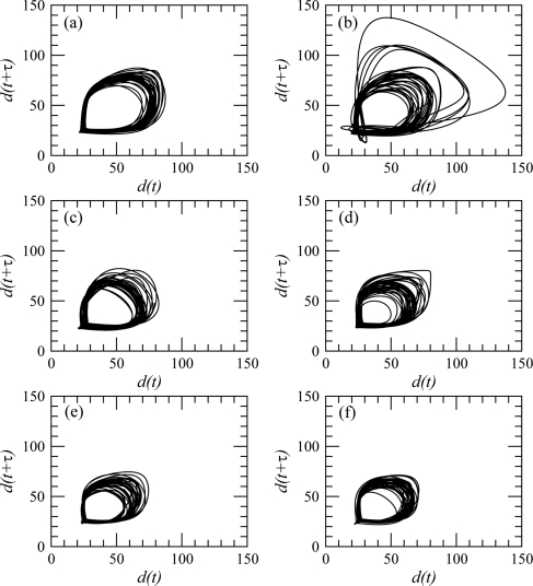
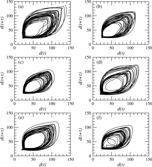
One of the very first steps of a dynamical analysis is to reconstruct a phase portrait from measurements using delay or derivative coordinates.³⁰ Delay coordinates are here used with a delay ${\tau }_r$ equal to $25\delta t$ where $\delta t=\frac{1}{480}$ s, that is, to a value around a quarter of the pseudo-period of the observed oscillations.^{31, 32} Typical phase portraits are shown for a control subject (Fig. 4) and a PD patient (Fig. 5), respectively. Six phase portraits are shown for each subject, one for each 10 s session. In both cases, the tendency of the finger tapping amplitude to decrease with time is recovered, since the diameter of the phase portrait is larger during the first sessions (Figs. 4a and 5a) than during the last ones (Figs. 4f and 5f).

Figure 4.

Phase portrait reconstructed from the distance between the index finger and the thumb using the delay coordinates. Case of control subject no. 13 (group ii).

Figure 5.

Phase portrait reconstructed from the distance between the index finger and the thumb using the delay coordinates. Case of PD patient no. 8 from group ii.

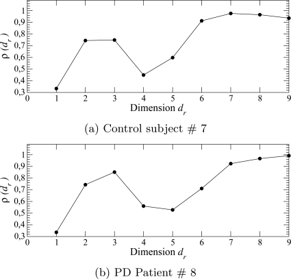
These phase portraits reveal a highly structured dynamics, that is, in any neighborhood of the phase portraits, trajectories are mainly governed by a unique vector field since they are locally parallel. This feature suggests a low-dimensional underlying dynamics. To check this, an embedding dimension was estimated using a false nearest neighbors algorithm.³³ The rate of true nearest neighbors evolves in similar ways for control subjects (Fig. 6a) and PD patients (Fig. 6b). The curves do not saturate for a dimension less than 6 (control subjects) or 7 (PD patients). Once again, it is rather difficult to discriminate control subjects from PD patients.

Figure 6.

Estimating the embedding dimension using a false nearest neighbors technique. Case of a control subject (a) and a PD patient from group ii. The fourth finger tapping session was here used.

The evolution of the rate of true nearest neighbors versus the dimension of the reconstructed phase portrait in Fig. 6 is similar to the one observed when the Rössler attractor is reconstructed from the third variable, z, in the Rössler equations (see Fig. 6 in Ref. 34). The rate of true neighbours decreases after a first maximum when the dimension used for reconstructing the phase space is equal to three. Such an oscillation of the rate of true neighbours was also observed when variable z of the Rössler system was used in the reconstruction procedure. In both cases, the reconstructed phase portrait presents a zone, known as a lethargy, where each revolution is not well distinguished from the others. Consequently, due to limited measurement accuracy, it is no longer possible to have different pre-images for every pair of different states: in other words, there is a lack of observability. This means that two different states, well distinguished in the original phase space, cannot be distinguished in the reconstructed phase portrait.³⁵ In the Rössler system, this comes from long lethargies observed in variable z, during which the system evolves in the x-y plane but not along the z-axis. As a consequence, there is a domain of the reconstructed phase space where all revolutions in the attractor pass through a small cylinder—whose diameter is of the order of the data resolution—where they cannot be distinguished. As in variable z of the Rössler system, lethargies occur in the PD data when the distance between the index finger and the thumb is near the minimum (Fig. 2). Moreover, all minima are close to the same value, that is, near the distance between the two IRED markers when the index finger touches the thumb. Since it is known that variables providing weak observability of the associated dynamics can make dynamical analysis more difficult, the weak variable measured could be at the origin of the difficulties encountered for discriminating control subjects from PD patients.

CLASSIFICATION USING DYNAMICAL MODELS

Delay differential equations

It is known that global modeling is a useful technique when the time series at disposal are too short to safely perform a dynamical analysis.²³ This advantage remains when dynamical models are used for classification. Unfortunately, global modeling techniques are also known to depend on the choice of the measured variables,^{34, 36} at least when global models have the form of differential or difference equations without a strong structure selection.³⁷ Such a difficulty is not avoided when DDEs are used. The main problem arises from the region of the phase space where trajectories cannot be distinguished. Difference or differential equations work with rather small time steps. Consequently, when investigating time series with long lethargies, global models cannot capture the underlying determinism but DDEs can still be applied. This is why delay differential equations as introduced in Ref. 24 can be useful. In DDEs, derivatives at time t are related to states at delayed times $t-{\tau }_1$, $t-{\tau }_2$, etc. where the ${\tau }_i$’s are larger than the time steps commonly used in differential or difference equations. Moreover, the use of different delays leads to a so-called “non-uniform embedding,” as introduced by Judd and Mees,^{38, 39} which they show to be particularly efficient when there are widely different timescales in the dynamics.

Typically, a nonlinear delay differential equation has the form

$$\begin{array}{cc}\multicolumn{1}{c}{\dot{x}}& \hfill =a_1{x}_{{\tau }_1}+a_2{x}_{{\tau }_2}+a_3{x}_{{\tau }_3}+\dots +a_{i-1}{x}_{{\tau }_n}\hfill \\ \multicolumn{1}{c}{\hspace{0.17em}}& \hfill +a_i{x}_{{\tau }_1}^2+a_{i+1}{x}_{{\tau }_1}{x}_{{\tau }_2}+a_{i+2}{x}_{{\tau }_1}{x}_{{\tau }_3}+\dots \hfill \\ \multicolumn{1}{c}{\hspace{0.17em}}& \hfill +a_{j-1}{x}_{{\tau }_n}^2+a_j{x}_{{\tau }_1}^3+a_{j+1}{x}_{{\tau }_1}2x_{{\tau }_2}+\dots \hfill \\ \multicolumn{1}{c}{\hspace{0.17em}}& \hfill ⋮\hfill \\ \multicolumn{1}{c}{\hspace{0.17em}}& \hfill \dots +a_l{x}_{{\tau }_n}^m\hfill \end{array},$$ (1)

where x = x(t) and $x_{{\tau }_j}=x(t-{\tau }_j)$. In the form (1), a DDE has n delays, l monomials with coefficients $a_1,a_2,...,a_l$, and a degree m of nonlinearity. By a k-term DDE, we mean a DDE with k monomials selected from the right-hand side of Eq. 1. Although quite flexible, as for any global modeling technique, there is a significant gain in accuracy by carefully selecting the structure of the model.^{37, 40} By structure selection, we mean retaining only those monomials that make the most significant contribution to reproducing the data dynamics. An equally important task is to select the right time-delays, since they are directly related to the primary time-scales of the dynamics under study. In the present work, structure selection is performed using a genetic algorithm (GA). Delays are needed to render the model sensitive to dynamics on different time-scales, whereas coefficients are actually the most dependent on dynamical regimes. Unfortunately, exact relationships between delays and coefficients are only known for linear systems and cannot be obtained in this study.

Our aim is to discriminate the dynamics underlying control subjects from those underlying PD patients. It is not our purpose to look for a DDE that accurately captures the physiological dynamics underlying the data but to capture major features of the data sufficiently well to discriminate between the finger-tapping movements of PD patients and controls and between Parkinsonian finger-tapping of different degrees of dysfunction. Even with this restricted task, selecting an appropriate model structure is crucial. Since the DDE chosen here plays the role of an approximate global model for reproducing the dynamics underlying the data, it is not possible to specify which aspects of the data induce changes in a given coefficient. This can only be done when the model is linear, which is not the case in the present work.

Structure selection using genetic algorithm

A GA is a global problem-solving search algorithm based on ideas from natural genetics.^{41, 42} GAs are widely used in industrial applications, e.g., Ref. 58, have an extensive body of theory⁵⁷ and often incorporate well-known heuristics.⁵⁶

Given a problem to be solved, a GA maintains a population of individuals, each being a proposed solution to the problem and drives this population of solutions towards a collection of solutions at a higher level of fitness. The population begins as a collection of random guesses. A method to measure “fitness” must be provided; typically, for models of a time-series, this is a mean-square error. A GA uses evolution operators to generate new individuals from the old ones. Evolution proceeds iteratively: at each step, new individuals are born, tested for fitness, and the least fit members of the population are discarded. New individuals are created by (1) recombination, (2) mutation, and (3) junk.^{41, 42} Recombination mixes bits of parental solutions to form a new, possibly better, offspring. Mutation on the other hand modifies a single individual, while junk adds new randomly created individuals.

Here, given a finger-tapping data set, the problem is to find the DDE model $\dot{x}=F(x_{{\tau }_1},x_{{\tau }_2},\dots )$ that best characterizes discriminating features of the data. The error at point x is the difference between the time derivative $\dot{x}$ and the righthand side of model (1). The fitness of a model on a data set, the residual, is the mean of the squared errors at each point x:

$$f\equiv \langle {[\dot{x}-F(x_{{\tau }_1},x_{{\tau }_2},\dots )]}^2\rangle .$$ (2)

This mean-square error is computed for certain windows of the data. For the GA part, the window was the length of each data set and later, for computing the DDE scores, the windows were 200 data points which is about two typical cycles in the data. Successive data windows overlapped by 20 points. For a model with a selected structure, the coefficients that minimize the mean-square error are numerically estimated by a singular value decomposition (SVD) algorithm.⁴³

The GA is split in two parts: the first part searches for optimal time delays and the second part searches for the optimal structure—the most relevant monomials in Eq. 1 based on the n delays chosen—for a DDE model. Allowing both the delays and the model structure to vary simultaneously would significantly complicate the algorithm without significant expected gain. Consequently, the GA alternates between time-delay evolution and model evolution and maintains two distinct populations: the set of time-delays and a collection of model structures. For time-delay evolution, the best individual in the current population of models is selected and kept fixed while the population of the remaining time-delays is evolved, using the fixed model to evaluate the fitness of each set of time-delays. In the model evolution, the best set of time-delays is kept fixed while the model population is evolved, using it in evaluating the fitness of each model.

In the GA used here, the starting population size was 200 individuals for the delay selection part and between 10 and 100 for the model structure selection part, depending on the order of nonlinearity and the number of delays desired. The population size changes during the run of the GA: If the best fitness (lowest mean square error) is constant for around five generations, the population size is increased in order to escape possible local minima of the residual. To further avoid being trapped in local minima, the best five individuals are taken out for five iterations at this point. During these five iterations, the mutation rate is increased by 5% and more randomly created individuals (junk) are added. After those five generations, the five best individuals that had been removed are added again and are also crossed over with the existing generation. We found that five generations was an excellent middle ground between excessive computation time and the need to avoid entrapment in a local minimum. This procedure is done twice for each run. The GA is stopped when the best fitness does not change for 7 new generations.^{41, 42, 56}

The GA was run with models having up to six terms and three delays. Models with fewer delays or fewer terms yielded a much higher error and were less efficient for our classification task. More terms and more delays did not lower the least-square-error significantly and did not improve the performance. Among those, smaller models with a slightly higher residual are preferred to models with more terms. If this did not give satisfying results, the number of terms in the model and/or the number of delays were increased.

Selecting the DDE model structure and delays

We only used data from group ii to run the GA since the group ii dataset has fewer occlusions. It further was not upsampled, whereas the upsampling from 120 Hz to 480 Hz applied to group i could have slightly modified its dynamical information. Also, group ii is more homogeneous in that the variance for the age and for the UPDRS score is smaller (Table TABLE III.). As data were available for both hands for group ii, we used the data for both hands since this provides more constraint for the GA search and did not change the models selected by our procedure.

The next question is: when selecting the model form and delays, does it make any difference whether we use data from controls and/or PD patients? This question will be answered in the following two sections: We run the GA on all the data and then examine the statistics of each of the two groups, PD and controls, both separately and combined.

It would be preferable to have one DDE model structure that characterizes the dynamics of finger-tapping, regardless of the presence of disease. Since delays are closely related to different dynamical timescales and their interactions, and the timescale information for PD patients and controls should, intuitively, be very different, we expect that the delays selected by the GA will vary according to the presence or absence of the disease and, when present, on its severity. We would hope that delays with a low error for controls could serve as a dynamical “baseline.” Any departure from this baseline could then be used to assess the severity of the disease.

To conclude: we use data from group ii for selecting the model structure and test if the selected model (in Sec. 1) and delays (in Sec. 2) depend on the presence of the disease in the data.

Selecting the model structure from group ii

Group ii consists of seven control subjects and seven PD patients, and six sessions around 10 s long for each. For each of the $2\times 7\times 6=84$ recorded time series, we used a GA to select a model with the best structure from these time series. The resulting 84 “best” models—with their structures and associated delays—are independent from each other. Each model has six ordered terms, chosen from the 19 terms on the righthand side of the DDE

$$\begin{array}{cc}\multicolumn{1}{c}{\dot{x}}& \hfill =a_1{x}_{{\tau }_1}+a_2{x}_{{\tau }_2}+a_3{x}_{{\tau }_3}+a_4{x}_{{\tau }_1}^2+a_5{x}_{{\tau }_1}{x}_{{\tau }_2}\hfill \\ \multicolumn{1}{c}{\hspace{0.17em}}& \hfill +a_6{x}_{{\tau }_1}{x}_{{\tau }_3}+a_7{x}_{{\tau }_2}^2+a_8{x}_{{\tau }_2}{x}_{{\tau }_3}+a_9{x}_{{\tau }_3}^2\hfill \\ \multicolumn{1}{c}{\hspace{0.17em}}& \hfill +a_{10}{x}_{{\tau }_1}^3+a_{11}{x}_{{\tau }_1}^2{x}_{{\tau }_2}+a_{12}{x}_{{\tau }_1}^2{x}_{{\tau }_3}+a_{13}{x}_{{\tau }_1}{x}_{{\tau }_2}^2\hfill \\ \multicolumn{1}{c}{\hspace{0.17em}}& \hfill +a_{14}{x}_{{\tau }_1}{x}_{{\tau }_2}{x}_{{\tau }_3}+a_{15}{x}_{{\tau }_1}{x}_{{\tau }_3}^2+a_{16}{x}_{{\tau }_2}^3\hfill \\ \multicolumn{1}{c}{\hspace{0.17em}}& \hfill +a_{17}{x}_{{\tau }_2}^2{x}_{{\tau }_3}+a_{18}{x}_{{\tau }_2}{x}_{{\tau }_3}^2+a_{19}{x}_{{\tau }_3}^3.\hfill \end{array}$$ (3)

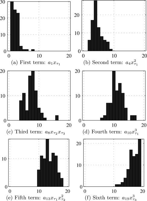
To select the six terms for the model, we proceed as follows. For j = 1, …, 6, we construct a histogram of those terms from Eq. 3 which occur as the $j\mathrm{th}$ term of a selected model. These are shown in Fig. 7. The most often retained monomials are collected to write the 6-term DDE

$$\begin{array}{cc}\multicolumn{1}{c}{\dot{x}}& \hfill =a_1{x}_{{\tau }_1}+a_2{x}_{{\tau }_1}^2+a_3{x}_{{\tau }_2}{x}_{{\tau }_3}\hfill \\ \multicolumn{1}{c}{\hspace{0.17em}}& \hfill +a_4{x}_{{\tau }_1}^3+a_5{x}_{{\tau }_1}{x}_{{\tau }_2}^2+a_6{x}_{{\tau }_3}^3\hfill \end{array}$$ (4)

actually used for discriminating control subjects from PD patients. It is interesting to note that when the selection process is run on only the $6\times 7=42$ time series recorded from controls, or alternatively on the 42 time series from PD patients, the same 6-term model is selected in both cases.

Figure 7.

(Color online) Histograms for the retained monomials in the 19-term DDE (3) for the 84 runs of the structure selection algorithm on group ii data sets. The x-axis is the index of monomials as in Eq. 3.

This indicates that the selected model structure captures finger-tapping dynamics regardless of the presence of the disease.

Selecting the delays from group ii

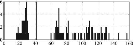
In contrast to the model structure, the delays selected by the GA depend on the data (controls, PDs, or both) used: The delays selected from the 42 data files of the PD patients are (22, 60, and 105), the delays selected from the 42 data files of the controls are (0, 29, and 41), and the delays selected from the whole data set of 84 files are (0, 23, and 41). Fig. 8 shows the histogram used to select the delays from the 42 data files of the controls.

Figure 8.

(Color online) Histograms of the delays for the 42 data files of the controls. The numbers on the x-axis are the delays and the numbers on the y-axis are the number of occurrences. The dominant three peaks are $\mathbf{\tau }=(0,29,41)$.

To discriminate control subjects from PD patients, we used the coefficient space of model (4), that is, the six-dimensional space ${\mathbb{R}}^6(a_1,a_2,...,a_6)$. For each session, the vector of coefficients $\{a_i\}$ was estimated using a SVD, defining one point—the center of the cloud of points generated from the sliding window positions—in the coefficient space.

In order to test the performance of the selected delays, a K-fold cross-validation^{44, 45} was used. The model coefficients $\mathbf{a}=(a_1,a_2,...,a_6)$ were split into K subsamples ${\mathbf{a}}_{K,n}$ (each subsample is one control subject and one PD subject). We have K = 6 for group i and K = 7 for group ii according to the number of patients for each condition in each group. Each of the K subsamples consists of n outputs ${\mathbf{a}}_n$, one a for each time series.

From the K subsamples, a single subsample ${\mathbf{a}}_n$ was retained as the validation data for testing the model and the remaining K – 1 subsamples were used as training data. For each validation, the K – 1 PD patients and the K – 1 control subjects were used to estimate an hyperplane splitting control subjects from PD patients. The hyperplane was obtained by running a linear support vector machine (SVM) (Refs. ^{46, 47, 48}).

For each partition, the model was fit to the training data, and then the model quality assessed on the validation data by computing the area under the receiver operating characteristic (ROC) curves, A′.⁴⁹ A ROC curve is a plot of the cumulative distribution function $P_1$ of the first class against the cumulative distribution function $P_2$ of the second class (see Ref. 49, p. 173 for exact definitions). In our case, we plotted the function $P_{\mathrm{CO}}$ of the control subjects against the function $P_{\mathrm{PD}}$ of the PD patients. To compute the area $A\text{'}$ under the ROC curve (following the approach introduced in Ref. 49), we ranked the outputs of SVM from the largest positive value to the most negative value. Let $r_i$ be the rank of the ith control subject point. The area under the ROC curve is approximated by

$$A\text{'}=\frac{S_0-n_0(n_0+1)/2}{n_0{n}_1},$$ (5)

where $S_0$ is the sum of the ranks of the control subject points, $n_0$ the number of control subject, and $n_1$ the number of PD patients. The cross-validation process was repeated $K^2$ times for all possible combinations of training and validation sets. The average of all $K^2$ cross-validations is then the model quality $\overline{A\text{'}}$. This method has the advantage that all observations are used for both training and validation.

From the average value $\overline{A\text{'}}$ reported in Table TABLE IV., it clearly appears that classification performance is better for group i than for group ii. Moreover, the delays estimated with control subjects provide better results than using those estimated with PD patients. This means that the delays estimated from the control group can serve as a dynamical “baseline” that captures dynamical information about the nonlinear dynamics of healthy subjects. Any departure from this baseline can then be used to assess the severity of the disease.

TABLE IV.

Delays and model quality. $\overline{A\text{'}}$ for the different sets of delays obtained from group ii data sets. $\overline{A\text{'}}$ is the mean value of the estimates $A\text{'}$ of the area under the ROC curves⁴⁹, ⁵⁰ according to Eq. 5 from a K-fold cross-validation framework.

Cohort	${\tau }_1$	${\tau }_2$	${\tau }_3$	$\overline{A\text{'}}$
				Group i	Group ii
PD patients	22	60	105	0.75	0.61
Control subjects	0	29	41	0.95	0.84
Patients and controls	0	23	41	0.94	0.74

We performed a second K-fold, leave-one-out cross-validation,⁵⁰ as follows. The subsamples are made of one PD patient or one control subject. Results are reported in Table TABLE V., where the control subjects from group ii were used for selecting the optimal delays. The sensitivity value 0.57 in Table TABLE V. means, surprisingly, that the model—its structure and delays—selected from group ii data sets was not able to accurately discriminate patients and control subjects of the same group. However, we have seen from Table TABLE III. that for group ii, the standard deviation of the UPDRS finger-tapping scores is 0.4 whereas the corresponding figure for group i is double that, at 0.8. A smaller standard deviation suggests that it should be harder to discriminate amongst group ii patients than amongst group i patients. This is consistent with the low sensitivity score in Table TABLE V..

TABLE V.

Statistics on the predictive accuracy obtained with model (4) and delays selected using the control subjects from group ii.

	Group i	Group ii
Sensitivity	0.95	0.57
Specificity	0.83	0.79

Comparison of UPDRS, HY, and DDE scores

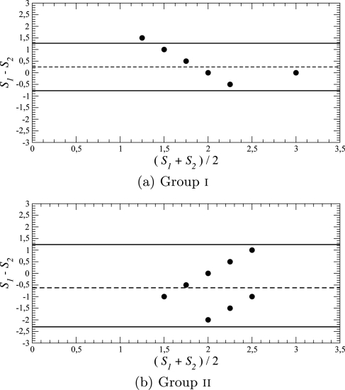
Although the UPDRS scale is known to be more reliable than the HY-scale,¹⁴ the latter is still widely used. In the case of group i, the two scales are significantly correlated (r = 0.80 and $p<0.0002$), whereas for group ii, the correlation is very poor (r = 0.330 and p = 0.2). In addition, a Bland-Altman test⁵¹ reveals that for both groups, there is a general correspondence between the two clinical measures with, in group i, a single point slightly outside the 95% confidence limit (Fig. 9a).

Figure 9.

Comparing the UPDRS finger-tapping ratings and HY ratings for Parkinson’s disease. Difference plotted versus mean, where $S_1=S_{\mathrm{UPDRS}}$ and $S_2=S_{\mathrm{HY}}$. The solid horizontal lines indicate the 95% confidence limits. The dashed lines indicate the mean difference: positive for group i and negative for group ii.

For every subject, there are up to 3 time-series from the dominant hand but due to windowing, each time-series generates a cloud of 6-dimensional points in coefficient space. Each cloud was replaced by its center-point, giving up to 3 points in coefficient space for every subject, both controls and PD. To define a central point for the 13 controls, we took the center of these center-points and used this as the central point, or base, for controls. The 1-dimensional DDE scores for the PD patients are then defined to be the distance Δ from the PD center-points for each time series to this base point for controls.

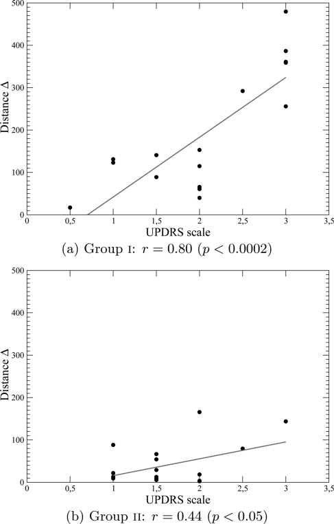
For group i, distances Δ are significantly correlated ($r=0.80\mathrm{and}p<0.0002$) with the UPDRS finger tapping scores (Fig. 10a). To be able to directly compare the distance Δ to the UPDRS scale using a Bland-Altman test, we inverted the linear regression

$$\Delta =-99+141S_{\mathrm{UPDRS}}$$ (6)

to obtain a rescale distance

$$\tilde{S}=\frac{\Delta +99}{141}.$$ (7)

We thus obtained an assessment of the Parkinson’s disease finger-tapping dysfunction which correlates better with the UPDRS finger tapping scale than HY-scale (Fig. 11). Such a comparison is not reasonable with results for group ii since (Fig. 10b) shows that the correlation between the UPDRS finger tapping scale and distance Δ is rather low (r = 0.44 and $p<0.05$). It is rather difficult to validate our scorings using a DDE because there is no obvious “gold standard” to use as a reference. The quite different results obtained with the two groups of patients may result from the difference in the UPDRS finger-tapping scores: compared to the HY-scale, these scores overestimate the severity of Parkinson’s disease for group i and underestimate it for group ii (Figs. 9a, 9b). Moreover the 95% confidence limits are $\pm 1$ for group i and $\pm 1.5$ for group ii. Our technique provides a measure which we have shown is related to Parkinson’s disease severity, but a larger group of patients will be needed to obtain a better estimation.

Figure 10.

(Color online) Comparing the UPDRS and DDE ratings for Parkinson’s disease finger-tapping.

Figure 11.

Comparing the UPDRS and DDE ratings for Parkinson’s disease finger-tapping: Difference versus mean. $S_1=S_{\mathrm{UPDRS}}$ and $S_2=\tilde{S}$. Data sets from group i.

Comparison of UPDRS and DDE scores for groups i and ii combined

Clinically, the mean scores for each subject are the main item of interest, so we plotted, for all subjects from groups i and ii together, the mean DDE distance $\overline{\Delta }$ vs. the mean UPDRS finger-tapping score. This plot is not shown but was similar to the plots in Fig. 10. The linear regression was obtained, as in Eq. 6, and then inverted, as in Eq. 7, to give the DDE-rescaled distance

$${\tilde{S}}_G=1+\overline{\Delta }/150.$$ (8)

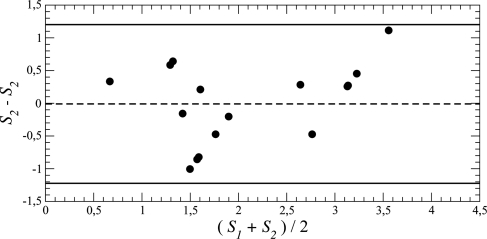
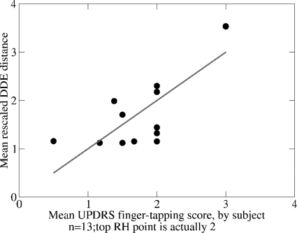
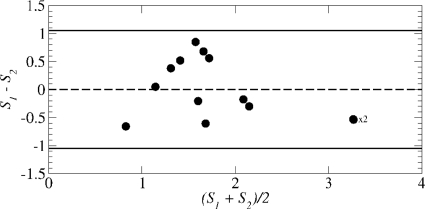
Fig. 12 shows ${\tilde{S}}_G$ plotted against the mean UPDRS finger-tapping score. The regression line is the diagonal, due to the rescaling, and the two scales are significantly correlated (r = 0.78 and $p<0.0015$). (Note that r is invariant under rescaling.) The difference vs. means plot (Fig. 13) has a 95% confidence limit = 1.05, slightly less than the confidence limit 1.2 for the group i ratings (Fig. 11). This 95% confidence limit is just over 25% of the range [0, 4], which, being less than 30%, is considered an acceptable percentage value when introducing a new measurement technique in cardiology.⁵⁵

Figure 12.

(Color online) Comparing the mean rescaled DDE and mean UPDRS, finger-tapping ratings for all subjects from groups i and ii combined: $r=0.785(p<0.0015)$.

Figure 13.

Comparing the mean rescaled DDE and mean UPDRS finger-tapping ratings for all subjects together: Difference versus mean. $S_1={\tilde{S}}_G$ and $S_2=\overline{S_{\mathrm{UPDRS}}}$. 95% confidence limit = 1.05.

CONCLUSION

Basic findings

An objective assessment of the severity of Parkinson’s disease is needed to augment clinical evaluations which are time consuming, expensive, and present inter-rater variability. We proposed a novel algorithmic means of assessing PD motor dysfunction through use of dynamical models based on delay differential equations. In this method, we selected the best structure of a nonlinear delay differential equation using a genetic algorithm fitted to a given movement time series. The coefficients of the nonlinear delay differential equation then were used as a six-dimensional numerical descriptor of the movement. This method was applied to repetitive finger-to-thumb tapping movements of PD patients and matched control subjects. We showed that under certain conditions—when there was substantial variation in disease severity across PD patients within a group and a small rate of marker occlusions—it was possible to obtain a structure for the model which, when associated with appropriate time delays, adequately discriminated PD patients from control subjects. When we compared the algorithmic scores derived with our method with clinical rating scales of PD motor severity, we found that the algorithmic scores compared favorably with the unified Parkinson’s disease rating scale. Finally, when we took a subject-centered view of our results and compared each subject’s mean rescaled DDE score with each subject’s mean UPDRS score, we obtained a correlation of 0.785 ($p<0.0015$), which shows that our DDE-based algorithmic scoring technique could be considered clinically acceptable.

The method for non-linear dynamical analysis of movement presented here can be used to characterize and assess not only the degree of dysfunction of movements of Parkinson’s patients but also the nature of the movement structure of a wide variety of motor disorders, including the movement dysfunction due to stroke, or that due to developmental motor dysfunction in childhood. Such quantitative and objective non-linear dynamical analysis can provide a new tool for clinicians to use in tracking recovery of function, progression of dysfunction, or the effectiveness of medical, surgical, or physical treatments in reversing dysfunction.

Study limitations

The total number of PD patients tested was small, six patients in group i, and seven in group ii. A much larger sample size will be needed to more fully determine the reliability of our classification technique. Moreover, the data collection protocols we used differed slightly for the two groups of patients studied: group i data were recorded at 120 Hz and group ii at 480 Hz. This difference in sampling rate might have led to the greater number of marker occlusions observed in the recordings of group i, an effect accentuated after upsampling to 480 Hz. Alternatively, the greater number of marker occlusions in group i may have resulted from group i patients having greater PD severity than those of group ii. More severely affected patients often rotate their hands or otherwise occlude view of one of the markers at certain points during the movement. Having groups differing in motor severity, even within the same overall stage of the disease, allowed us to examine our method across a wider range of motor deficits in PD patients who are clinically typical, and without the cognitive and emotional decline that occurs in more advanced stages of the disease. We also note that most aspects of the data collection protocols for the two groups were virtually identical: The same 12 camera opto-electronic 3D movement tracking system was used for both groups; IREDs were affixed in the same locations on the index finger and thumb and in the same manner, for both groups; data were collected in the same experimental room in both groups; the same duration of the finger tapping movement was recorded for each group; the same patient selection criteria were used for each group, namely, diagnosis of typical, idiopathic Parkinson’s disease of Hoehn and Yahr stage II-III in severity (mild to moderate); patients in both groups were tested at least 12 h off of their anti-parkinsonian medications; testing sessions occurred in the mornings; and control subjects were age-matched to the PD patients in the same manner for both groups.

A further limitation of our study is that the clinical rating scales used, the UPDRS and the Hoehn and Yahr scales, provide only somewhat global measures of motor severity. The UPDRS is the most widely used scale for rating PD severity, but even its functional divisions of deficits are quite broad (e.g., mild, moderate, or severe). The UPDRS has recently undergone a movement disorders society-sponsored revision to correct identified shortcomings.⁵² This revised scale has been undergoing clinimetric testing and is beginning to be used clinically. Use of such enhanced clinical rating scales could provide a more precise and objective reference for comparison with our algorithmically derived scores, and thus, to more adequately assess the reliability of our classification technique.

Future studies

Future investigations planned in our laboratory will test not only finger tapping movements but also a variety of other repetitive movements that are also impaired in PD, such as rapid, alternating forearm supination-pronation. Currently, it still is an open question whether individual finger tapping is sufficient to evaluate the severity of Parkinson’s disease. The non-linear dynamical analysis presented here could also be used to help determine the effects of aging on loss of sensorimotor function. It is known that sensorimotor function degrades with aging.⁵³ Moreover, in normal aging, we lose approximately 4.7% of our dopamine-containing cells per decade,⁵⁴ and, indeed, a key element of Parkinson’s disease is the age-dependent reduction of dopamine coupled to a disease process that produces an exponential loss of dopamine cells.⁵⁴ Thus, elderly subjects provide a naturally occurring condition of mild dopamine depletion that is associated with loss of sensorimotor function. However, the degree of motor dysfunction at various age spans has not been systematically characterized. Use of the non-linear, dynamical analysis presented here could help provide such a systematic characterization. Likewise, the techniques presented here could be used to characterize and assess the degree of motor dysfunction in a wide range of motor disorders, varying from motor disorders due to stroke to those due to developmental childhood disorders.

DDE data analysis technique used in this paper

The technique described here, using GAs to find a DDE model that can be used as classifier, has been used previously^{24, 25, 26} and is currently being improved and applied to various medical data sets. Technical and mathematical details of this technique and further applications are under investigation and are planned to be published separately.

References

- Rodriguez-Oroz M. C., Jahanshahi M., Krack P., Litvan I., Macias R., Bezard E., and Obeso J. A., Lancet Neurol. 8(12 ), 1128 (2009). 10.1016/S1474-4422(09)70293-5 [DOI] [PubMed] [Google Scholar]
- Rivlin-Etzion M., Marmo O., Heimer G., Raz A., Nini A., and Bergman H., Curr. Opin. Neurobiol. 16, 629 (2006). 10.1016/j.conb.2006.10.002 [DOI] [PubMed] [Google Scholar]
- Brown R. G. and Marsden C. D., Trends Neurosci. 13(1 ), 21 (1990). 10.1016/0166-2236(90)90058-I [DOI] [PubMed] [Google Scholar]
- Benecke R., Rothwell J. C., Dick J. P. R., Day B. L., and Marsden C. D., Brain 110(2 ), 361 (1987). 10.1093/brain/110.2.361 [DOI] [PubMed] [Google Scholar]
- Flowers K. A., Brain 99(2 ), 269 (1976). 10.1093/brain/99.2.269 [DOI] [PubMed] [Google Scholar]
- Adamovich S. V., Berkinblit M. B., Hening W., Sage J., and Poizner H., Neuroscience 104(4 ), 1027 (2001). 10.1016/S0306-4522(01)00099-9 [DOI] [PubMed] [Google Scholar]
- Poizner H., Feldman A. G., Levin M. F., Berkinblit M. B., Hening W. A., Patel A., and Adamovich S. V., Exp. Brain Res. 133(3 ), 279 (2000). 10.1007/s002210000379 [DOI] [PubMed] [Google Scholar]
- Schettino L., Adamovich S., Hening W., Tunik E., Sage J., and Poizner H., Exp. Brain Res. 168, 186 (2006). 10.1007/s00221-005-0080-4 [DOI] [PubMed] [Google Scholar]
- Tunik E., Feldman A. G., and Poizner H., Parkinsonism and Related Disorders 13(7 ), 425 (2007). 10.1016/j.parkreldis.2007.02.003 [DOI] [PMC free article] [PubMed] [Google Scholar]
- Hoehn M. and Yahr M., Neurology 17(5 ), 427 (1967). [DOI] [PubMed] [Google Scholar]
- Jankovic J., McDermott M., Carter J., Gauthier S., Goetz C., Golbe L., Huber S., Koller W., Olanow C., Shoulson I., Stern M., Tanner C., and Weiner W., Neurobiology 40(10 ), 1529 (1990). [DOI] [PubMed] [Google Scholar]
- Goetz C. G., Poewe W., Rascol O., Sampaio C., Stebbins G. T., Counsell C., Giladi N., Holloway R. G., Moore C. G., Wenning G. K., Yahr M. D., and Seidl L., Mov Disord. 19(9 ), 1020 (2004). 10.1002/mds.v19:9 [DOI] [PubMed] [Google Scholar]
- Fahn S., Elton R. L., and UPDRS program members, “Unified Parkinson’s disease rating scale,” in Recent Developments in Parkinson’s Disease, edited by Fahn S., Marsden C. D., Goldstein M., and Calne D. B. (Macmillan Healthcare Information, Florham Park, NJ, 1987), Vol. 2, pp. 153–163 and 293–304. [Google Scholar]
- Ramaker C., Marinus J., Stiggelbout A. M., and van Hilten B. J., Mov Disord. 17(5 ), 867 (2002). 10.1002/(ISSN)1531-8257 [DOI] [PubMed] [Google Scholar]
- Ginanneschi A., Degl’Innocenti F., Magnolfi S., Maurello M. T., Catarzi L., Marini P., and Amaducci L., Neuroepidemiology 7, 38 (1988). 10.1159/000110159 [DOI] [PubMed] [Google Scholar]
- Richards M., Marder K., Cote L., and Mayeux R., Mov Disord. 9(1 ), 89 (2004). 10.1002/(ISSN)1531-8257 [DOI] [PubMed] [Google Scholar]
- Giuffrida J. P., Riley D. E., Maddux B. N., and Heldman D. A., Mov Disord. 24(5 ), 723 (2009). 10.1002/mds.v24:5 [DOI] [PubMed] [Google Scholar]
- Salarian A., Russmann H., Wider C., Burkhard P. R., Vingerhoets F. J., and Aminian K., IEEE Trans. Biomed. Eng. 54(2 ), 313 (2007). 10.1109/TBME.2006.886670 [DOI] [PubMed] [Google Scholar]
- Rivière C. N., Reich S. G., and Thakor N. V., J. Neurosci. Methods 74(1 ), 77 (1997). [DOI] [PubMed] [Google Scholar]
- Langston J., Widner H., Goetz C., Brooks D., Fahn S., Freeman T., and Watts R., Mov Disord. 7(1 ), 2 (1992). 10.1002/(ISSN)1531-8257 [DOI] [PubMed] [Google Scholar]
- Maquet J., Letellier C., and Aguirre L. A., J. Math. Biol. 55(1 ), 21 (2007). 10.1007/s00285-007-0075-9 [DOI] [PubMed] [Google Scholar]
- Aguirre L. A., Letellier C., and Maquet J., Sol. Phys. 241, 103 (2008). 10.1007/s11207-008-9160-5 [DOI] [Google Scholar]
- Letellier C., Aguirre L. A., and Freitas U. S., Chaos 19, 023103 (2009). 10.1063/1.3125705 [DOI] [PubMed] [Google Scholar]
- Kadtke J., Phys. Lett. A 203(4 ), 196 (1995). 10.1016/0375-9601(95)00375-D [DOI] [Google Scholar]
- Lainscsek C., Letellier C., Kadtke J., Gouesbet G., and Schürer F., Phys. Lett. A 265, 264 (2000). 10.1016/S0375-9601(99)00893-2 [DOI] [Google Scholar]
- Lainscsek C. and Gorodnitsky I., “Characterization of various fluids in cylinders from dolphin sonar data in the interval domain,” in Oceans 2003: Celebrating the Past. Teaming Toward the Future (Marine Technology Society/IEEE, 2003), Vol. 2, pp. 629–632. [Google Scholar]
- Agostino R., Berardelli A., Currà A., Accornero N., and Manfredi M., Mov Disord. 13(3 ), 418 (1998). 10.1002/mds.870130308 [DOI] [PubMed] [Google Scholar]
- Agostino R., Curra A., Giovannelli M., Modugno N., Manfredi M., and Berardelli A., Mov Disord. 18(5 ), 560 (2003). 10.1002/(ISSN)1531-8257 [DOI] [PubMed] [Google Scholar]
- Lukos J. R., Lee D., Poizner H., and Santello M., PLoS ONE 5(2 ), e9184 (2010). 10.1371/journal.pone.0009184 [DOI] [PMC free article] [PubMed] [Google Scholar]
- Takens F., Lect. Notes Math. 898, 366 (1981). 10.1007/BFb0091903 [DOI] [Google Scholar]
- Kremliovsky M., Kadtke J., Inchiosa M., and Moore P., Int. J. Bifurcation Chaos Appl. Sci. Eng. 8(4 ), 813 (1998). 10.1142/S0218127498000619 [DOI] [Google Scholar]
- Kadtke J. and Kremliovsky M., Phys. Lett. A 260(3–4 ), 203 (1999). 10.1016/S0375-9601(99)00527-7 [DOI] [Google Scholar]
- Cao L., Physica D 110(1 and 2 ), 43 (1997). 10.1016/S0167-2789(97)00118-8 [DOI] [Google Scholar]
- Letellier C., Maquet J., Le Sceller L., Gouesbet G., and Aguirre L. A., J. Phys. A 31, 7913 (1998). 10.1088/0305-4470/31/39/008 [DOI] [Google Scholar]
- Letellier C., Aguirre L. A., and Maquet J., Phys. Rev. E 71, 066213 (2005). 10.1103/PhysRevE.71.066213 [DOI] [PubMed] [Google Scholar]
- Letellier C. and Aguirre L. A., Chaos 12, 549 (2002). 10.1063/1.1487570 [DOI] [PubMed] [Google Scholar]
- Lainscsek C., Letellier C., and Gorodnitsky I., Phys. Lett. A 314(5–6 ), 409 (2003). 10.1016/S0375-9601(03)00912-5 [DOI] [Google Scholar]
- Judd K. and Mees A. I., Physica D 120, 273 (1998). 10.1016/S0167-2789(98)00089-X [DOI] [Google Scholar]
- Judd K. and Mees A. I., Physica D 82, 426 (1995). 10.1016/0167-2789(95)00050-E [DOI] [Google Scholar]
- Aguirre L. A. and Billings S. A., Int. J. Control 62(3 ), 569 (1995). 10.1080/00207179508921557 [DOI] [Google Scholar]
- Goldberg D., Genetic Algorithms in Search, Optimization and Machine Learning (Addison-Wesley, Boston, MA, 1989). [Google Scholar]
- Holland J. H., Adaptation in Natural and Artificial Systems (MIT, Cambridge, MA, 1992). [Google Scholar]
- Press W., Flannery B., Teukolsky S., and Vetterling W., Numerical Recipes in C (Cambridge University Press, 1992). [Google Scholar]
- Stone M., J. R. Stat. Soc. Ser. B (Methodol.) 36(2 ), 111 (1974). [Google Scholar]
- Kohavi R., in Proceedings of the 14th International Conference on Artificial Intelligence (IJCAI) (Morgan Kaufmann, Los Altos, CA, 1995), pp. 1137–1143.
- Vapnik V. and Lerner A., Autom. Remote Control 24, 774 (1963). [Google Scholar]
- Vapnik V. and Chervonenkis A., Theory of Pattern Recognition (Nauka, Moscow, Russia, 1974). [Google Scholar]
- Cortes C. and Vapnik V., Mach. Learn. 20(3 ), 273 (1995). [Google Scholar]
- Hand D. J. and Till R. J., Mach. Learn. 45, 171 (2001). 10.1023/A:1010920819831 [DOI] [Google Scholar]
- Wu C. F. J., Ann. Stat. 14(4 ), 1261 (1986). 10.1214/aos/1176350142 [DOI] [Google Scholar]
- Bland J. M. and Altman D. G., Lancet 1(8476 ), 307 (1986). 10.1016/S0140-6736(86)90837-8 [DOI] [PubMed] [Google Scholar]
- Goetz C. G., Fahn S., Martinez-Martin P., Poewe W., Sampaio C., Stebbins G. T., Stern M. B., Tilley B. C., Dodel R., Dubois B., Holloway R., Jankovic J., Kulisevsky J., Lang A. E., Lees A., Leurgans S., LeWitt P. A., Nyenhuis D., Olanow C. W., Rascol O., Schrag A., Teresi J. A., Van Hilten J. J., and LaPelle N., Mov Disord. 22(1 ), 41 (2007). 10.1002/(ISSN)1531-8257 [DOI] [PubMed] [Google Scholar]
- Sasaki H., Masumoto J., and Inui N., Motor Control 15(2 ), 175 (2011). [DOI] [PubMed] [Google Scholar]
- Fearnley J. M. and Lees A. J., Brain 114(Pt 5 ), 2283 (1991). 10.1093/brain/114.5.2283 [DOI] [PubMed] [Google Scholar]
- Critchley L. A. H. and Critchley J. A. J. H., J. Clin. Monit Comput. 15(2 ), 85 (1999). 10.1023/A:1009982611386 [DOI] [PubMed] [Google Scholar]
- S. Luke, Essentials of Metaheuristics (Lulu.com, 2011), http://cs.gmu.edu/∼ sean/book/metaheuristics/
- Vose M. D., The Simple Genetic Algorithm: Foundations and Theory (MIT, Cambridge, MA, 1999). [Google Scholar]
- Rahmat-Samii Y. and Michielssen E., Electromagnetic Optimization by Genetic Algorithms (Wiley, New York, 1999). [Google Scholar]