Dynamic noise, chaos and parameter estimation in population biology

Abstract

We revisit the parameter estimation framework for population biological dynamical systems, and apply it to calibrate various models in epidemiology with empirical time series, namely influenza and dengue fever. When it comes to more complex models such as multi-strain dynamics to describe the virus–host interaction in dengue fever, even the most recently developed parameter estimation techniques, such as maximum likelihood iterated filtering, reach their computational limits. However, the first results of parameter estimation with data on dengue fever from Thailand indicate a subtle interplay between stochasticity and the deterministic skeleton. The deterministic system on its own already displays complex dynamics up to deterministic chaos and coexistence of multiple attractors.

1. Introduction

A major contribution to stochasticity in empirical epidemiological data is population noise, which is modelled by time-continuous Markov processes or master equations [1–3]. In some cases, the master equation can be analytically solved and from the solution a likelihood function be given [4]. The likelihood function gives best estimates via maximization or can be used in the Bayesian framework to calculate the posterior distribution of parameters [3]. Here, we start with an example of a linear infection model that can be solved analytically in all aspects and then generalize to more complex epidemiological models that are relevant for the description of influenza or dengue fever [5], on the cost of having to perform more and more steps by simulation to obtain the likelihood function by complete enumeration [6] or even in extreme cases just to search for the maximum.

Recent applications to a multi-strain model applied to empirical datasets of dengue fever in Thailand, where the model displays such complex dynamics as deterministic chaos in wide parameter regions [5,7], including coexistence of multiple attractors, e.g. in isolas [8], stretch the presently available methods of parameter estimation well to its limits. Finally, the analysis of scaling of solely population noise indicates that very large world regions have to be considered in data analysis in order to be able to compare the fluctuations of the stochastic system with the much easier to analyse deterministic skeleton. Such a deterministic skeleton can already show deterministic chaos [9,10], here via torus bifurcations [8], which are also found in other ecological models, such as the seasonally forced Rosenzweig–McArthur model [11].

The main aim of this contribution is to give an overview and didactic introduction to parameter estimation in population biology from simple analytically solvable cases to recently developed numerical methods applicable to larger models with such complex dynamical behaviour as deterministic chaos in its mean field deterministic skeleton. Although this is a review some new results will be presented here as well, mainly to include dynamic noise in the likelihoods of the numerical simulations of complex models in parallel with the first given analytical results in the simple models.

2. An analytically solvable case

We first review some of the simplest epidemiological models, and show explicitly the relation between the formulation as a stochastic process and the deterministic models formulated as ordinary differential equation (ODE) systems. Then we will solve explicitly one example where all steps towards a closed solution can be given analytically. In this example model, a likelihood function can be derived, including an analytical expression of, as well as the maximum likelihood best estimate as, a full Bayesian formulation.

The model can be generalized to give a fast approximation scheme for more complicated stochastic epidemic models which later will be used in the applications with likelihoods based on simulations. With such simulation models, all steps, which we show in the analytically solvable case, can be performed in more complicated models and applied to time series of real disease cases.

2.1. Basic epidemiological models including population noise

The simplest closed epidemiological model is the susceptible–infected–susceptible (SIS) model for susceptible and infected hosts, specified by the following reaction scheme:

2.1

for stochastic variables I and with N the total population size of hosts. The transitions are infection rate β and recovery rate α. From the reaction scheme, we can give the dynamics of the probabability p(I, t) as follows:

2.2

With the definition of mean values, which is given here by 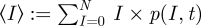, we can derive the dynamics of the mean number of infected in time by inserting the dynamics of the probability given above and obtaining after some calculation (for a more extended derivation and further details, see Stollenwerk & Jansen [3] and references therein)

2.3

where higher moment now appears in the dynamics. For dynamics of higher moments and in spatial systems, see the studies by Stollenwerk & Jansen [3] and Stollenwerk et al. [12] for the equivalent higher clusters (pairs, triples, etc.). Since, in spatial systems, the epidemiological thresholds are, in general, shifted away from the mean field values, further methods valid at and around these thresholds can be used [13].

To obtain a closed ODE, we neglect the variance, restricting the dynamics to its simplest deterministic part, the so-called mean field approximation, and find the famous logistic equation (in a slightly unusual form but mathematically equivalent to the well-known formulation of Verhulst)

2.4

In complete analogy, many other epidemiological models can be formulated, often with somewhat more effort, such as the susceptible–infected–recovered (SIR) epidemic for susceptible, infected and recovered hosts

2.5

with the respective transition rates, infection rate β, recovery rate γ and waning immunity α. For variables S and I with given from the previous two classes, we can again give the dynamics of the probabability p(S, I, t) by

2.6

And, again, the mean field approximation of now higher cross moments such as 〈SI〉 gives a well-known closed ODE system for this SIR system.

A seasonally forced SIR system can already be used to analyse diseases such as influenza with available long time series from various countries [14]. As we will show later, in realistic parameter regions for influenza, we find complex dynamic behaviours with bifurcations from limit cycles to double limit cycles and up to deterministically chaotic dynamics. Also, multi-strain epidemic models can be formulated in the frame work of stochastic processes given above by including host classes of infected with one or another strain.

One example is a dengue model, which can capture differences between primary and secondary infection, an important feature owing to the so-called antibody-dependent enhancement (ADE). Infected with one strain are labelled and infected with a second different strain ; they can recover from that strain, called and , respectively, and after a period of temporary cross immunity become susceptible to infection with another strain. 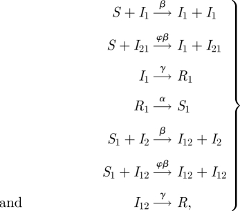Hence, a susceptible that has been infected with strain 1 previously is labelled , and can now only be infected with strain 2, therefore becomes , etc. For details, see Aguiar et al. [5] and references therein. The reaction scheme then looks for an infection with one strain and a subsequent infection with a second strain, such as

2.7

leading to a 10-dimensional ODE system which can be reduced to 9 d.f. for constant population size. Already in its simplest form, the model shows complex dynamics in wide parameter regions, up to deterministic chaos characterized by positive Lyapunov exponents [5]. A version of this model including seasonality and import can easily explain the fluctuations observed in time series of severe disease (dengue haemorrhagic fever; DHF) in Thailand [7]. We will come back later to these models. First, we will analyse a simpler model.

2.2. Analytical solution of the linear infection model

To simplify further for analytical tractability, we assume only infection and only from an outside population. This simplified epidemiological model, an SI system, where infection is acquired only from the outside, leads to a master equation which is linear not only in probability but also in the state variables. A linear mean field approximation for the dynamics of the expectation values [3] is obtained from this process. Although very simple in its set-up, it can be applied to real world data of influenza in certain stages of the underlying SIR model, when considering the cumulative number of infected cases during the outbreak [4]. The reaction scheme is given by

2.8

for infected I and susceptibles with population size N, and infection rate β as the only possible transition. The underlying model hypothesis is that infection can be acquired from outside the considered population of size N, hence meeting infected I*.

The master equation reads for the probability p(I, t)

2.9

which can be solved using the characteristic function

2.10

or approximated by Kramers–Moyal expansion to preserve eventual attractor switching in more complicated models, relevant for influenza [15].

2.3. Solving the master equation

For suitable initial conditions, the master equation can be solved to obtain the transition probabilities needed to construct the likelihood function. From the definition of the characteristic function, equation (2.10), we see immediately that its derivatives are related to the moments

2.11

and g itself is a discrete Fourier transform using the definition , hence

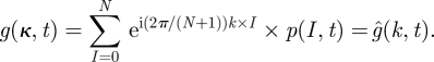2.12

Owing to this, we can, via Fourier back transform, obtain the probabilities once we know the characteristic function

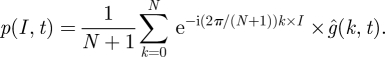2.13

Hence, we can derive a dynamics for the characteristic function from the dynamics of the probabilities, eventually solve the partial differential equation (PDE) for the characteristic function and then obtain, via Fourier back transform, the solution to the probability.

The dynamics of the characteristic function, obtained from the master equation, is

2.14

giving the PDE

using , and the initial condition , and hence as the initial condition for the characteristic function. With a classical separation ansatz and the given initial conditions, we can solve the PDE analytically, obtaining as the solution (figure 1a)

Figure 1.

(a) An example of the characteristic function in real and imaginary parts with fixed Δt given by the sampling rate of the time series. (b) From the characteristic function we can obtain the solution to the stochastic model and with it the likelihood function, as shown here with its best estimate of the model parameter as maximum.

Then an inverse Fourier transformation gives the transition probability , explicitly

as the solution to the master equation. Owing to the special initial conditions of exactly having I₀ infected at time t₀, this solution is at the same time the transition probability , as needed to construct the likelihood function for the parameter estimation.

2.4. Likelihood function from the master equation

From the transition probabilities, we can construct the likelihood function, i.e. the joint probability of finding all data points from our empirical time series interpreted as a function of the model parameters

2.15

With the analytical solution, we obtain here explicitly using

and can plot the likelihood as a function of the parameter, here β as shown in figure 1b, and its maximum as the best estimator . Here, the best estimator can be calculated analytically as well [3] by evaluating the first derivative of the likelihood to be zero at . We obtain analytically

2.16

as the best estimate for the parameter β.

2.5. Fisher information

To obtain an approximation of the confidence intervals in the frequentists' approach, after maximizing the likelihood, one assumes that the likelihood essentially reflects a Gaussian distribution, an assumption justified by the central limit theorem of probability in the case of many data points available for the likelihood. Hence

2.17

is a Gaussian distribution around the best estimate with a standard deviation σ to be obtained from the curvature of the likelihood around its maximum

We can test this assumption of Gaussianity and its performance by the following experiment: we simulate the stochastic process, i.e. the master equation via the Gillespie algorithms [16,17], many times and each time calculate the best estimate, obtaining a histogram of the estimates around the initial model parameter. Then we take one typical realization from the bulk of the distribution and calculate the Gaussian distribution around the best estimate with variance given by the negative inverse of the curvature of the likelihood, the Fisher information, and compare the Gaussian with the histogram of many realizations (figure 2). The comparison is relatively good, but the histogram and previously the likelihood function are slightly asymmetric around the maximum, requiring a refined approach to better capture the distribution of parameters given the experimental or empirical data. This can be achieved by using the Bayesian framework, as will be shown below.

Figure 2.

Comparison of the histogram of many realizations of best estimates (step-like curve) and a Gaussian distribution obtained from the best estimate and the Fisher information via the likelihood of one typical realization (smooth curve). The comparison is relatively good, but the histogram and previously the likelihood function are slightly asymmetric around the maximum.

2.6. Bayesian framework

The Bayesian framework starts by using the likelihood function interpreted as the probability of finding the data given a parameter (or parameter set in more general cases); hence with being the data vector and parameter β and constructs from it being the probability of the parameters conditioned on the present data, here from the time series of the epidemic system, the Bayesian posterior . This can be achieved only by imposing a prior , a probability of plausible parameter sets, hence we have the Bayes formula

2.18

with the likelihood function as before, and a normalization once a prior is specified. For analytical calculations, a so-called conjugate prior is often used, i.e. a distribution for the parameter in the same functional form as the parameter appears in the likelihood function, here a beta distribution. Then the posterior also has functionally the same form, here again a beta distribution, but the parameters, called hyperparameters, now contain information from the data points. For the linear infection model, all steps can still be performed analytically.

The posterior is given explicitly by

with hyperparameters and from the prior parameters a and b. For the detailed calculation, see Stollenwerk & Jansen [3]. One can observe that, for large datasets, the sums over the data points are giving much larger values in the hyperparameters than the original prior parameters, hence a soft prior is achieved. If the prior parameters are of the same order of magnitude as the terms originating from the data points, the prior determines much more the form of the posterior than the observations. Such hard priors are not always avoidable when only small datasets are available. Then, the posterior gives some indication of the underlying insecurities of the stochastic process but should also not be overinterpreted.

Figure 3 shows the comparison of a histogram of best estimates from many realizations of the stochastic process (red), information that is not usually given in most empirical systems; often, we only have a single realization, and the results from the parameter estimation, a Gaussian approximation from the best estimate and the Fisher information (green), and finally the Bayesian posterior (black) obtained from a conjugate prior (blue), which is here nicely broad, not imposing much restriction on the parameter values considered.

Figure 3.

Comparison between the maximum likelihood method and the Bayesian approach for a simple linear infection model, with all analytical tools available.

2.7. Some further remarks on empirical situations

Before continuing with more complex population models, we make some remarks on what can happen in empirical situations, which we illustrate here using analytical examples.

A parameter can be close to one of its boundaries and not well measured by the given data points. In figure 4, we show an example from a time series of independent exponentially distributed waiting times (a typical null model for spiking neurons). This model can also be treated analytically in the same way as the linear infection model, which we have calculated above explicitly. The only parameter a of this model is always positive. However, the approximation of the likelihood by a Gaussian distribution can have a large tail in the negative region of the parameter space (green curve). In this case, clearly, the histogram of our Gedanken experiment (red curve) is highly asymmetric, with a long tail shifted to the right, i.e. towards positive best estimates. Also the conjugate prior (blue curve) vanishes at , indicating that a negative value of a is meaningless in this model. The Bayesian posterior (black curve) captures the asymmetric distribution of estimates much better than the Gaussian approximation, on which the Fisher information is based, would suggest. Here, clearly the Bayesian approach is performing better, while the Gaussian approximation has a large tail for negative parameter a values.

Figure 4.

In an application to the situation of exponentially distributed waiting times, the effect of parameter boundaries on the parameter estimation can be studied.

Again, we illustrate the second remark on the previously studied linear infection model. Previously, we compared the histogram of many stochastic realizations with the likelihood of a ‘typical’ realization, by which we mean a realization close to the bulk of the histogram. However, in any empirical situation our only available dataset, let us say of an epidemiological or ecological time series, is more ‘atypical’ in the sense that it is still quite likely to be obtained under the model assumptions, but not coming from the central bulk. Just by using another seed of our random generator than the one used in figure 3, we obtain the situation shown in figure 5a. And we have to remember that, in empirical situations, we do not even have the histogram of our Gedanken experiment, hence we have the information from figure 5b only. A reasonable confidence interval still covers the true parameter value, i.e. the one we originally used to generate the model realization, but the maximum likelihood best estimate as well as the maximum of the Bayesian prior can be quite far away from that empirically unknown true parameter value.

Figure 5.

An ‘atypical’ realization is often encountered in empirical studies, where we have only one dataset available. (a) Frequentists' and Bayesian approach to a dataset from the right tail of the histogram, which still has a high probability to be obtained. (b) Empirically, we usually do not have the information of the Gedanken experiment, the histogram of the best estimates from many realizations of our underlying process.

As a third remark, we already mention here that the binomial transition probability from the linear infection model can be generalized to a numerical approximation scheme for more complex models, the so-called Euler multi-nomial approximation. The assumption of linear transition rates holds for short time intervals and gives a binomial transition rate for staying in the present state or moving into one other or a multi-nomial for leaving to more than one other state. We will use this Euler multi-nomial approximation later for numerical parameter estimation in an SIR model.

3. Numerical likelihood via stochastic simulations

In cases where not all steps or even no step can be performed analytically, a comparison of stochastic simulations, depending on the model parameters, with the empirical data is the only available information on the parameters. One can compare many simulations and see if they fall within a region around the data, called η-ball, depending on the parameter set used for the simulations [6] obtaining estimates of the likelihood function. In figure 6, an SIR model is compared with empirical data from influenza; here, owing to the relative simplicity of the stochastic model, a numerical enumeration of the whole relevant parameter space is still computationally possible (equivalent to a flat but cut-off prior). In more complicated models, dengue fever models and data from Thailand, a complete enumeration of the parameter space is not computationally possible, although only six parameters and nine initial conditions have to be estimated. Particle filtering, i.e. an often quite restricted distribution of parameters and initial conditions, a hard prior in Bayesian language, is stochastically integrated and compared with the empirical time series, selecting the best performers as the maximum of the likelihood function.

Figure 6.

Application of the numerical likelihood estimation of the infection rate and the initial number of susceptibles on influenza data from InfluenzaNet, an Internet-based surveillance system (EPIWORK project).

In figure 6, we can also study confidence intervals for multiple parameters. The easiest generalization from the one-parameter case is the likelihood slice, in which around the maximum all but one parameter are fixed and then the confidence interval is evaluated for the remaining parameter, as in the one-parameter case. In figure 6, the maximum of the likelihood is not easily determined and we observe near equally likely parameter sets along a long comb.

To quantify this insecurity along the comb better, one can fix one parameter for which the confidence interval is to be determined, and maximize all the other parameters, which gives essentially a projection of the comb in figure 6. A so-called likelihood profile is obtained in this way. This method gives large confidence intervals for the two parameters chosen here, the infection rate and the initial number of susceptibles before the influenza season, quantifying well the insecurity of parameters rather than what the eventually much smaller likelihood sections would suggest.

3.1. Application to more complex models

In such cases, in which the model can display deterministic chaos, like the one in dengue fever that we investigated [5,7], even the short-term predictability and long-term unpredictability (as measured by the largest Lyapunov exponent) prohibit the comparison of stochastic simulations with the entire time series. Hence, iteratively short parts of the time series are compared with the stochastic particles, and, via simulated annealing, the variability of the particles is cooled down, i.e. the priors are narrowed in Bayesian language. The final method is called ‘maximum likelihood iterated filtering’ (MIF) [18–21]. We apply this method to dengue data from Thailand (a detailed manuscript is in preparation [22]), obtaining wide likelihood profiles for some of the parameters. Here, we display bifurcation diagrams obtained from the best estimates, around a difficult to estimate but important model parameter, the import rate ϱ (figure 7a) for the parameter set from data from a single province and (figure 7b) from a whole region with several provinces. We observe that the estimates are driven towards imports near the boundary towards extinction. Extrapolating finally to larger population sizes than the current data allow (figure 8) shows that, in such larger systems, a better estimate should be obtained in the region of complex dynamics since the boundary towards extinction is shifted towards smaller import values. For details of the stochastic bifurcation diagrams, see Aguiar et al. [23].

Figure 7.

Comparison of deterministic skeleton and stochastic simulations for bifurcation diagrams with estimated parameters for (a) dengue fever cases in the Chiang Mai province of Thailand and (b) dengue in the surrounding nine northern provinces of Thailand. The crucial parameter is the import ϱ. Even in systems with population sizes well above 1 million, the noise level of the stochastic system is enormous.

Figure 8.

Extrapolation of population sizes to (a) the whole of Thailand and (b) Thailand and its surrounding countries with ca 200 mio. inhabitants. The noise level of the stochastic simulation approaches the deterministic system only for very large system sizes.

To illustrate the ideas behind iterated particle filtering and including the explicit effects of dynamic noise as investigated in the previous example analytically, we will now look at a susceptible–infected–recovered–re-susceptible (SIRS) model with seasonality and import, which is motivated by recent studies on influenza [14] and which is reported to show deterministic chaos, and see how a suitable particle filter can perform in such a scenario.

4. A test case for iterated filtering under chaotic dynamics

Looking back to the roots of filtering in time-series analysis, the earliest complete filters are the Stratonovich–Kalman–Bucy filters [24–29], also known as Kalman filters, for linear stochastic systems under additional observation noise.

4.1. A brief look at the history of filtering

A state-space model with state vector x and noise vector ɛ and in the simplest case a linear scalar as observation with noise ξ can be solved explicitly to find , i.e. from the measurement y the underlying states x can be obtained, a task which often occurs in signal analysis in physics. But already including the estimation of parameters, here the matrix A, leads to a nonlinear problem that cannot be solved analytically, but has to be approximated, via extended Kalman filters; hence, the calculation of or is already non-trivial.

Similarly for nonlinear systems , where the parameter vector θ now replaces the coefficients of the matrices A and B, and observation has often been treated with simulation procedures to solve the classical filtering problem, i.e. to estimate the states x from the observations y, but turns out to be much more difficult, in computational terms, again for parameter estimation, i.e. to estimate θ from y, although it is tempting to just consider parameters as additional states and leave the conceptual framework unchanged. But then, as in MIF, the likelihood function only considers the observation noise, not the dynamic noise. In mathematical terms, the likelihood function is taken from the observation process and includes only indirectly the dynamic noise giving zero weight to dynamic realizations below the observations. For extended reviews on filtering, see [30–33].

We include dynamic noise explicitly in the iterated filtering with resampling and obtain good results for difficult-to-estimate parameters such as the import rate under chaotic dynamics.

4.2. Seasonal SIR model with chaotic dynamics

The SIR model with import ϱ

4.1

and seasonal forcing given by

4.2

and parameters in the uniform phase and chaotic amplitude (UPCA) region, relevant for influenza [14], , , , , shows around the import deterministic chaos. We take stochastic simulations from this model to test time series for the illustration of iterated filtering with dynamic noise in the likelihood function estimated via the Euler multi-nomial approximation, again a stochastic simulation method comparing the data by using an η-distance measure; see figure 9 for the comparison of the example dataset and the approximating simulation. They diverge because of the deterministically chaotic dynamics after about 2 years of the simulation, rather than because of the different simulation schemes. We also tested that two Gillespie simulations depart around this time horizon.

Figure 9.

Realization of a dataset from the Gillespie algorithm, and its approximation with the Euler multi-nomial scheme. From the simulations not the prevalence of infected, which is one of the state variables, is plotted but the incidences, the newly infected in a given time interval.

In this model situation, we illustrate the iterated filtering. The states are , with the stochastic dynamics f as specified by the reaction scheme equation (4.1), and the observations , the cumulative incidences in a given time interval, here one month, and an additional observation process could be modelled, in which not all new cases are observed, but only those with a probability equal to or less than 1, specifying the observation process g. Parameters in θ are given by the seasonality and by the import. We assume for simplicity now that the other parameters are known and keep them fixed, but they could be included in the parameter vector to be estimated as well. We also estimate all initial conditions, hence these are included in the generalized parameter vector θ.

4.3. Constructing a particle filter: particle weights from dynamic noise

We compare the dataset , with dimension E (here months), with K Euler multi-nomial simulations performed with parameter set (‘particles’ now in the context of filtering adopted for parameter estimation)

4.3

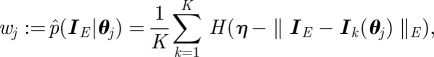
simulations in the η-ball region around the data, with H(x) being the Heaviside step function. This gives an estimate of the time-local likelihood function ; hence, for and ,

4.4

giving the weights of particles for the particle filter (figure 10).

Figure 10.

Comparison of the first six months of data with simulations (a) time series and (b) cumulative distribution of distances.

We use particles, original parameter set , with simulations each, distances dist :=. Still we have some fluctuations without changing the parameters yet (figure 10).

As the next step, we impose a variation in the parameters given by a Gaussian distribution. We vary seasonality θ by 10 per cent with a Gaussian distribution

4.5

with , the original value used for the data simulation, and , which acts like a Gaussian prior, for particles, with simulations each. Most distances are larger than in figure 10, but some are even smaller now (figure 11).

Figure 11.

Comparison of the first six months of data with simulations (a) time series and (b) cumulative distribution of distances, now for varying parameters, here the seasonality.

In the same way, we can vary several parameters and initial conditions, we vary seasonality θ, import ln(ϱ) and initial conditions and , all Gaussian, with the same order of magnitude, and still find distances in the same region as before. As an aside, varying the number of initial susceptibles by 10 per cent changes the simulation trajectories a lot, since owing to conservation of the host population, , a small change in S means a huge change in R. For construction of priors, one should always bear in mind such side effects of dependencies as the one just mentioned.

Now the weight of particle from estimating the time-local likelihood function for dynamic noise is given by

and we perform filtering in the form of sequential importance resampling [32,33] proportional to the weights of particles after each six-month time slice, using an η-ball size of (figure 12).

Figure 12.

(a) Initial distribution versus and (b) final distribution of the seasonality parameter θ after filtering.

4.4. Particle filter in action

Now going times through the time series with each time slice of six months and starting the parameter values not at but at , and not at but at , we find parameters converging to the expected values as shown in the following.

One extra step has to be performed once we go several times through the data time series. The initial variance of the parameters and the initial conditions are decreased by the so-called simulated annealing parameters and at each m-tour an initial variance factor , which are essentially scaling factors for the variance in the Gaussian priors; for details, see Breto et al. [19]. We use, as the update rule with the sample mean over particles at each time slice, the simplest version

4.6

which turns out to perform best, whereas suggested gradient-like update rules seem only to perform well very close to the final estimates, and otherwise receive rather destructive kicks at the main convergence region towards the best estimates. For the results after five times, see figure 13.

Figure 13.

Results for time slice 39 of the last m-run through the data time series for runs. (a) Cumulative distribution for stochastic realizations for each of the now particles and η-ball size of . (b) Fluctuations around the data points originated from the particles. Simultaneous variation of parameters and initial conditions: two model parameters, ln(ϱ), the logarithm of the import, and θ, the seasonality, are drawn from Gaussian distributions with the mean of the original values and standard deviation of 10% of the mean values. Also the two initial conditions I₀ (by 10%) and R₀ are varied. (c) Local likelihood estimate, i.e. the weight of each particle, for the particle parameter values θ. (d) Local likelihood estimate for ln(ϱ).

This shows the qualitative behaviour of the algorithm well, especially indicating that the import parameter is rather more difficult to estimate than the seasonality (figure 13c,d).

Now going times through the time series and more particles, better η resolution gives the results shown in figures 14 and 15. The effect of the simulated annealing is clearly visible, with smaller variation in subsequent m-runs showing up in the estimates. Surprisingly, the import parameter is now also very well estimated after the additional effort of longer filtering.

Figure 14.

Estimates of the parameters along the runs through the time series with now time slices covered, (a) for parameter θ and (b) for ln(ϱ). The update rule for the parameters from one to the next m-run is via simple averaging over the local ℓ-slices, giving numerically more robust results than the gradient update described in Breto et al. [18] and He et al. [19]. But this simple update rule is also advised by Breto et al. [18] and He et al. [19] for the initial phase of convergence. From the initial guesses of the parameters and , the estimates go quickly towards the true parameter values and then perform a random walk around these values, narrowing somewhat in the later m-runs owing to the simulated annealing, i.e. decreasing variance in the variation of particles from one step to the next.

Figure 15.

Two-parameter plot of the best estimates along the run, showing a rapid convergence towards the final parameter region of interest. Initial parameter values are and .

When comparing the simulations of the best estimates with the final piece of time series, the predictive power is quite good in the sense that the simulations now are very close to the data (figure 16).

Figure 16.

The predictive power of the best estimate is visible when comparing the simulations with the original dataset for the last available half year of the time series.

5. Conclusions and discussion

We presented the framework of parameter estimation in simple and in complex dynamical models in population biology, with special emphasis on epidemiological applications. Dynamic population noise, as opposed to observation noise, can be used to construct analytical likelihood functions in simple models and also be estimated via simulations in more complex and more realistic models. Especially in models, which show in its mean field approximation already deterministic chaos it is demonstrated to be possible to estimate well so difficult parameters like the import rate. Future research will now be possible to reinvestigate realistic systems such as dengue fever with very good datasets from Thailand, where import already has been identified as one of the key parameters to determine the underlying dynamical structure of the process.

The presented method of filtering is also close to some elements of approximate Bayesian computations (ABCs), especially the aspect of a distance measure between data and simulations [34,35], and, very recently, ABC methods have been applied to some examples from physics and immune signalling displaying deterministically chaotic behaviour [36]. For the selection between different possible models, see Stollenwerk et al. [37] for an application in an ecological case study, and for a recent application to the paradigmatic Nicholson's blowfly system, an ecological example with chaotic or near chaotic dynamics, see Wood [38]. In the present context, for example, one could see if the available time-series data can distinguish between a four-strain dengue fever model and a simpler model distinguishing only primary and secondary infection and eventually select one and reject the other (which is not always possible given a certain dataset; see Stollenwerk et al. [37]). For an initial study of qualitative similarities and differences in terms of dynamical complexity of such models, see Aguiar et al. [39]. The large number of initial conditions might prohibit the more complex four-strain model from being sufficiently better than the primary versus secondary infection model. Another future research question will be the comparison of spatial stochastic simulations with data, where shifts in epidemiological thresholds are to be expected [40]. Finally, such epidemiological models might help to guide vaccination policies [41], once the dynamical parameters are sufficiently well known to obtain information on the relevant dynamic scenario behind the epidemiological fluctuations.

References

- 1.van Kampen N. G. 1992. Stochastic processes in physics and chemistry. Amsterdam, The Netherlands: North-Holland [Google Scholar]
- 2.Gardiner C. W. 1985. Handbook of stochastic methods. New York, NY: Springer [Google Scholar]
- 3.Stollenwerk N., Jansen V. 2011. Population biology and criticality: from critical birth–death processes to self-organized criticality in mutation pathogen systems. London, UK: Imperial College Press [Google Scholar]
- 4.van Noort S., Stollenwerk N. 2008. From dynamical processes to likelihood functions: an epidemiological application to influenza. In Proc. 8th Conf. on Computational and Mathematical Methods in Science and Engineering, CMMSE 2008, Murcia, Spain, 13–16 June 2008, pp. 651–661 [Google Scholar]
- 5.Aguiar M., Kooi B., Stollenwerk N. 2008. Epidemiology of dengue fever: a model with temporary cross-immunity and possible secondary infection shows bifurcations and chaotic behaviour in wide parameter regions. Math. Model. Nat. Phenom. 3, 48–70 10.1051/mmnp:2008070 (doi:10.1051/mmnp:2008070) [DOI] [Google Scholar]
- 6.Stollenwerk N., Briggs K. M. 2000. Master equation solution of a plant disease model. Phys. Lett. A 274, 84–91 10.1016/S0375-9601(00)00520-X (doi:10.1016/S0375-9601(00)00520-X) [DOI] [Google Scholar]
- 7.Aguiar M., Ballesteros S., Kooi B. W., Stollenwerk N. 2011. The role of seasonality and import in a minimalistic multi-strain dengue model capturing differences between primary and secondary infections: complex dynamics and its implications for data analysis. J. Theoret. Biol. 86, 181–196 10.1016/j.jtbi.2011.08.043 (doi:10.1016/j.jtbi.2011.08.043). [DOI] [PubMed] [Google Scholar]
- 8.Aguiar M., Stollenwerk N., Kooi B. 2009. Torus bifurcations, isolas and chaotic attractors in a simple dengue fever model with ADE and temporary cross immunity. Int. J. Comput. Math. 86, 1867–1877 10.1080/00207160902783532 (doi:10.1080/00207160902783532) [DOI] [Google Scholar]
- 9.Ruelle D. 1989. Chaotic evolution and strange attractors. Cambridge, UK: Cambridge University Press [Google Scholar]
- 10.Ott E. 2002. Chaos in dynamical systems. Cambridge, UK: Cambridge University Press [Google Scholar]
- 11.Kuznetsov Y. A. 2004. Elements of applied bifurcation theory, 3rd edn Applied Mathematical Sciences, no. 112 New York, NY: Springer [Google Scholar]
- 12.Stollenwerk N., Martins J., Pinto A. 2007. The phase transition lines in pair approximation for the basic reinfection model SIRI. Phys. Lett. A 371, 379–388 10.1016/j.physleta.2007.06.040 (doi:10.1016/j.physleta.2007.06.040) [DOI] [Google Scholar]
- 13.Martins J., Aguiar M., Pinto A., Stollenwerk N. 2011. On the series expansion of the spatial SIS evolution operator. J. Diff. Equ. Appl. 17, 1107–1118 10.1080/10236190903153884 (doi:10.1080/10236190903153884) [DOI] [Google Scholar]
- 14.Ballesteros S., Stone L., Camacho A., Vergu E., Cazelles B. Submitted. Fundamental irregularity of regular recurrent influenza epidemics: from theory to observation. [Google Scholar]
- 15.Aguiar M., Stollenwerk N. 2010. Dynamic noise and its role in understanding epidemiological processes. In Proc. ICNAAM, Numerical Analysis and Applied Mathematics, Int. Conf. 2010, Rhodes, Greece (eds Simos T. E., Psihoyios G., Tsitouras Ch.). College Park, MD: American Institute of Physics. [Google Scholar]
- 16.Gillespie D. T. 1976. A general method for numerically simulating the stochastic time evolution of coupled chemical reactions. J. Comput. Phys. 22, 403–434 10.1016/0021-9991(76)90041-3 (doi:10.1016/0021-9991(76)90041-3) [DOI] [Google Scholar]
- 17.Gillespie D. T. 1978. Monte Carlo simulation of random walks with residence time dependent transition probability rates. J. Comput. Phys. 28, 395–407 10.1016/0021-9991(78)90060-8 (doi:10.1016/0021-9991(78)90060-8) [DOI] [Google Scholar]
- 18.Ionides E. L., Breto C., King A. A. 2006. Inference for nonlinear dynamical systems. Proc. Natl Acad. Sci. USA 103, 18 438–18 443 10.1073/pnas.063181103 (doi:10.1073/pnas.063181103) [DOI] [PMC free article] [PubMed] [Google Scholar]
- 19.Breto C., He D., Ionides E. L., King A. A. 2009. Time series analysis via mechanistic models. Ann. Appl. Stat. 3, 319–348 10.1214/08-AOAS201 (doi:10.1214/08-AOAS201) [DOI] [Google Scholar]
- 20.He D., Ionides E. L., King A. A. 2010. Plug-and-play inference for disease dynamics: measles in large and small towns as a case study. J. R. Soc. Interface 7, 271–283 10.1098/rsif.2009.0151 (doi:10.1098/rsif.2009.0151) [DOI] [PMC free article] [PubMed] [Google Scholar]
- 21.Ionides E. L., Bhadra A., Atchade Y., King A. A. 2011. Iterated filtering. Ann. Stat. 39, 1776–1802 10.1214/11-AOS886 (doi:10.1214/11-AOS886) [DOI] [Google Scholar]
- 22.Ballesteros S., Aguiar M., Cazelles B., Kooi B. W., Stollenwerk N. Submitted. On the origin of the irregularity of DHF epidemics. [Google Scholar]
- 23.Aguiar M., Kooi B. W., Martins J., Stollenwerk N. Scaling of stochasticity in dengue hemorrhagic fever epidemics. Math. Model. Nat. Phenom. In press. [Google Scholar]
- 24.Stratonovich R. L. 1959. Optimum nonlinear systems which bring about a separation of a signal with constant parameters from noise. Radiofizika 2, 892–901 [Google Scholar]
- 25.Stratonovich R. L. 1959. On the theory of optimal non-linear filtering of random functions. Theory Probab. Appl. 4, 223–225 [Google Scholar]
- 26.Stratonovich R. L. 1960. Application of the Markov processes theory to optimal filtering. Radio Eng. Electron. Phys. 5, 1–19 [Google Scholar]
- 27.Stratonovich R. L. 1960. Conditional Markov processes. Theory Probab. Appl. 5, 156–178 10.1137/1105015 (doi:10.1137/1105015) [DOI] [Google Scholar]
- 28.Kalman R. E. 1960. A new approach to linear filtering and prediction problems. J. Basic Eng. 82, 35–45 10.1115/1.3662552 (doi:10.1115/1.3662552) [DOI] [Google Scholar]
- 29.Kalman R. E., Bucy R. S. 1961. New results in linear filtering and prediction theory. Trans. ASME Ser. D. J. Basic Eng. 83, 95–108 [Google Scholar]
- 30.Doucet A., De Freitas N., Gordon N. J. 2001. Sequential Monte Carlo methods in practice. Heidelberg, Germany: Springer [Google Scholar]
- 31.Doucet A., Godsill S., Andrieu C. 2000. On sequential Monte Carlo sampling methods for Bayesian filtering. Stat. Comput. 10, 197–208 10.1023/A:1008935410038 (doi:10.1023/A:1008935410038) [DOI] [Google Scholar]
- 32.Doucet A., Johansen A. M. 2008. A tutorial on particle filtering and smoothing: fifteen years later. Technical report, Department of Statistics, University of British Columbia, Vancouver, Canada. See http://www.cs.ubc.ca/%7Earnaud/doucet_johansen_tutorialPF.pdf [Google Scholar]
- 33.Chen Z. 2003. Bayesian filtering: from Kalman filters to particle filters, and beyond. See http://citeseerx.ist.psu.edu/viewdoc/download?doi=10.1.1.107.7415&rep=rep1&type=pdf [Google Scholar]
- 34.Toni T., Welch D., Strelkowa N., Ipsen A., Stumpf M. P. H. 2009. Approximate Bayesian computation scheme for parameter inference and model selection in dynamical systems. J. R. Soc. Interface 6, 187–202 10.1098/rsif.2008.0172 (doi:10.1098/rsif.2008.0172) [DOI] [PMC free article] [PubMed] [Google Scholar]
- 35.Toni T., Stumpf M. P. H. 2010. Simulation-based model selection for dynamical systems in systems and population biology. Bioinformatics 26, 104–110 10.1093/bioinformatics/btp619 (doi:10.1093/bioinformatics/btp619) [DOI] [PMC free article] [PubMed] [Google Scholar]
- 36.Silk D., Kirk P. D. W., Barnes C. P., Toni T., Rose A., Moon S., Dallman M. J., Stumpf M. P. H. 2011. Designing attractive models via automated identification of chaotic and oscillatory dynamical regimes. Nat. Commun. 2, 1–6 10.1038/ncomms1496 (doi:10.1038/ncomms1496) [DOI] [PMC free article] [PubMed] [Google Scholar]
- 37.Stollenwerk N., Drepper F., Siegel H. 2001. Testing nonlinear stochastic models on phytoplankton biomass time series. Ecol. Modell. 144, 261–277 10.1016/S0304-3800(01)00377-5 (doi:10.1016/S0304-3800(01)00377-5) [DOI] [Google Scholar]
- 38.Wood S. N. 2010. Statistical inference for noisy nonlinear ecological dynamic systems. Nature 466, 1102–1104 10.1038/nature09319 (doi:10.1038/nature09319) [DOI] [PubMed] [Google Scholar]
- 39.Aguiar M., Stollenwerk N., Kooi B. W. Submitted. Irregularity in dengue fever epidemics: difference between first and secondary infections drives the rich dynamics more than the detailed number of strains. [Google Scholar]
- 40.Stollenwerk N., van Noort S., Martins J., Aguiar M., Hilker F., Pinto A., Gomes G. 2010. A spatially stochastic epidemic model with partial immunization shows in mean field approximation the reinfection threshold. J. Biol. Dyn. 4, 634–649 10.1080/17513758.2010.487159 (doi:10.1080/17513758.2010.487159) [DOI] [PubMed] [Google Scholar]
- 41.Aguiar M., Ballesteros S., Cazeles B., Kooi B. W., Stollenwerk N. Predictability of dengue epidemics: insights from a simple mechanistic model and its implications for vaccination programs. Submitted. [Google Scholar]