Large-scale Biomedical Image Analysis in Grid Environments

Abstract

Digital microscopy scanners are capable of capturing multi-Gigapixel images from single slides, thus producing images of sizes up to several tens of Gigabytes each, and a research study may have hundreds of slides from a specimen. The sheer size of the images and the complexity of image processing operations create roadblocks to effective integration of large-scale imaging data in research. This paper presents the application of a component-based Grid middleware system for processing extremely large images obtained from digital microscopy devices. We have developed parallel, out-of-core techniques for different classes of data processing operations commonly employed on images from confocal microscopy scanners. These techniques are combined into data pre-processing and analysis pipelines using the component-based middleware system. The experimental results show that 1) our implementation achieves good performance and can handle very large (terabyte-scale) datasets on high-performance Grid nodes, consisting of computation and/or storage clusters, and 2) it can take advantage of multiple Grid nodes connected over high-bandwidth wide-area networks by combining task- and data-parallelism.

1 Introduction

Biomedical imaging plays a crucial role in basic research and clinical studies in biomedicine. In recent years, researchers have enjoyed rapid advances in such imaging technologies as magnetic resonance imaging, digital high-power light microscopy, and digital confocal microscopy. Advanced microscopy instruments that are capable of generating high-resolution images are commercially available. Armed with high-resolution and high-throughput scanners and sensors, a researcher can now collect detailed measurements about biological entities rapidly. Information synthesized from such measurements can be used in testing of specific scientific hypotheses, diagnosis of complex diseases, assessment of the effectiveness of treatment regimens, and study of biological processes in vivo. For example, high-resolution images obtained at microscopic scales from pathology slides generate wealth of information about cellular characteristics of organisms. Analysis of such images allows researchers to study a disease at cellular or subcellular levels and can provide biomarkers for disease diagnosis. While the hardware advances enhance our ability to capture cellular characteristics of tissues and organs at high resolution, management and analysis of very large digital microscopy image datasets is a challenging problem. Image processing in general is inherently compute-intensive and requires high-performance computing techniques. Datasets of high resolution biomedical images add to this complexity because of the very large volumes of image data. A single image obtained using current high-end scanners can be up to tens of Gigabytes in size. A study may generate hundreds or thousands of such images, pushing the size of the datasets to tens of Terabytes.

Grid computing provides a framework to address the computational, storage, and information management requirements of large scale applications. The emergence and increasing adoption of Grid computing in science, medicine, and engineering has been propelled by the confluence of several factors. First, storage and computation clusters built from commodity components enable small and large institutions to easily and inexpensively put up high-performance Grid nodes. Such systems provide cost-effective platforms for high-performance Grid analytical services, where multiple back-end cluster nodes can be used in a coordinated way to execute computation or data intensive analysis operations. Second, high-speed wide area networking infrastructure is becoming commonly available. Large scale initiatives such as TeraGrid have been deploying Gigabit networks connecting high-performance Grid nodes. These advances enable more effective coordinated use of compute and storage clusters located at different institutions. Third, there is a growing suite of Grid-enabled middleware systems to support secure access to Grid end-points and to facilitate efficient execution of applications in a Grid environment. These middleware systems include infrastructure for single sign-on and authentication/authorization across multiple sites [14], tools for monitoring and allocation of dynamic resources [14, 36, 13], middleware for large data transfer and replica management [8, 27, 3, 2], Grid-enabled database and metadata management systems [16, 23], and scientific workflow systems [11, 21, 19, 6].

Digital microscopy applications can greatly benefit from high-performance computation and storage resources and from Grid computing technologies. A challenging issue is to develop image analysis support that can take advantage of high-end Grid nodes (i.e., Grid nodes consisting of clusters) and that can enable efficient execution of data processing workflows across heterogeneous Grid nodes. In our earlier work, we developed a component-based framework, called DataCutter [6], to support execution of data intensive workflows in a Grid environment. DataCutter provides a coarse-grained data flow system. It allows combined use of task- and data-parallelism across heterogeneous collections of storage and compute clusters in a local-area or wide-area network. In this work, we develop a distributed implementation of a data processing pipeline for large image datasets obtained from digital confocal microscopes using the DataCutter middleware system. Our implementation enables execution of applications on a parallel storage or compute cluster. We embed parallel computing techniques as part of our distributed framework in order to optimize the execution of each operation within a Grid node. In that respect, our system allows an institution or a research group to set up a high-performance image processing service on a cluster and make it available as a high-performance Grid analytical node. The implementation also facilitates efficient execution of the data processing pipeline across heterogeneous collections of clusters. It employs combined task-and data-parallelism, allowing portions of the pipeline to run on different clusters, while taking advantage of parallel execution within a cluster. The ability to execute the data processing pipeline across multiple clusters can make it possible for collaborating research groups to take advantage of the processing and storage capacity of individual high-performance Grid nodes located at each collaborating institution.

This paper is an extended compendium of our two conference papers [28, 20]. Each of the conference papers focused on a different subsection of the data processing pipeline and handling of very large out-of-core datasets on a homogeneous cluster. In this paper, we present the entire pipeline and examine the performance of the implementation when it is employed in a heterogeneous environment as well as on homogeneous cluster systems. We evaluate the efficiency of our implementation using very large image datasets on two high-performance Grid nodes, located at two institutions (the Biomedical Informatics Department and the Computer Science and Engineering Department at the Ohio State University). Each Grid node consists of a state-of-the-art cluster. The Grid nodes are connected to each other using wide-area Gigabit network connections. We demonstrate the efficacy of our system using image datasets ranging from a few Gigabytes to Terabytes in size¹.

2 Background and Related Work

In this section, we provide a brief overview of imaging with confocal microscope scanners, related work in Grid computing and Grid middleware systems, and the DataCutter framework.

2.1 Digital Confocal Microscopy

An average observation in confocal microscopy may involve the acquisition of digitized image slides of a tissue sample at up to 150X resolution. Each pixel in an image slide has a three-byte RGB color value. Most digital microscopy systems are designed to automate the acquisition of digitized tissue slides at multiple resolutions. At high resolutions, it may not be possible to generate an image of the entire tissue at once, because of the limited field of view of the instrument. In such cases, advanced scanners capture the entire image in a set of smaller subimages, each of which is scanned at that resolution. During image acquisition at the resolution limit of the microscope, the instrument moves the imaging sensor in X and Y directions in fixed steps. At each step, multiple images of the rectangular subregion (e.g., a 256×256 square pixels subregion) under the sensor are captured at different focal lengths (different points in the Z dimension). Each such rectangular image corresponds to a tile in the entire mosaic. The movement of the sensor is such that neighbor tiles in the same focal plane overlap each other to some extent (usually 10% overlap in each dimension) to aid the stitching process. The entire slide is scanned from left to right and top to bottom, starting from the upper left-most corner subregion of the slide. A stitching process may follow the image capture stage to generate a single image at each focal length (Z value).

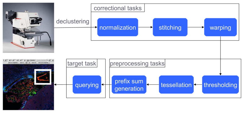
A single slide may produce a multi-Gigabyte image. The data size increases when we factor in the multiple focal lengths at which the slides are acquired. Comparative analyses of different samples could result in multiple Terabytes of image data that need to be stored and processed efficiently. Image analysis operations on these large volumes of data could range from a simple 2D visualization or browsing of the images to more complicated manipulations like 3D reconstruction of the specimen under study from multiple 2D slides. The core data processing steps in the analysis of confocal microscopy images can be summarized in the following main categories: 1) Image Preparation: Stitching, sampling, and re-scaling. 2) Image Correction: Background correction, histogram equalization, normalization. 3) Projection operations: Operations across multiple focal planes. 4) Image Warping: Morphing an image so that it can be “registered” against a standard appearance. 5) Image Segmentation: Edge detection and region extraction operations. 6) Quantitative Image Analysis: Calculation of signal distribution within a sub-region of the image/sub-volume of the stack, pattern/object recognition, and so on. In Section 4, we describe the implementation of a pipeline, consisting of some of these steps, (see Figure 1) using our system.

Figure 1.

Overview of the data processing pipeline targeted in this paper.

Digital microscopy is a relatively new technology. There are a few projects that target creation and management of large microscopy image databases and processing of large microscopy images. The design and implementation of a complete software system was described in [1, 7] that implements a realistic digital emulation of a high power light microscope, through a client/server hardware and software architecture. The implementation emulates the usual behavior of a physical microscope, including continuously moving the stage and changing magnification and focus. The Open Microscopy Environment (http://openmicroscopy.org) project develops a database-driven system for analysis of biological images. The system consists of a relational database that stores image data and metadata. Images in the database can be processed using a series of modular programs. These programs are connected to the back end database; a module in the processing sequence reads its input data from the database and writes its output back to the database so that the next module in the sequence can work on it. While this approach gives a flexible implementation, the back end database can become a performance bottleneck when large volumes of data need to be processed. The Edinburgh Mouse Atlas Project (http://genex.hgu.mrc.ac.uk/) at the University of Edinburgh is developing an atlas of mouse development and database for spatially mapped data such as in situ gene expression and cell lineage. Our work is different in that it targets efficient execution of image processing operations on very large datasets using high-performance Grid nodes.

2.2 Grid and Workflow Middleware Systems

In order to harness the collective power of distributed systems in a Grid environment, an array of tools and frameworks have been developed. These include tools for replica management [8, 27], high speed data transport [4, 2], remote file system access [26], resource monitoring and allocation [36, 14], database and metadata management systems [16, 23], and scientific workflow systems [11, 21, 19, 6]. Grid-computing technologies have been employed in several large-scale projects in biomedicine [25, 5, 22, 31]. Biomedical Informatics Research Network (BIRN) (http://www.nbirn.net) [25] initiative focuses on support for collaborative access to and analysis of datasets generated by neuroimaging studies. MammoGrid [5] is a multi-institutional project funded by the European Union (EU). The objective of this project is to apply Grid middleware and tools to build a distributed database of mammograms and to investigate how it can be used to facilitate collaboration between researchers and clinicians across the EU. eDiamond [31] targets deployment of Grid infrastructure to manage, share, and analyze annotated mammograms captured and stored at multiple sites. One of the goals of MammoGrid and eDiamond is to develop and promote standardization in medical image databases for mammography and other cancer diseases. MEDIGRID [22, 32] is another multi-institutional project investigating the application of Grid technologies for manipulating large medical image databases.

The National Cancer Institute (NCI) funded caBIG (cancer Biomedical Informatics Grid; https://cabig.nci.nih.gov) program is developing a common set of applications, data standards, and a Grid infrastructure to support the data integration and analysis requirements of cancer research projects and facilitate multi-institutional coordinated studies. The caBIG Grid architecture, called caGrid [30], builds on Grid middleware systems such as Globus [14] and Mobius [16] and the Grid Services framework [12, 37]. Using a beta release of caGrid version 1.0, we have developed Grid-enabled applications that provide access to remote computer aided detection algorithms and image data sources as Grid services [24, 29]. The implementation presented in this paper could be wrapped as a Grid service, thus providing access to individual operations and workflows in our implementation through well-defined interfaces. In this work, we focus on the performance aspects of our implementation for processing large image datasets using Grid nodes consisting of storage and compute clusters.

A number of research projects have developed tools and runtime infrastructure to support composition and execution of scientific workflows. The Pegasus project develops systems to support mapping and execution of complex workflows in a Grid environment [11]. The Pegasus framework uses the Condor DAGMan and Condor schedulers [13] for workflow execution. It allows construction of abstract workflows and mappings from abstract workflows to concrete workflows that are executed in the Grid. The Kepler project [21] develops a scientific workflow management system based on the notion of actors. Application components can be expressed as Actors that interact with each other through channels. The actor-oriented approach allows the application developer to reuse components and compose workflows in a hierarchical model. ACDS [19] (Adapting Computational Data Streams) is a framework that addresses construction and adaptation of computational data streams in an application. A computational object performs filtering and data manipulation, and data streams characterize data flow from data servers or from running simulations to the clients of the application.

2.3 DataCutter Middleware System

Our implementation builds on top of DataCutter [6], a component-based middleware framework, which is designed to support efficient execution of data-intensive workflows in a Grid environment. The DataCutter framework provides a coarse-grained data flow system and allows combined use of task- and data-parallelism. In Data-Cutter, application processing structure is implemented as a set of components, referred to as filters, that exchange data through a stream abstraction. A stream denotes a uni-directional data flow from one filter (i.e., the producer) to another (i.e., the consumer). The DataCutter runtime system supports execution of filters on heterogeneous collections of storage and compute clusters in a distributed environment. Multiple copies of a filter can be created and executed, resulting in data parallelism. The runtime system performs all steps necessary to instantiate filters on the desired hosts, to connect all logical endpoints, and to invoke the filter’s processing function. Each filter executes within a separate thread, allowing for CPU, I/O and communication overlap. Data exchange between two filters on the same host is carried out by pointer hand-off operations for languages that support pointers (C++), while message passing is used for communication between filters on different hosts. For this application, we used a version of DataCutter which employs MPI as the message passing substrate. Individual filters may be written in C++, Java or Python, and can be mixed freely within the same workflow.

3 Basic Framework

In this section, we present our basic framework for distributed processing of disk-resident image data. We describe how images are represented and stored. We also present the set of common filters implemented in the system.

3.1 Image Representation

The file representation of microscopy image data has not been standardized. Images are typically stored in universally known formats like JPEG, TIFF, PNG, JPEG2000, as well as proprietary formats used by imaging hardware developers. When image sizes get too large and where the imaging hardware supports it, some file formats, such as Tiled-TIFF and IMG, store the image data as a set of regular rectangular tiles that when “stitched” together appropriately, form the image. In our system, we have designed a representation for the image data, called dim (from Distributed IMage), that seeks to borrow the good features from different existing formats.

In our representation, an image is a raw 3-channel “BGR planar” (Blue-Green-Red planar) image. Each image consists of a set of tiles. The idea of tiling is to enable out-of-core processing of the image data when the image sizes are larger than the memory available on the system. It also enables the distributed storage of the image data across multiple disks and multiple nodes. The tiles are stored in multiple files or multiple contiguous regions of one or more files on disk. A tile represents the unit of I/O. On a cluster system, tiles are declustered across files stored on different compute nodes. A compute node “owns” a particular set of tiles, if the compute node has the tile data available on local disk. A tile contains pixels in a rectangular subregion of the image. It is associated with a bounding box, defined by a [(x_min, y_min), (x_max, y_max)] tuple, in X and Y dimensions of the image and a Z value. The Z value indicates which focal plane (or Z slice) that tile belongs to. The on-disk representation of a tile is one where all the pixels for the B channel are laid out in row major fashion, followed by all pixels for the G channel, and then the R channel. Multiple such images make up a stack. The dim format can be used to represent a stack containing one or more images.

The BGR planar representation also allows us to exploit vector operations on the pixels whenever Intel MMX/SSE instructions are supported. These operations provide low-level parallelism in trivial image processing steps, where the color values of a pixel are modified by some simple function, independent of other pixels. For instance, consider the simple thresholding operation, where each color value of a pixel is set to 1 or 0, depending on whether the original color value for that pixel exceeds or falls below a pre-determined threshold value for that channel. In such a case, we apply the same operation to each color channel, but with different input parameters for different channels. MMX instructions can perform operations on multiple neighboring data at the same time. To benefit from these vector operations, we need to ensure that data (pixels) of the same channel are laid out contiguously. This justifies our use of the BGR planar representation of the image pixel data. However, our framework can be tweaked to support other representations as well.

3.2 Image Declustering

As a precursor to any image processing step, we perform declustering; that is, converting a single large image file into a distributed image file consisting of tiles spread across compute nodes. Certain non-trivial image processing steps may need access to neighbor tiles during execution. In order to minimize inter-processor communication in such steps, the neighbor tiles are grouped to form blocks. A block consists of a subset of tiles that are neighbors in X and Y dimensions of the image and provides a higher-level abstraction for data distribution. All the tiles that have the same bounding box but different Z values are assigned to the same block. In other words, a block is a 3D region covering a subregion in X and Y dimensions and the entire Z dimension in that subregion. A tile is assigned to a single block, and a block is stored on only one node. A node may store multiple blocks. The blocks can be declustered across the nodes in the system according to different configurations like round-robin, stacked, random etc. The user can provide the choice of declustering scheme as input depending on the processing step under question. The user also has a degree of control over the declustering. In addition to providing the set of nodes on the system and the locations on disk where image tiles are to be stored, the user can specify a weight factor to adjust the amount of data assigned to each nodes of the system depending on their relative speeds. In addition to partitioning the image and sending tiles to remote nodes, the declustering produces a .dim file as a final output. This file stores the metadata about each tile that makes up the distributed image. This includes information such as the node where the tile is stored, the location on disk of that tile, the offset within a file where the tile contents are stored, and the resolution of the tile in X and Y dimensions.

3.3 Common Set of Filters

For each step of an application pipeline, we implement application filters that are specific to processing applied in that step. There are also a set of filters that are common to all steps and provide support for reading and writing distributed images. The mediator filter provides a common mechanism to read or write a tile, regardless of whether the target is on local or remote disk. Thus, the location of data is transparent to the application filters, which delegate the I/O requests to mediator filters on the same node. It also provides a means to write out a new tile for an image currently being created, and to finalize all written tiles at once into their final output directories, such that total success or total failure in writing a new image transpires. The mediator filter receives requests from application filters and works with other mediator filters on other nodes to carry out input tile requests. The actual I/O to a local file system is further delegated to a mediator_reader filter, which receives requests from the mediator on the same compute node. The rangefetcher filter is used to hide data retrieval latency. It issues a series of requests on behalf of its application filter to fetch a number of tiles in a sequence. This way, the rangefetcher can work slightly ahead of the application filter, minimizing tile retrieval (either from local disk or from a remote node) latency for the application filter. That is, when an application filter is working on tile T₁, the rangefetcher filter is reading tile T₂, such that when the application needs T₂, it is ready and waiting in memory, reducing read latency.

4 Processing of Confocal Microscopy Images

In this section, we describe our efforts at providing a grid runtime support for executing a pipeline of image processing operations on very large microscopy images. Figure 1 gives an overview of the pipeline starting right from when the images are acquired. The pipeline consists of two main stages; correctional tasks and preprocessing tasks. The final output from this pipeline is a pre-processed processed data that can be queried and analyzed using additional analysis methods. In the following sections we present the implementation of each step using the DataCutter system. Each step is implemented as one or multiple filters. In the implementation, multiple copies of a filter can be instantiated in the environment to process an image in parallel.

4.1 Z Projection Step

The first step in the pipeline is to generate a single image that aggregates all Z planes in the input image. In this process, max aggregate operator is used. That is, each output pixel (x, y) contain the brightest or maximum corresponding input pixel (x, y) value across all Z planes. Since each image blocks contains entire Z dimension for a subregion in X and Y dimension, this stage is pleasingly parallelizable. In other words, each each compute node can independently Z project the data that is assigned to itself without requiring any further communication. In our pipeline one (or more) Z Projection filter per node can be instantiated for this task.

4.2 Normalization Step

During the acquisition of different tiles a variance in illumination may occur. These variances may yield unsightly gradient-like seams in the final output image, and they also hinder efforts at the automatic alignment phase to follow. The goal of the normalization phase is to correct for these variances. This is critical to creating a seamless mosaic of tiles.

The first step in normalization is to compute the average intensity tile for the Z projected plane. The act of computing an average tile for a plane then reinforces what is common across the data and minimizes image specific features thereby giving us an approximation of the illumination gradient. In addition to computing the average tile, an additional offset tile is computed by taking a minimum projection across all the data in the plane. The contributions of the approximated illumination gradient and the pixel offsets to each tile are then removed to give us a corrected dataset. Further details on the normalization technique can be found in [9].

Given a Z plane, the average tile for that plane is one where the pixel value at a position (x, y) within the tile is the average of the pixel values at position (x, y) within all tiles in that plane. Therefore, to compute this average tile, data from the entire Z plane is needed. However, each node owns only a part of the Z projected plane. In our implementation, we have each node initially compute the average tile based on the portions of the Z plane it owns locally. We partition this tile uniformly into P parts, where P is the number of nodes. Then in a ring fashion each node first contributes to an all-to-all reduction operation where starting from their own portion each node sends 1/P-th of the average tile to its neighbor. On receiving a part, each node add its own part to rotating average. At the end of P−1 step each node has the global average for their own part. This operation is followed by an all-to-all broadcast where in a rotating fashion each node’s part is communicated to all processors. After P−1 communication steps, all nodes will have the finalized average tile. This approach requires just 2 × S amount of data transfer. Here, S is the size of the tile. The same procedure is used to compute the offset tile. Using the average and offset tiles, each node then normalizes the portions of the image it owns for each individual Z slice of the original declustered image as well as for the Z projected plane.

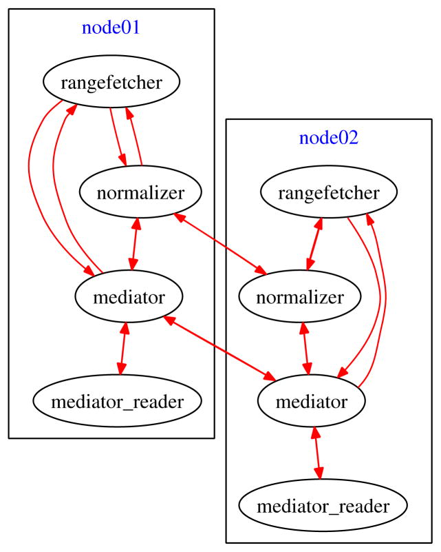
Figure 2 illustrates an example of the DataCutter workflow layout we use for normalization, a typical phase of the larger pipeline. Each oval represents a running filter on a given compute node, and each arrow represents a communication line. Since the normalization is not a compute intensive operation, usually a single normalization filter per compute node would be sufficient along with the help of the mediator to retrieve the data owned by that compute node.

Figure 2.

Low-Level Normalization Workflow

4.3 Automatic Alignment Step

The goal of the automatic alignment phase is to determine how partially overlapping tiles should converge upon one another to produce a properly aligned image, eliminating all the overlapping regions. For an image tiled with c columns and r rows of tiles, one can compute (c−1) × r horizontal alignment displacements, and c × (r−1) vertical alignment displacements. However, only one horizontal and one vertical alignment per tile will suffice to construct an aligned final output image. Consider an undirected graph where each tile is represented as a vertex and each displacement computations (both horizontal and vertical) between its neighbors as an edge. We can generate a spanning tree of the graph, and use this to generate a finalized offsets for each tile. If we use displacement scores as edge weights, a maximum spanning tree of the graph (maximizing the displacement score) will compute the best alignment [9].

When computing the displacement scores for each pair of adjacent tiles, within a single Z plane, horizontal and vertical alignments are processed separately. Each alignment takes two adjacent (overlapping) tiles as input, and performs feature detection without scanning the overlapping region in its entirety. Each tile is filtered with a Sobel filter [15] to compute the gradient of the tile and the highest values from the gradient are then regarded as features. Features are then matched across two adjacent tiles by performing a normalized cross correlation of a window centered on a tile feature from one tile and a region centered on the expected location of the tile feature (found in the first tile) on the other tile. Each horizontal and vertical displacement is given a score. The score used to integrate the horizontal and vertical displacements is the number of feature correspondences found for that particular displacement; the higher the score the better the alignment.

The decomposition of work across compute nodes is as follows. Each compute node is responsible for computing alignments between any tiles it owns and the tiles immediately to the right and below in X and Y dimensions. With a good declustering, most of the time, this means that any pair of alignments require access to two local tiles to compute their alignment. However, on the borders between tiles owned by one compute node and another compute node, some network communication is necessary to process the alignments. When the images are large relative to the number of compute nodes, this border communication cost becomes insignificant. That is, for multi-gigabyte size images, the image dimensions consist of tens of thousand of pixels which is much greater than the number of nodes in a typical cluster. For automatic alignment, one or more alignment filters per compute node can be instantiated (in our experiments we used only one) to compute pairwise alignments. However, only one maximum spanning tree filter will suffice to efficiently compute the spanning tree. When all alignments have been made and scored, the maximum spanning tree filter chooses the best alignments and saves the finalized offsets (into the output image) of every tile to the disk to pass this information to the next phase.

4.4 Stitching Step

The goal of the stitching phase is to produce a final non-overlapping image from the partially overlapping input tiles using the finalized offsets produced by the automatic alignment step. Even though final output image will be smaller than the input image (due to the fact that neighboring tiles in the input will overlap), it will be still extremely large hence the stitching process generates a tiled version of the output image. If the tile sizes are kept “close” to each other in the input and output images, during the stitching process each input tile will contribute (map) to only a small subset of the output tiles. In order to reduce communication between the compute nodes, we preserve as much locality as possible and we generate a “conformal” declustering of output tiles, and a mapping, in such a way that the number of tiles and which compute node they reside on are preserved. We make a one-to-one correspondence between ownership regions in the input and output space, and each compute node is responsible for stitching any tiles it owns in the output space. That is, if a compute node owned the first two rows of tiles in the input space, it would own the first two rows of tiles in the output space. In the majority of cases, the image data in the output space derives from image data in the input space on the same compute node. However, on the borders between tiles owned by one compute node, and another compute node, some network communication will be necessary to merge the final result. Since this operation is I/O intensive due to reading and writing of input and output tiles, a single stitching filter per compute node will be usually sufficient to process data owned by the compute node.

4.5 Warping Step

It is desirable to morph the image to a pre-defined 2D atlas. This provides a mechanism for researchers to compose region-of-interest queries based on a segmentation of the subject under study into regions (e.g., biological regions of a mouse brain) and to compare multiple images or image regions of the same subject type using a common reference. Image warping [35] transforms an image geometrically to conform to a reference geometry. It applies a mapping function, which defines the spatial relationships between pixels in two images. There are two basic types of mapping functions. A forward mapping function maps each input pixel to produce its output pixel location. An inverse mapping function, on the other hand, takes an output pixel location as input and determines which input pixel maps to the output pixel. In the warping step the goal is to compute a mapping function then apply it to the image. Our implementation employs the inverse mapping method, because this method ensures computation of all output pixels and avoids creation of “holes” in the warped image.

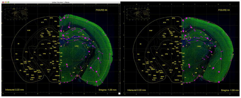
In addition to the input and output images, the image warping operation requires a set of control points as input. The start and end points of each control point correspond to an input pixel location and an output pixel location, respectively. They indicate that the input pixel, marked as the start point of the control point, should be moved to the output pixel, marked as the end point, as the result of the warping operation. A set of control points essentially describes how the input image should be morphed. Figure 3 shows how the control points can be specified to warp an image of a portion of the brain so that it fits a standard brain atlas. On the left we see the unwarped image (colored region) overlay the atlas. On the right, we see the same image warped so as to fit the atlas dimensions.

Figure 3.

Warping of a brain mosaic to a standard brain atlas.

Using the set of control points, the algorithm generates approximate inverse mapping functions that defines the spatial correspondence between two images and are used to produce the set of (p_o, p_i) pairs, where p_o is the output pixel and p_i is the corresponding input pixel that will contribute with minimum error to pixel p_o. The computation of the inverse mapping functions is the first phase of the inverse mapping operation. This phase is referred to as the computation phase. The second phase, which is called mapping, assigns the color values at pixel p_i to p_o, for each input and output pixel. The warping algorithm needs to iterate over the output space and determine which areas of the input space to read from. To determine the inverse mapping transformation (of some order M) for each output pixel, low-order polynomials such as the Weighted Least-Squares with Orthogonal Polynomials (WLOP) technique [35] can be used. The WLOP technique is very compute intensive, but it provides better results than other algorithms by taking pixel - control point locality information into account. We employed the WLOP technique in our implementation. However, our framework allows for a user to plug-in another warping technique.

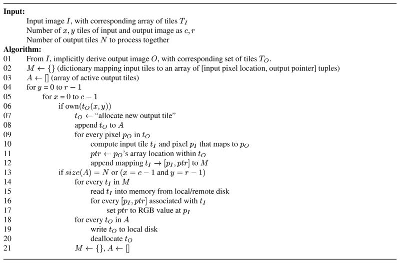
Several researchers have developed algorithms for efficient execution of image warping. Wittenbrink and Somani [34] proposed one of the earliest approaches to address the problem of parallel inverse image warping. They evaluated the algorithm on an SIMD architecture. Contassot-Vivier and Miguet [10] proposed the idea of partitioning an image into sub-regions and then performing warping on these sub-regions in parallel. Their algorithm, however, works only for forward mapping and supports only limited transformations. Jiang et. al. [17] proposed a parallel load-balanced image warping algorithm using forward and inverse mapping that can support many complex warping transformations. We have developed a number of different approaches to support parallel image warping on distributed and disk-resident image data when an inverse mapping function is employed. These approaches include the Serializable Mapping (SM) scheme, the Asymmetric Traveling Salesman Problem Scheduler (ATSP) scheme, and the On-Demand Mapper (ODM) scheme [20]. Unlike the previous work, we have designed and implemented out-of-core algorithms that place minimum restrictions on the size of the images. Our algorithms also work in a completely decentralized fashion. The experimental results show that the ODM approach achieves the best performance on average [20]. In this section we present this approach (Figure 4).

Figure 4.

The On-Demand Mapper (ODM) Algorithm.

In the on-demand mapper approach, the output image is partitioned into tiles and each output tile is assigned to a processor. Each processor works on a subset of output tiles at a time; this subset is referred to as the set of “active” output tiles. This set of tiles is created such that the total size of the active tiles fits in memory. The algorithm fetches input tiles on demand to satisfy the needs of a small set of active output tiles. Each node performs computation on the output tiles that it owns. If a node is an SMP machine, multiple warping filter instances are instantiated on the node; each filter carries out warping computations in parallel on different tiles. Each processor iterates over its output space in some order, one tile after another in the set of active tiles. As soon as it has finished warping a tile, that tile is written to local disk. In this way, each output tile is written exactly once.

Inverse mapping functions for the set of active tiles are computed before any input tiles are retrieved. The algorithm also computes the set of input tiles that will contribute to the pixels in these output tiles. In our system, an input image is partitioned regularly into rectangular tiles. Thus, the complexity of finding the set of input tiles for a given set of output tiles is O(1). Once the set of input tiles have been determined, each input tile is read from local disk or retrieved from the remote processor, on which the input tile is stored. All pixels of the input tile that map to pixels in any of the active output tiles are processed, the pixel values of the corresponding output tiles are updated, and the input tile is evicted from memory. After all the input tiles required for the given set of output tiles have been processed, the output tiles are written to disk. The algorithm moves on to the next set of N active output tiles owned by the node.

The total amount of memory required for the ODM algorithm is equal to the sum of (1) N × S for the output tiles, (2) $N\times S\times \frac{32}{3}$ for the stored mappings and (3) S for the one input tile being read at a time. Here, N is the number of active output tiles and S is the size in bytes of an average tile. The constant $\frac{32}{3}$ is the ratio of the size of the mapping M (see Figure 4) per pixel (32 bytes: 8 bytes for each of the x and y location, 8 bytes for a pointer, and another 8 bytes for the size of a tile) to the size of each pixel (3 bytes for RGB). The ODM algorithm reduces the number of times an input tile must be read. In addition, when handling N output tiles, this algorithm is in effect a perfect scheduler; it schedules all accesses for a given tile such that they all fall sequentially.

4.6. Thresholding Step

The thresholding step generates an output image (of same size with the input image) where every pixel has value of either 0 or 1 depending on whether the color value (RGB: Red, Green, Blue) of the corresponding input pixel is larger than a user-defined threshold or not. A different threshold can be specified for each color (R, G, B). The implementation in our system processes each input tile independently, since there is no dependency between tiles. The naive algorithm to perform the thresholding is to look at every byte one at a time and generate corresponding output pixel value 0 or 1. This can be easily optimized by utilizing vector operations of the current hardware architectures. We have developed an implementation that is based on Intel’s MMX with SSE extensions (which is available on Pentium III and above [18]) and requires a compiler that supports those extensions (e.g., g++ 3.3 or above, or the Intel compiler icc).

In this optimization, the threshold output is computed as out ← min(ones, (t′ − in)). Here in is a sequence of 8 unsigned bytes of an image to be thresholded, and out is the threshold output that will be overwritten with 0 or 1 values at the end of this operation. ones is an array of 8 unsigned bytes filled with the value 1. t is the threshold value (that is, if a byte in in is<= t, it should be set to 1, and to 0 otherwise) and t′ be an array of 8 unsigned bytes filled with the value t+1. Using the Intel MMX/SSE instructions, the threshold operation can be performed in two vector operations. The subtraction operation (t′ − in) uses saturating arithmetic, which means that subtraction overflow sets the result to 0, not a negative number. The following example illustrates the thresholding operation, where t = 5 and in = 1 2 3 4 5 6 7 8:

	t′	6	6	6	6	6	6	6	6
–	in	1	2	3	4	5	6	7	8
		5	4	3	2	1	0	0	0
min	ones	1	1	1	1	1	1	1	1
	out	1	1	1	1	1	0	0	0

4.7. Tessellation Step

The tessellation step reads thresholded pixel data as input and produces tessellation output, which consists of the sum of all nonzero pixels within a user-defined tessellation region. This results in a resolution reduction. The tessellation region is specified by the user in terms of an x and y range, and x × y becomes the factor by which the image resolution is reduced. Even though the output tessellation image is smaller than input thresholded image (by a factor of x × y), the output can still be extremely large; hence the output image is tiled and distributed across storage nodes in the environment.

Between the threshold tiles and the tessellation tiles, we support an arbitrary mapping; i.e., a threshold tile could contribute to multiple tessellation tiles that are assigned to different nodes, and a tessellation tile of a node may need to access tiles from different nodes. This is necessary when the size and number of the threshold tiles do not necessarily correspond to the size and number of the tessellation tiles, and/or when a non-conformal declustering is used for the tessellation image. However, we experimentally evaluated various mappings and observed that by preserving locality (i.e., tessellation tiles only depend on local threshold tiles) one can achieve up to 12x faster execution on a system that uses a switched Gigabit Ethernet network for communication. Therefore, in our implementation we decided to take advantage of this and we only made the size of the tessellation tile a parameter. Furthermore, since we want the tessellation step and the following (co-located) step, the prefix sum, to run in parallel, we actually ensure that each tessellation tile would fit in memory twice, once for the tessellation and once for the prefix sum. The amount of memory to use per node is supplied by the user and for our experiments, we specified this parameter such that we did not exceed the core memory available on each node.

We have also implemented an optimization to speed up the tessellation process that utilizes vector operations. This optimization is similar to those described in Section 4.6, although this time we use a single vector operation (addition).

4.8. Prefix Sum Step

The prefix sum step computes the 2D prefix sum of the values at each point of the tessellated image. The resulting prefix sum values are stored on disk so that aggregation queries can be answered quickly. The 2D prefix sum at each point (x, y) of the tessellated image is given by:

$$\mathit{PSum}(x,y)=\sum _{i=1}^x\sum _{j=1}^y\mathit{value}(i,j)$$ (1)

A 2D prefix sum of a given array can be computed by adding the values sequentially along each dimension of the array. However, since the tessellated image could potentially be too large to fit in memory, a distributed, out-of-core 2D prefix sum algorithm is needed. We have developed two different distributed prefix sum algorithms; full (global) prefix sum and local prefix sum. Both algorithms are implemented as DataCutter filters. During execution multiple instances of filters are created. Each filter instance processes one or more subimages.

The full prefix sum algorithm finalizes the prefix sum across all subimages by the time preprocessing is finished². In doing so, there is an inherent dependency of each prefix sum subimage on the prefix sum subimages to the left of and above it. Thus, a filter handling subimage (x, y) where x > 0 and y > 0, has to wait for values from the filter(s) handling subimages (x−1, y) and (x, y−1). For instance, the filter handling subimage (0,0) finalizes the prefix sum there using an interleaved version of the simple algorithm, and sends its boundary elements i.e. the values in its bottom row to the filter handling subimage (0,1) and the values in its rightmost column to the filter handling subimage (1,0). Since filters can be present on different hosts, this sending of values could involve communication over a network. Filters handling subimages (0,1) and (1,0) include these received values in the computation of their prefix sums so as to produce the finalized prefix sum values at each point in their subimage. These filters then send their appropriate boundary elements to the filters handling subimages to the right of and below their subimage respectively. Thus, a diagonal wave dependency, which moves from left to right along each row and from top to bottom along each column, is introduced in the full prefix sum algorithm. Once a filter has computed the full prefix sum of its subimage and handed off its boundary elements, it writes the prefix sums to disk, frees the memory the subimage occupied, and begins working on another.

The local prefix sum technique eliminates the dependency arising in the full prefix sum computations. In this algorithm, each prefix sum filter instance computes the prefix sum values for the subimages assigned to that filter. After computing the prefix sum values for a subimage, it stores the results on disk. The local prefix sum algorithm allows filters to proceed independently in parallel, since there is no dependency among subimages. However, this improvement in prefix sum generation time comes with a corresponding increase in the complexity of the querying mechanism. The full prefix sums at a query point will now need to be computed on-the-fly by utilizing the local prefix sums of the subimages stored on disk.

4.9. Query Execution

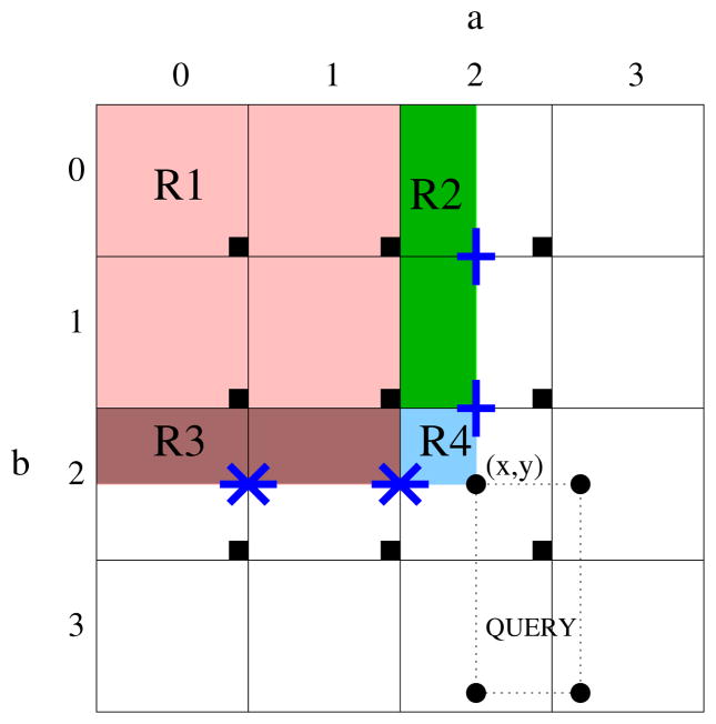
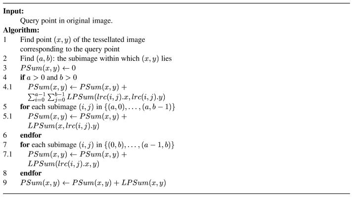
A query in our system is a sequence of points that make up the region of interest within an image. The execution of a query involves the retrieval and computation of the full prefix sum values corresponding to these query points (as a batch). A query client filter identifies for each of the query points the machines on which the prefix sum values are stored. A set of query handler filters are instantiated on each of these hosts. Each handler reads the corresponding prefix sum values from local files. If the prefix sums are generated using the local prefix sum technique, then these represent only the local prefix sums at the points within their respective subimages. The full prefix sum value at each query point must now be computed at runtime, by combining relevant local prefix sum values. Consider a single query point in the original image. Say it corresponds to the point (x, y) in the tessellated image. Let (x, y) lie within subimage (a, b) of the tessellated image as shown in Figure 5.

Figure 5.

Computation of full prefix sum using local prefix sums (with 16 total subimages).

Let PSum(x, y) denote the full prefix sum at (x, y) and LPSum(x, y) denote the local prefix sum at (x, y) within subimage (a,b). The LPSum value at the lower right corner point of any subimage (i, j) will be equal to the sum of all the values within that subimage. These points are denoted as lrc(i, j) and are highlighted in the figure using darkened boxes. lrc(i, j).x and lrc(i, j).y respectively denote the horizontal and vertical coordinates of lrc(i, j) in the image. In other words, lrc(i, j).x gives us the value of the horizontal coordinate for the rightmost column of subimage (i, j) and lrc(i, j).y gives us the vertical coordinate value for the bottom row of (i, j). The algorithm used to compute the full prefix sum at a given query point is shown in Figure 6. The full prefix sum at a point is computed as the aggregate of the local prefix sums within four disjoint regions, numbered from R1 through R4 in Figure 5.

Figure 6.

Algorithm to compute full prefix sum at a point using local prefix sums.

Step 4 of our algorithm is responsible for region R1 of the figure, that is it computes the sum of local prefix sum values at the darkened boxes of each subimage (if there exists any) that completely lie within the rectangular region between point (0,0) and (x, y). As each value represents the sum of all values within their respective subimages, Step 4 effectively computes the sum of values of all points that lie in the region 1, or in other words, the full prefix sum value at lrc(a‒1, b‒1). Steps 5–6 are responsible for region R2 of the figure, that is, they compute the sum of the local prefix sum values at the points that are indicated by “+” symbols in the figure. Thus, they effectively compute the sum of the local prefix sum values of all points within shaded regions of each subimage that lies in the vertical strip between (a,0) and (a, b‒1). Steps 7–8 are responsible for region R3 of the figure, that is, they compute the sum of the local prefix sum values at the points that are indicated by “*” symbols in the figure. Thus, they effectively compute the sum of the local prefix sum values of all points within shaded regions of each subimage that lies in the horizontal strip between (0,b) and (a‒1, b). Step 9 is responsible for region R4 of the figure. By adding the sums computed by each of these steps, we get the sum of the values of all points within the four shaded regions of our figure. In other words, we have the sum of values of all points that lie in the rectangular region [(0,0) − (x, y)]. Thus, at the end of the algorithm, we have effectively computed PSum(x, y), the full prefix sum value at point (x, y).

Once the full prefix sums of all query points are computed, the algorithm described in [33] is used to compute the result of the query.

5 Experimental Results

In this section we present experimental performance evaluation of our implementation. We evaluate the performance under two main configurations: 1) Execution on a single high-performance Grid node, and 2) execution across two Grid nodes.

The largest real image we obtained from a confocal microscope had an uncompressed data size of about 63 Gigabytes. To show scalability in our results, we scaled up these real images by varying factors upto multi-terabyte sized images. We did so by generating replicas of these smaller images, reproducing tiles to the right, below and the lower right (this enabled an easy scale-up by a factor of 4).

We carried out our experiments using a number of different clusters. The first cluster, called OSUMED, consists of 16 nodes. Each node contains one Intel Pentium III 933MHz processor, 512MB of memory and roughly 300GB of locally connected IDE disk, which can sustain a rate of 30MB–40MB per second of read and write transfer. The nodes are connected using a Switched Fast Ethernet network. The second cluster, called XIO, consists of 16 nodes, each node having two Intel Xeon 2.4GHz processors with hyper threading, resulting in 4 virtual CPUs per node. Each node has 4GB of memory and is connected to 7.3TB storage space – each of the 16 nodes mounts an independent 7.3TB ext3 filesystem. We measured the maximum aggregate application-level I/O bandwidth of this cluster as about 2.95 GB/sec. The nodes of the XIO cluster are connected to each other via a switched Gigabit Ethernet network. The third cluster is referred to here as the RII-MEMORY. It consists of 32 dual-processor nodes equipped with 2.4 GHz AMD Opteron processors and 8 GB of memory, interconnected by both an Infiniband and 1Gbps Ethernet network. The storage system consists of 2×250GB SATA disks installed locally on each compute node, joined into a 437GB RAID0 volume with a RAID block size of 256KB. The maximum disk bandwidth available per node is around 35 MB/sec for sequential reads and 55 MB/sec for sequential writes. The fourth cluster, referred to here as RII-COMPUTE, is a heterogeneous 32-node cluster, consisting of a mixture of dual-processor 2.7 GHz AMD Opteron 254 nodes with 4 GB of memory and dual-processor 3.2 GHz Intel Xeon nodes with 2 GB of memory, all interconnected by both and Infiniband and 1Gbps Ethernet network. The RII-MEMORY and RII-COMPUTE clusters are connected through a 10-Gigabit wide-area network connection – each node is connected to the network via a Gigabit card; we observed about 8 Gigabits/sec application level aggregate bandwidth between the two clusters.

5.1 Performance on Single High-performance Grid Nodes

In this section, we present our results from experiments, where each step in the pipeline executes entirely within a single cluster. Also, the image data that the application filters for a step access are also stored on the same cluster. Hence, all data accesses are local to the cluster where the pipeline step is executing. Our results show that our algorithms scale well with the number of processors under the different cluster configurations. The results presented in this section are also available in our conference papers [28, 20].

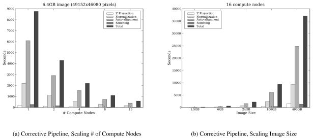
In the first set of experiments, we examined the scalability and relative cost of the z-projection, normalization, autoalignment, and stitching steps. Figure 7(a) presents results obtained on the RII-MEMORY cluster. The pipeline steps are applied to a 6GB input image (49152×46080×1 pixels) as the number of nodes is varied from 1 to 16. The figure shows the relative performance of each step. Autoalignment is the most expensive in all cases. The results show almost linear speedup is achieved in each of these steps. The next set of experiments look at the performance of each step when the size of the dataset is scaled. In Figure 7(b), we apply the same processing steps, using 16 compute nodes, to a 1.5GB, 6GB, 25GB, 100GB and 400GB image. Our results show linear scalability, i.e., the total runtime increases by no more than a factor of 4 when the dataset size is increased by the same amount.

Figure 7.

The execution times of the Z Projection, Normalization, Autoalignment and Stitching steps.

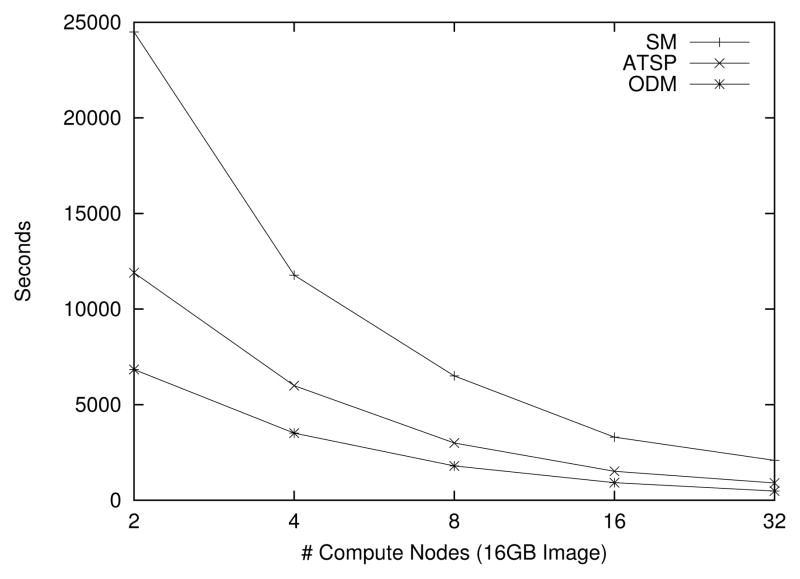
The second set of experiments evaluated the performance of the different algorithms proposed for the parallel execution of the warping step (see Section 4.5). In the experiments, the control points (which define the inverse warping function) were chosen such that the image rotated by 10–20 degrees. In Figure 8, we observe performance implications of increasing the number of compute nodes, acting on an image of size 16GB, for each of the three warping algorithms. As seen from the figure, the implementation achieves close to linear speedup. The ODM algorithm performs best in all cases. This can be attributed to the better I/O performance and lower computational overhead of ODM compared to the other algorithms.

Figure 8.

Varying the number of nodes while the image size is fixed.

To assess the ability of our system in handling very large datasets, we executed the ODM warping algorithm on a 1-Terabyte image. The input image had 690276×534060 pixels, 3 channels, 138 tiles in the x direction, 4416 tiles in the y direction, and 1.73 MB per tile. We used 16 compute nodes. The total time taken was 68830 seconds (about 19 hours). The amount of computation time was equal to 60860 seconds and the I/O time was 7962 seconds (12% of the total execution time). The average number of tiles read per node was 206106, with a standard deviation of 208. Thus, the balance in workload among all compute nodes was quite good, for this experiment.

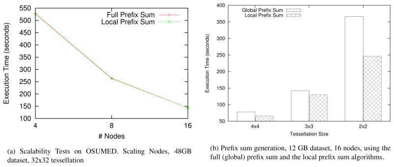
In the third set of experiments, we measured the performance of our algorithms for the prefix sum step. Figure 9(a) shows the performance of the this step as the number of nodes is varied on the OSUMED cluster. In this experiment a square image was partitioned in 48MB files and distributed across the nodes in the system. The user-defined tessellation value was set to 32×32. As seen from the figure, the observed speedup is close to linear as we go from 4 to 16 nodes. We do not observe a substantial difference in running time between the full (global) prefix sum and the local prefix sum. This can be attributed to the fact that the image fits in distributed aggregate memory. As a result, expensive I/O overheads are avoided during the prefix sum step. Figure 9(b) shows the results when the amount of memory is not sufficient to store the data. The total size of the image in this experiment is equal to 12 GB. The image is partitioned across 16 nodes in a round-robin fashion. To simulate the case with limited memory spaca, we allocated only 32MB per node. The user-defined tessellation value was varied between 4×4, 3×3 and 2×2. The performance improvements for the local prefix sum are significant here, since it performs all operations locally.

Figure 9.

Performance of the prefix sum generation step.

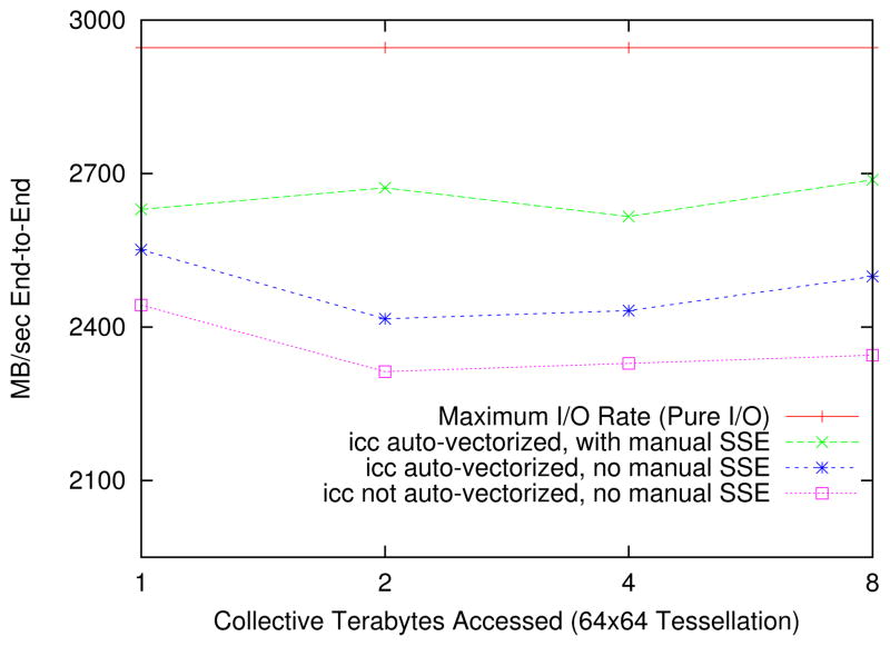
In the last set of experiments, we show that our implementation can achieve close to the application-level maximum raw I/O rate on a state-of-the-art storage cluster. In these experiments, we used the XIO cluster, which is capable of high-performance I/O by modern standards. Our implementation can also take advantage of the low-level vector operations on the CPU. Figure 10 illustrates each of these points. The maximum I/O rate on this cluster was 2.95 GB per second. The maximum rate achieved with the full prefix sum pipeline was 2.68 GB per second, or 91% of the measured maximum I/O rate, on an 8TB original image. This experiment also employs vector operations (known as the SSE instruction set on the Intel architecture).

Figure 10.

XIO Cluster Collective End-to-End Preprocessing Rate (16 nodes, 6GB files)

5.2 Performance Across Grid Nodes

In this set of experiments, we look at the performance of our implementation when the middleware components for a single stage are placed across two Grid nodes. In these experiments, the RII-MEMORY and RII-COMPUTE clusters were used to form the two high-performance Grid nodes. The image data resides on one of the clusters, the RII-MEMORY cluster. However, our application filters for each stage of the pipeline may execute either on the same cluster “local” to the data or on a different “remote” Grid node. In biomedical image analysis application pipelines, have varying computation, memory and storage requirements. When high-bandwidth networks exist between Grid nodes, it may be possible to reduce the overall execution time by executing compute-intensive tasks on the nodes with faster processors, and tasks with high data access requirements on nodes that are close to the data sources.

In the first set of experiments, we show how our framework supports the split execution of a pipeline of imaging operations. That is, we execute certain stages of the pipeline on a cluster that is remote with respect to the location of the data. These experiments were conducted on small-scale data, the aim being to use the trends in the results to justify the idea of split pipeline execution. In these experiments, we partitioned a 5 GB image (15360×14400×8 pixels) dataset across the nodes of RII-MEMORY.

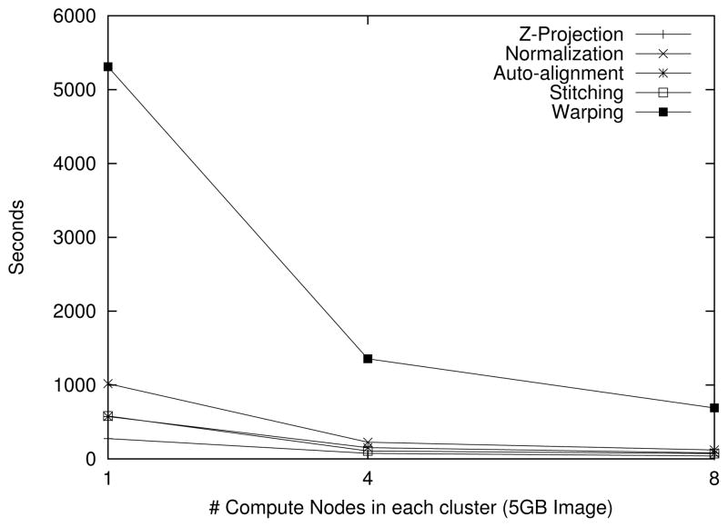
In the first configuration, we placed application filters for each stage of our pipeline on the same nodes of the RII-MEMORY cluster that host the data. In other words, the application filters were placed on the “local” cluster. In the second configuration, we placed application filters on nodes of the “remote” RII-COMPUTE cluster. Our goal is to take advantage of the faster processors and network on the RII-COMPUTE nodes by performing our computations there. The application filters on RII-COMPUTE retrieved data from and write data to the RII-MEMORY nodes over the wide-area Gigabit connection. This is possible on account of the mediator filters that provide transparent data access for the application filters. We placed application filters on the same number of nodes under both configurations. In other words, the second configuration has a one-to-one mapping between the nodes of the two clusters. Even though the filters operate on remote data, Figure 11 shows that we observe linear scalability as we increase the number of nodes.

Figure 11.

Scaling number of compute nodes with remote filter execution.

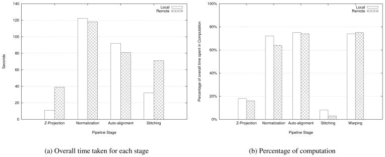
We also compared the performance under the local and remote configurations for a fixed number of nodes. Figure 12(a) shows that the Z-projection and stitching stages of our pipeline execute faster with local application filters, whereas the normalization and alignment stages perform better under the remote configuration. We observed that this trend holds even as the number of nodes is varied. Figure 12(b) shows the percentage of this overall time that is spent purely in the computation phase of the application filters for that stage. From these results, we observe that a stage must necessarily be characterized by a high volume of computation to benefit from remote execution on faster nodes. However, the warping stage performs better under the local configuration despite being a computationally intensive task. This is because the warping stage, unlike normalization and alignment, is also characterized by huge amounts of I/O. We conclude that if an operation in the pipeline performs large amounts of computation relative to the amount of I/O, then the performance of the operation improves if executed remotely on the same number of nodes, but with faster processors.

Figure 12.

Local v/s Remote execution performance (5 GB image, 8 nodes)

This observation directly impacts the performance of our pipeline. We can now split the execution of our pipeline such that the filters for the normalization and alignment stages run remotely while the remaining stages run locally. This way, we can achieve the least turnaround time for each individual stage and hence the best end-to-end performance for the entire pipeline. As an extension to our intelligent filter placement strategy, we can support newer configurations, where the filters on the remote cluster can perform local I/O. For instance, the normalization stage is immediately followed by the autoalignment stage in the pipeline. When both clusters have comparable storage systems, the normalization filters could write their output onto disks local to the remote cluster, so that the autoalignment stage can benefit from local reads.

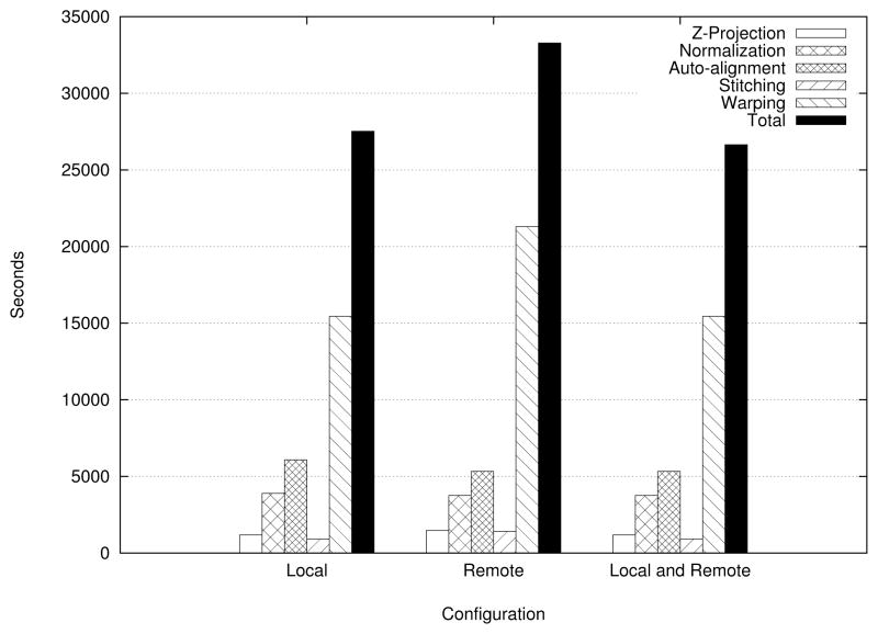
In the second set of experiments, we show the improvement in overall turnaround time for the pipeline, when its execution is performed using multiple Grid nodes. The experiments were conducted with medium-scale data. We partitioned a 256 GB image (159744×197760×3 pixels) dataset across 16 nodes of the RII-MEMORY cluster. The first two set of configurations in Figure 13 show the performance for each stage as well as the total time taken to complete the pipeline under exclusively local and exclusively remote configurations. However, armed with the knowledge about the performances of these stages, we place filters for the normalization and alignment stages on the RII-COMPUTE cluster and the remaining filters on RII-MEMORY and turn our attention to the total time taken to execute the pipeline. The third configuration in the figure represents a hybrid between the exclusively local and remote configurations; in other words, one that is composed of the best configuration for each stage. As we observe from the figure, for this image, the hybrid configuration takes about 26640 seconds and we save 15 minutes by availing of the opportunity to execute pipeline stages across clusters. If we factor in several such images, we end up saving significant amounts of time.

Figure 13.

Execution of pipeline stages across multiple clusters (256 GB image, 32 nodes overall)

In our final experiment, we executed the pipeline on a large image that was 0.5 Terabytes in size. We used 32 nodes each from the RII-MEMORY and RII-COMPUTE clusters. Thus, we have a version of the previous experiment (with 256GB image dataset), where both the image size and the number of nodes have been scaled up by a factor of 2. We used the hybrid configuration for the placement of filters, where the normalize and alignment filters ran remotely. We observed that the total time taken was 30131 seconds, which represents good scalability as compared to the previous experiment (which took 26640 seconds). The difference can be attributed to more data being exchanged over the wide-area and the overhead of extra setup time incurred by doubling the number of nodes.

6 Conclusions

Due to recent advances in hardware technology, biomedical image analysis finds itself at the forefront of many research findings in biomedicine. As image sizes and resolutions grow larger, the researcher can gather lots of information that can give credence to many scientific hypotheses. However, the software technology to support complex analysis of large images either does not exist or is very primitive. In this work, we developed a distributed framework to support execution of complex image analysis operations commonly encountered in digital confocal microscopy. We acknowledge the important role Grids can play in large-scale data analysis, particularly biomedical image analysis. Given that modern-day Grids are composed mainly of well-connected powerful high-end parallel machines, we postulate that a distributed framework for large-scale data analysis must provide high performance within and across these Grid end-nodes. Our framework builds on top of a component-based middleware system and is designed to handle the analysis of terabytes of image data obtained from confocal microscopes. We show that our implementation works across multiple heterogeneous clusters which could be part of different Grid nodes. Our results show that we are able to handle terabyte-sized image datasets and demonstrate good scalability with the size of the images and number of nodes.

References

- 1.Afework A, Beynon MD, Bustamante F, Demarzo A, Ferreira R, Miller R, Silberman M, Saltz J, Sussman A, Tsang H. Digital dynamic telepathology - the Virtual Microscope. Proceedings of the 1998 AMIA Annual Fall Symposium; Nov. 1998; American Medical Informatics Association; [PMC free article] [PubMed] [Google Scholar]
- 2.Allcock B, Bester J, Bresnahan J, Chervenak AL, Foster I, Kesselman C, Meder S, Nefedova V, Quesnal D, Tuecke S. Data management and transfer in high performance computational grid environments. Parallel Computing Journal. 2002 May;28(5):749–771. [Google Scholar]
- 3.Allcock B, Foster I, Nefedova V, Chervenak A, Deelman E, Kesselman C, Lee J, Sim A, Shoshani A, Drach B, Williams D. High-performance remote access to climate simulation data: A challenge problem for data grid technologies. Proceedings of the ACM/IEEE SC1001 Conference; Nov. 2001.ACM Press; [Google Scholar]
- 4.Allcock W, Chervenak A, Foster I, Kesselman C, Salisbury C, Tuecke S. The Data Grid: Towards an architecture for the distributed management and analysis of large scientific datasets. Journal of Network and Computer Applications. 2001;23:187–200. [Google Scholar]
- 5.Amendolia R, Estrella F, Hauer T, Manset D, McCabe D, McClatchey R, Odeh M, Reading T, Rogulin D, Schottlander D, Solomonides T. Grid databases for shared image analysis in the mammogrid project. The Eighth International Database Engineering & Applications Symposium (Ideas’04); July 2004. [Google Scholar]
- 6.Beynon MD, Kurc T, Catalyurek U, Chang C, Sussman A, Saltz J. Distributed processing of very large datasets with DataCutter. Parallel Computing. 2001 Oct;27(11):1457–1478. [Google Scholar]
- 7.Catalyurek U, Beynon MD, Chang C, Kurc T, Sussman A, Saltz J. The virtual microscope. IEEE Transactions on Information Technology in BioMedicine. 2003 Dec;7(4):230–248. doi: 10.1109/titb.2004.823952. [DOI] [PubMed] [Google Scholar]
- 8.Chervenak A, Deelman E, Foster I, Guy L, Hoschek W, Iamnitchi A, Kesselman C, Kunszt P, Ripeanu M, Schwartzkopf B, Stockinger H, Stockinger K, Tierney B. Giggle: a framework for constructing scalable replica location services. Proceedings of the 2002 ACM/IEEE conference on Supercomputing; IEEE Computer Society Press; 2002. pp. 1–17. [Google Scholar]
- 9.Chow SK, Hakozaki H, Price DL, MacLean NAB, Deerinck TJ, Bouwer JC, Martone ME, Peltier ST, Ellisman MH. Automated microscopy system for mosaic acquisition and processing. Journal of Microscopy. 2006 May;222(2):76–84. doi: 10.1111/j.1365-2818.2006.01577.x. [DOI] [PubMed] [Google Scholar]
- 10.Contassot-Vivier S, Miguet S. A load-balanced algorithm for parallel digital image warping. International Journal of Pattern Recognition and Artificial Intelligence. 1999;13(4):445–463. [Google Scholar]
- 11.Deelman E, Blythe J, Gil Y, Kesselman C, Mehta G, Vahi K, Blackburn K, Lazzarini A, Arbree A, Cavanaugh R, Koranda S. Mapping abstract complex workflows onto grid environments. Journal of Grid Computing. 2003;1(1) [Google Scholar]
- 12.Foster I, Kesselman C, Nick J, Tuecke S. Grid services for distributed system integration. IEEE Computer. 2002 June;36(6):37–46. [Google Scholar]
- 13.Frey J, Tannenbaum T, Foster I, Livny M, Tuecke S. Condor-G: A computation management agent for multi-institutional grids. Proceedings of the Tenth IEEE Symposium on High Performance Distributed Computing (HPDC10); IEEE Press; Aug, 2001. [Google Scholar]
- 14.The Globus Project. http://www.globus.org.
- 15.Gonzalez RC, Woods RE. Digital Image Processing. Addison-Wesley Longman Publishing Co., Inc; Boston, MA, USA: 2001. [Google Scholar]
- 16.Hastings S, Langella S, Oster S, Saltz J. Distributed data management and integration: The mobius project. GGF Semantic Grid Workshop; 2004; GGF; Jun, 2004. pp. 20–38. [Google Scholar]
- 17.huang Jiang Y, ming Chang Z, Yang X. A load-balanced parallel algorithm for 2d image warping. In: Cao J, Yang LT, Guo M, Lau FC-M, editors. ISPA, volume 3358 of Lecture Notes in Computer Science. Springer; 2004. pp. 735–745. [Google Scholar]
- 18.Ia-32 intel architecture optimization reference manual. Available at http://www.intel.com/design/pentium4/manuals/248966.htm.
- 19.Isert C, Schwan K. ACDS: Adapting computational data streams for high performance. 14th International Parallel & Distributed Processing Symposium(IPDPS 2000); Cancun, Mexico. May 2000; IEEE Computer Society Press; pp. 641–646. [Google Scholar]
- 20.Kumar V, Rutt B, Kurc T, Catalyurek U, Chow S, Lamont S, Martone M, Saltz J. Large image correction and warping in a cluster environment. Proceedings of Supercomputing 2006 (SC 2006); Tampa, FL. November 2006. [Google Scholar]
- 21.Ludäscher B, Altintas I, Berkley C, Higgins D, Jaeger-Frank E, Jones M, Lee E, Tao J, Zhao Y. Scientific workflow management and the Kepler system. Concurrency and Computation: Practice & Experience, Special Issue on Scientific Workflows, to appear. 2005 [Google Scholar]
- 22.Montagnat J, Breton V, Magnin IE. Using grid technologies to face medical image analysis challenges. BioGrid’03, The 3rd International Symposium on Cluster Computing and the Grid (CCGrid 2003); May 2003.pp. 588–593. [Google Scholar]
- 23.Open Grid Services Architecture Data Access and Integration (OGSA-DAI) doi: 10.1098/rsta.2009.0040. http://www.ogsadai.org.uk. [DOI] [PubMed]
- 24.Pan TC, Gurcan MN, Langella SA, Oster SW, Hastings SL, Sharma A, Rutt BG, Ervin DW, Kurc TM, Siddiqui KM, Saltz JH, Siegel EL. Gridcad: A grid-based computer-aided detection system. Radiographics. 2007 doi: 10.1148/rg.273065153. Accepted for publication, to appear in the July 2007 issue. [DOI] [PubMed] [Google Scholar]
- 25.Peltier S, Ellisman M. The Grid, Blueprint for a New Computing Infrastructure. 2. Elsevier; 2003. The Biomedical Informatics Research Network. [Google Scholar]
- 26.Rajasekar A, Wan M, Moore R. MySRB & SRB - componentsof a data grid. The 11th International Symposium on High Performance Distributed Computing (HPDC-11); July 2002. [Google Scholar]
- 27.Ranganathanand K, Foster I. Identifying dynamic replication strategies for high performance data grids. Proceedings of International Workshop on Grid Computing; Denver, CO. November 2002. [Google Scholar]
- 28.Rutt B, Kumar VS, Pan T, Kurc T, Catalyurek U, Wang Y, Saltz J. Distributed out-of-core preprocessing of very large microscopy images for efficient querying. IEEE International Conference on Cluster Computing; 2005. [Google Scholar]
- 29.Saltz J, Kurc T, Langella S, Hastings S, Oster S, Pan T, Sharma A, Gurcan M. gridimage: Grid computing to middleware support human markup and multiple cad systems. The 92nd Scientific Assembly and Annual Meeting of Radiological Society of North America (RSNA); Chicago, Illinois. November 2006. [Google Scholar]
- 30.Saltz J, Oster S, Hastings S, Langella S, Kurc T, Sanchez W, Kher M, Manisundaram A, Shanbhag K, Covitz P. cagrid: design and implementation of the core architecture of the cancer biomedical informatics grid. Bioinformatics. 2006;22(16):1910–1916. doi: 10.1093/bioinformatics/btl272. [DOI] [PubMed] [Google Scholar]
- 31.Solomonides A, McClatchey R, Odeh M, Brady M, Mulet-Parada M, Schottlander D, Amendolia S. Mammogrid and ediamond: Grids applications in mammogram analysis. Proceedings of the IADIS International Conference: e-Society 2003; 2003. pp. 1032–1033. [Google Scholar]
- 32.Tweed T, Miguet S. Medical image database on the grid: Strategies for data distribution. HealthGrid’03. 2003 Jan;:152–162. [Google Scholar]
- 33.Wang Y, Gupta A, Santini S. Technical report. University of California; San Diego: Dec, 2004. Efficient algorithms for polygonal aggregation queries based on grid tessellations. [Google Scholar]
- 34.Wittenbrink CM, Somani AK. 2d and 3d optimal parallel image warping. International Parallel Processing Symposium; 1993. pp. 331–337. [Google Scholar]
- 35.Wolberg G. Digital Image Warping. IEEE Computer Society Press; Los Alamitos, CA, USA: 1994. [Google Scholar]
- 36.Wolski R, Spring N, Hayes J. The network weather service: A distributed resource performance forecasting service for metacomputing. Journal of Future Generation Computing Systems. 1999;15(5–6):757–768. [Google Scholar]
- 37.Web services resource framework. 2006 http://www.oasis-open.org/committees/wsrf/