Abstract
Segmentation of the left ventricle in MRI images is a task with important diagnostic power. Currently, the evaluation of cardiac function involves the global measurement of volumes and ejection fraction. This evaluation requires the segmentation of the left ventricle contour. In this paper, we propose a new method for automatic detection of the endocardial border in cardiac magnetic resonance images, by using a level set segmentation-based approach. To initialize this level set segmentation algorithm, we propose to threshold the original image and to use the binary image obtained as initial mask for the level set segmentation method. For the localization of the left ventricular cavity, used to pose the initial binary mask, we propose an automatic approach to detect this spatial position by the evaluation of a metric indicating object’s roundness. The segmentation process starts by the initialization of the level set algorithm and ended up through a level set segmentation. The validation process is achieved by comparing the segmentation results, obtained by the automated proposed segmentation process, to manual contours traced by tow experts. The database used was containing one automated and two manual segmentations for each sequence of images. This comparison showed good results with an overall average similarity area of 97.89%.
Keywords: Left ventricle, MRI image, Cardiac function, Contours, Segmentation, Level set
Introduction
Magnetic resonance imaging (MRI) is a noninvasive medical test that helps physicians to diagnose and treat medical conditions. MRI images of the heart are generally clearer and more detailed than some other imaging methods such as X-ray, ultrasound, or computed tomography. This detail makes MRI an invaluable tool in early diagnosis and evaluation of cardiac abnormalities, especially those involving the heart muscle. The left ventricle and in particular the endocardium are a structure of particular interest, since it performs the task of pumping oxygenated blood to the entire body [1]. Therefore, the segmentation of the left ventricle is a task with important diagnostic power. At present, the estimation of the left ventricular (LV) volumes and ejection fraction from cine MR images requires manual tracings of the LV cavity. This manual process introduces considerable latitude for the observer to include varying amounts of endocardial trabeculae and papillary muscles as part of the LV cavity, both at end-diastole as well as end-systole.
This paper is, thus, addressed to the elimination of the observer’s uncertainty. This is achieved by automating the whole segmentation process. We aim to carry out an approximation of the left ventricle’s contours through a level set segmentation algorithm. This algorithm is efficient at finding object edges, from the left ventricle in this case. The major inconvenient of the level set segmentation approach is that the initial points must be introduced manually. In this work, we propose to solve this problem by using an initialization process based on a thresholding operation applied to the original image and, after this, using the obtained binary image as initial mask for the level set method.
The remaining of this paper is organized as follows: We present some related work in left ventricle segmentation in “Related Works in Left Ventricle Segmentation” section. In “Proposed Method” section, we describe and detail the segmentation approach that we propose in this paper. Finally, the database used and the experimental results are given in “Experimental Results” section.
Related Works in Left Ventricle Segmentation
Recently, a number of automatic segmentation algorithms have been developed to detect LV in MRI or echocardiographic images. Some automatic approaches were based on the concept of conserved myocardial volume [2]. In [3], the authors use a complex border detection process, followed by the application of a generalized Hough transform to detect curves and ended up through an active-contour algorithm.
Many algorithms have been proposed for the segmentation of the LV in MRI images. Some methods are based on classification techniques using the grayscale level information [4], in order to segment the endocardium. However, the inclusion of the papillary muscles in the cavity of the mid-ventricular sections remains an open problem [5]. This is due to the fact that the methods using grayscale or gradient information do not make distinction between papillary muscles and myocardium. Indeed, the papillary muscles are areas of low gray level (close to the myocardium intensity), in contrast to the cavity which presents a high gray level value. Furthermore, the methods based on mathematical morphology [6] for segmenting the ventricle reduce the manual intervention but still suffer from parameters adjustment. Some other techniques incorporating prior information in the segmentation process of the left ventricle are also used. A fully automated deformable model technique for myocardium segmentation in 3D MRI technique is presented in [7]. In this work, the authors integrate various sources of prior knowledge learned from annotated image data into a deformable model. Inter-individual shape variation is represented by a statistical point distribution model, and the spatial relationship of the epi- and endocardium is modeled by adapting two coupled triangular surface meshes. To robustly accommodate the variation of gray value appearance around the myocardiac surface, a prior parametric spatially varying feature model is established by using a classification of the gray value surface profiles.
Another automatic atlas-based segmentation algorithm for 4D cardiac MR images is proposed in [8]. This algorithm is based on the 4D extension of the expectation maximization (EM) algorithm. The EM algorithm uses a 4D probabilistic cardiac atlas to estimate the initial model parameters and to integrate prior information into the classification process. The probabilistic cardiac atlas has been constructed from the manual segmentations of 3D cardiac image sequences of 14 subjects. In [9], the authors proposed an improved Markov random field segmentation model, which integrates region prior knowledge and boundary information of the image and this for segmenting LV boundary from cardiac MR image.
The active-contour algorithms are also widely used for the segmentation of cardiac images. However, using these approaches presents some problems associated to the lack of contrast between the myocardium and the cavity, the inclusion of pillars, and the heterogeneity of the cavity due to flow artifacts. On the other hand, the contour initialization is the key to its success. Bad initialization can draw the curve away from the left ventricle to edges that best fit its predefined parameters. To solve this problem, some alternatives approaches have been proposed. As presented in [10], a new approach to magnetic resonance image segmentation with a gradient-vector-flow (GVF)-based approach, applied to selective smoothing filtered images, was developed using non-linear anisotropic diffusion filtering. The system allows automated image segmentation in the presence of gray scale inhomogeneity, as in cardiac magnetic resonance imaging.
Another approach to detect endocardial border on cardiac magnetic resonance images was presented in [11]. This method consists on filtering the short-axis CMR images using connected operators (area-open and area-close filters) to homogenize the cavity, prior to the segmentation which is performed using GVF-snake algorithm.
Proposed Method
In this paper, we propose an automatic method for endocardial border detection using a level set formulation. As mentioned above, the initialization of the active contour and level set algorithms is a very important task. Bad initialization can draw the segmentation resulted curve away from the left ventricle. That is why an automatic initialization is required. To this aim and in order to automate the initialization of the segmentation process, we propose a method based on a thresholding operation of the original image and using the binary image obtained as initial mask for the level set method. This initialization process is based on two steps. First, the image is thresholded using the Otsu filter method. Second, we propose an automatic approach to detect the spatial position corresponding to the region of left ventricular cavity by the evaluation of a metric that indicate object’s roundness. The binary mask is used for initialization of the level set algorithm. For this task, this mask is posed on the circular region detected, in order to initiate the segmentation process.
Initialization with Binary Mask
The method that we propose in this paper is based on the initialization of the level set algorithm by using the binary image obtained from the thresholding operation. For the localization of the left ventricular cavity, we use a method based on the evaluation of a simple metric indicating the roundness of an object because we approximate that the left ventricular cavity has a round shape. To determine if an object is round, we estimate each object area and perimeter and this for all unconnected regions on the image. The metric roundness was defined by the following equation:
 |
1 |
This metric is equal to one only for a circle and is less than one for any other shape.
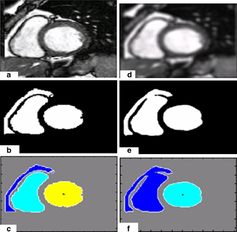
On the short-axis images, the LV endocardial border is not always defined at locations with maximum intensity gradients. That is why we have proposed to smooth the input image with a Gaussian kernel filter to homogenate the LV endocardial border. In Fig. 1, we show an example that illustrates the difference between the left ventricular cavity detected from the original image and from the smoothing image.
Fig. 1.
a A cardiac MR image. b The binary image of the input image. c Labeling of the left ventricular cavity and the other regions. d The input image after smoothing. e The binary image of the smoothing image (Fig. 1d). (f) Labeling of the left ventricular cavity and the other regions
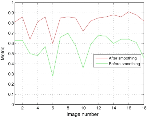
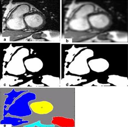
We can clearly notice that the LV metric obtained before smoothing (0.6478) is less than the LV metric obtained after smoothing (0.8638). Figure 2 shows the metric of the LV for 18 images before and after smoothing. The proposed segmentation method in this paper starts by thresholding the input image using OTSU method. After this step, we eliminate the smallest regions (see Fig. 3).
Fig. 2.
The metric evaluated for 18 images before and after smoothing
Fig. 3.
a A cardiac MR image. b The input image after smoothing. c The binary image of the smoothing image. d The binary image after elimination of the smallest regions. f Labeling of the left ventricular cavity and the other regions
Image Segmentation
In image segmentation, the methods based on active contours present dynamic curves that move toward object’s boundaries. To achieve this goal, these approaches explicitly define an external energy that can move the zero-level curve toward the object’s boundaries [12].
For our segmentation process, we propose to use a variational level set formulation of active contours without re-initialization. We describe here this method [12]. Let I be an image and g be the edge indicator function defined by:
 |
2 |
where Gσ is the Gaussian kernel with standard deviation σ. We define an external energy for a function ϕ(x,y) as below:
 |
3 |
where λ > 0 and ν are constants and the terms Lg(ϕ) and Ag(ϕ) are defined by
 |
4 |
And
 |
5 |
where δ is the univariate Dirac function and H is the Heaviside function. Now, we define the following total energy functional
 |
6 |
 |
7 |
The external energy drives the zero-level set toward the object boundaries, while the internal energy μP(ϕ) penalizes the deviation of ϕ from a signed distance function during its evolution. By variations calculating, the gâteaux [13] derivative (first variation) of the functional ε in Eq. 6 can be written as:
 |
8 |
where Δ is the Laplacian operator. Therefore, the function ϕ that minimizes this functional satisfies the Euler–Lagrange equation  . The steepest descent process for minimization of the functional ε is the following gradient flow:
 |
9 |
This gradient flow is the evolution equation of the level set function in the proposed method. The second and the third term in the right-hand side of Eq. 9 correspond to the gradient flows of the energy functional λLg(ϕ) and νAg(ϕ), respectively, and are responsible of driving the zero-level curve toward the object boundaries. To explain the effect of the first term, which is associated to the internal energy μP(ϕ), we notice that the gradient flow Eq. 10 has the factor  as diffusion rate.
 |
10 |
If |Δϕ| >1, the diffusion rate is positive and the effect of this term is the usual diffusion, i.e., making φ more even and therefore reduce the gradient |Δϕ|. If |Δϕ| <1, the term has effect of reverse diffusion and therefore increases the gradient.
Experimental Results
We present here the results given by the implementation of the left ventricular segmentation algorithm proposed in this paper. This segmentation approach is summarized as follows:
First, we threshold the original image by an automatic thresholding algorithm (Otsu algorithm [14]). We obtain a binary image that we use as initial mask for the level set formulation used in our work.
On the second step, we apply the level set algorithm to find the final endocardiel border.
Image Acquisition
For our experiments, we used a free database available for research purposes [15]. The original images in this database consist of short-axis 2D sequences (between eight and 13 sequences of 25 images per patient), with breath-held, ECG-gated acquisitions from base to apex. The most basal slices included in the analysis were located just above mitral valve within LVC. To be included, the basal myocardium had to be visible in the entire circumference at end-systole. The most apical slice was chosen as the one with the smallest visible LVC at end-systole. The sequences were registered on the heart cycle, and thus, they can be stacked to construct 3D sequences. Each 3D sequence is made of 25 volumes and covers a complete heart cycle. A conventional 2D manual segmentation of the LV myocardium was performed by two independent and blinded expert cardiologists. They used a software package that is well established for the post-processing of medical images (Analyze R, Biomedical Imaging Resource, Mayo Clinic Foundation, Rochester, MN, USA). These two experts are called E1 and E2 in the sequel. The cine MR dataset was analyzed as a succession of 2D LV short-axis planes. For each slice location, the experts manually overlaid the endocardial and epicardial contours both at end-diastolic and end-systolic times. During manual tracing, papillary muscles and LV trabeculae were included within the LV myocardium. Then, the segmented slices were stacked to rebuild a 3D object for quantification. The time spent by the experts to manually segment one volume of a 3D + t sequence ranged from 15 to 20 min. For this reason, a manual segmentation is not available at every time-step.
Endocardial Border Detection
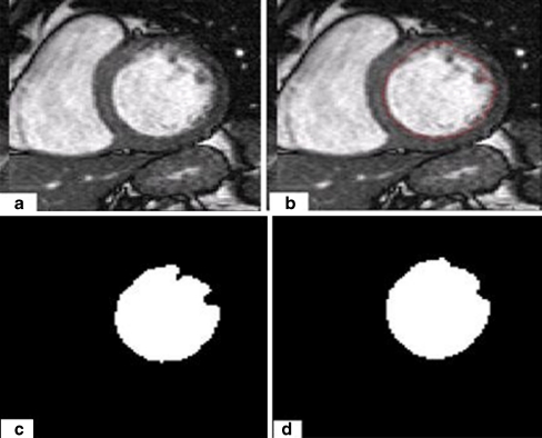
In this section, we present the results of endocardial border detection in cardiac magnetic resonance images using our segmentation approach. The proposed method produces good results, but sometimes some intensity inhomogeneities often occur in left ventricular MRI images and may cause considerable difficulties in image segmentation. As we show in Fig. 4a, heterogeneities in discussion can appear inside of the LVC or be attached with the myocardium muscle. In order to overcome the difficulties caused by intensity heterogeneities, we convoluted the original image with a Gaussian kernel filter. A typical example is given in Fig. 4 with (σ = 1). We notice here that it is necessary to examine the influence of the parameter sigma on the segmentation results.
Fig. 4.
a A cardiac MR image. b Image with final contour. c Segmentation result without convolution. d Segmentation result after convolution
For this purpose, we apply our method using different sigma parameters. The most accurate segmentation result is obtained with the parameter σ = 1.
Evaluation
The segmentation results were evaluated quantitatively using an error metric [16, 17].
 |
11 |
where A is a binary images such all pixels inside the curves produced by a clinical expert and B is the set of all pixels inside the curves produced by a segmentation algorithm.
ε = 3.5: the parameter in the definition of smoothed Dirac function
μ = 0.1: coefficient of the internal (penalizing) energy term P(ϕ)
λ = 1: coefficient of the weighted length term Lg(ϕ)
ν = −0.5: coefficient of the weighted area term Ag(ϕ)
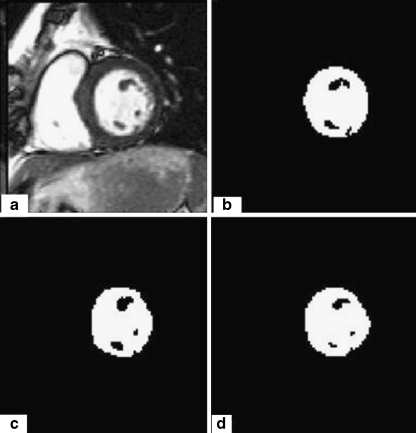
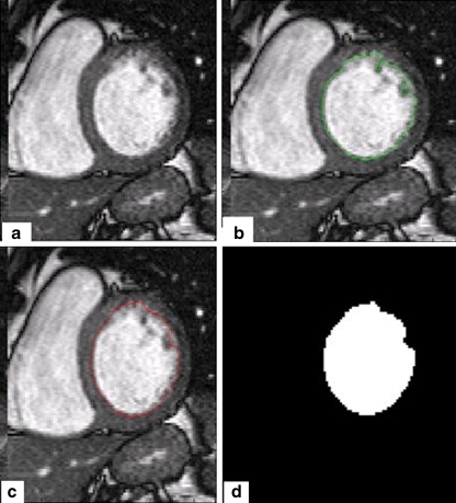
The Fig. 5 shows the results of the two expert segmentation (b and c) and illustrates the method segmentation results (d). The Fig. 6 shows the results of the segmentation method (d) and illustrates the initial and the final contour (the endocardial border) (b and c).
Fig. 5.
a A cardiac MR image. b Segmentation result expert1. c Segmentation result expert2. d Segmentation result proposed method
Fig. 6.
a A cardiac MR image. b Image with initial contour. c Image with final contour. d Segmentation result
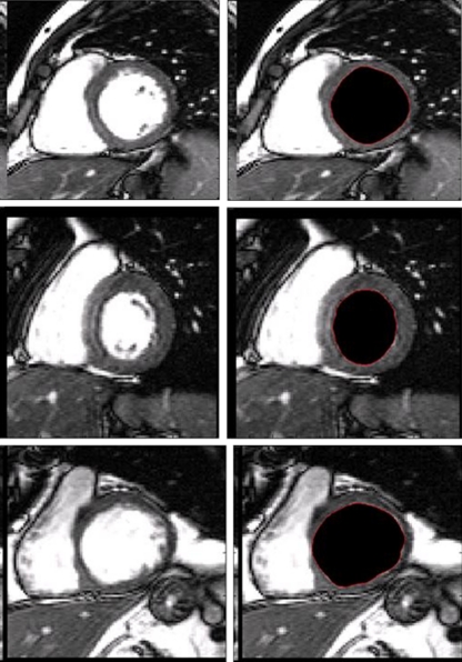
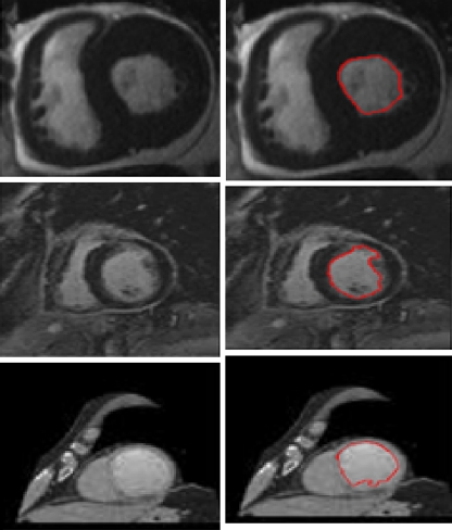
As shown in Fig. 6, the proposed method works efficiently. Others segmentation results are given in Fig. 7.
Fig. 7.
Segmentation results for different MRI images
Table 1 gives the error metric of 18 patient selected from the data bases used in our study. The error metric was evaluated between the proposed method and the two experts (E1 for expert1 and E2 for expert2). As presented in Table 1, we obtained an overall average similarity area of 97.85% (expert1) and 97.89% (expert2).
Table 1.
The error metric for the proposed method at the end-diastole phase
| Patient | E1 (%) | E2 (%) |
|---|---|---|
| PAT01 | 96.31 | 96.65 |
| PAT02 | 99.62 | 96.60 |
| PAT03 | 96.29 | 95.45 |
| PAT04 | 96.46 | 96.82 |
| PAT05 | 93.98 | 98.81 |
| PAT06 | 99.12 | 97.02 |
| PAT07 | 95.44 | 99.65 |
| PAT08 | 99.67 | 99.33 |
| PAT09 | 98.06 | 99.45 |
| PAT10 | 95.04 | 94.86 |
| PAT11 | 98.38 | 99.95 |
| PAT12 | 99.95 | 98.61 |
| PAT13 | 97.87 | 98.51 |
| PAT14 | 98.05 | 97.47 |
| PAT15 | 99.16 | 99.20 |
| PAT16 | 94.51 | 98.94 |
| PAT17 | 98.99 | 98.42 |
| PAT18 | 99.69 | 99.96 |
We have also evaluated this error for the automatic algorithm proposed in [6], where the authors developed an automatic algorithm based on watershed segmentation of 4D cardiac MR images. The automatic segmentation results are available in the database used in this work. Table 2 gives the results of the error metric for the same patients selected in Table 1 at the end-diastole phase for this watershed segmentation algorithm.
Table 2.
The error metric for the watershed algorithm at the end-diastole phase
| Patient | E1 | E2 |
|---|---|---|
| PAT01 | 94.96 | 95.30 |
| PAT02 | 98.72 | 94.94 |
| PAT03 | 88.40 | 96.62 |
| PAT04 | 94.82 | 95.19 |
| PAT05 | 95.02 | 99.85 |
| PAT06 | 98.20 | 99.69 |
| PAT07 | 94.05 | 98.25 |
| PAT08 | 98.64 | 98.98 |
| PAT09 | 96.94 | 98.32 |
| PAT10 | 93.17 | 92.99 |
| PAT11 | 97.04 | 98.70 |
| PAT12 | 96.09 | 97.42 |
| PAT13 | 94.25 | 93.61 |
| PAT14 | 98.16 | 97.36 |
| PAT15 | 97.87 | 99.51 |
| PAT16 | 98.40 | 95.04 |
| PAT17 | 98.91 | 96.33 |
| PAT18 | 93.10 | 93.36 |
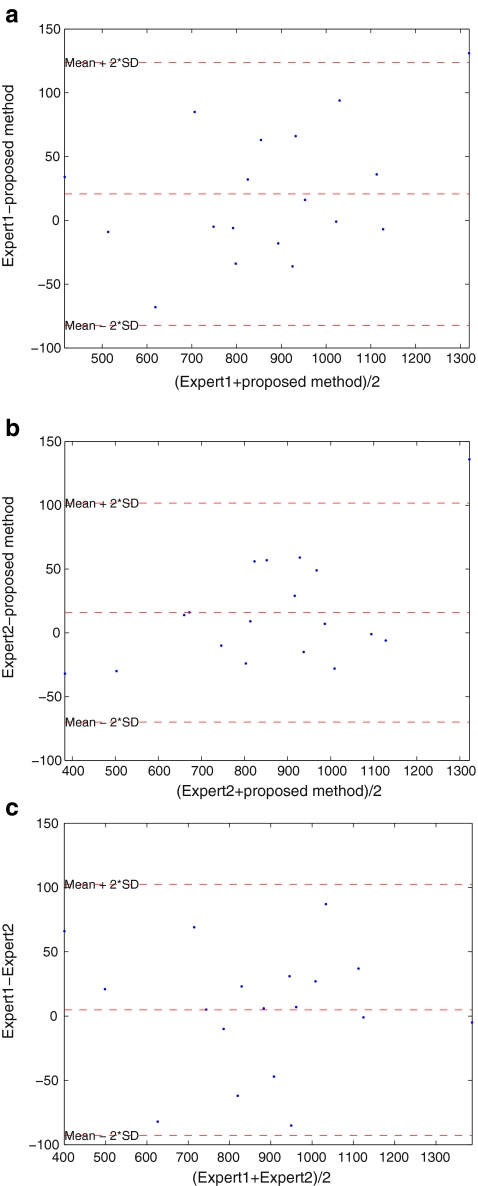
We notice also that we obtained an overall average similarity area of 95.93% (expert1) for the automatic method proposed in [6] (Table 2) and 96.75% for expert2. The agreement between manual and the proposed method was assessed on LV area measures, as reported in Table 1. In order to gain a more meaningful data interpretation, the Bland–Altman [18] plots for the expert1 and the proposed method (Fig. 8a) and the expert2 and the proposed method (Fig. 8b) are shown in Fig. 8.
Fig. 8.
a Bland–Altman plot for expert1 and the proposed method. b Bland–Altman plot for expert2 and the proposed method. c Bland–Altman plot for expert1 and expert2. All area units are in number of pixels
The Bland–Altman plot, or difference plot, is a graphical method used to compare two measurements techniques. In this graphical method, the differences (or alternatively the ratios) between the two techniques are plotted against the averages of the two techniques. Horizontal lines are drawn at the mean difference and at the limits of agreement, which are defined as the mean difference plus and minus 2 times the standard deviation of the differences [19].
We see clearly, from the tow plots, Fig. 8, the agreement between the two experts and the proposed method. This implies that the LV area measured with the new proposed method is in agreement with the LV area obtained with the two experts. The inter-observer variability was shown in Fig. 8c.
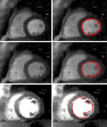
To show the robustness of our method, we illustrate the examples presented in Fig. 9. For all the examples, the inclusion of the left ventricular and the left myocardium and pathologies in the myocardium makes the separation of the two regions using any algorithms very difficult.
Fig. 9.
Segmentation results for different MRI images
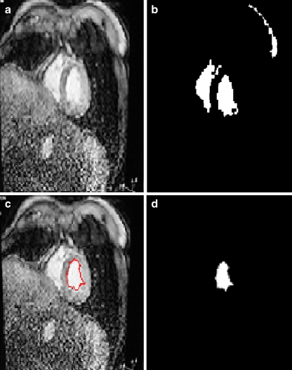
Generally pathologies in the myocardium cause a non-circular shape of the left ventricular. Meanwhile based on the metric used in this work, we can say that left ventricular cavity has the biggest value. For more explication, we illustrate the following example.
As shown in Fig. 10, the result of the thresholding operation shows three regions: in the middle the left (0.46) and the right (0.37) ventricular and the other region (0.13). So we see clearly that the left ventricular have not exactly a circular shape but they have the biggest value.
Fig. 10.
a A cardiac MR image. b Image after thresholding. c Image with final contour. d Segmentation result
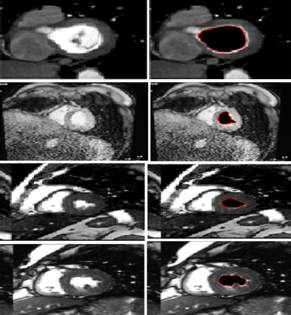
We have test our algorithm using MRI images with contrast enhancement and perfusion. Images were obtained with sequences with considerable less S/N and more inhomogeneities (Figs. 11 and 12). The results shown in Figs. 11 and 12 prove that our algorithm can successfully be implemented with this kind of image.
Fig. 11.
MRI images with contrast enhancement segmentation
Fig. 12.
MRI images perfusion segmentation
Conclusion
This paper describes a new automatic method to detect the left ventricular chamber and the endocardial border in short-axis MRI view. This method takes into account the intensity inhomogeneities which often occur in left ventricular cavity and may cause considerable difficulties in image segmentation. A Gaussian kernel filter has been used to solve this problem. We proposed to threshold the original image, and we used the binary image obtained as initial mask for a level set segmentation method. For the localization of the left ventricular cavity, we use an approach based on the evaluation of a metric that indicate the object’s roundness.
In order to assess our method, an error metric was evaluated between the proposed method and two expert’s manual segmentation (expert1 and expert2) for 18 end-diastole images. The results obtained prove that the proposed approach is very promising. We have obtained a mean of 97.78% for expert1 and 97.89% for expert2. These results are in the most cases more precise than those obtained with another automated segmentation approach presented in Table 2.
Contributor Information
Mohammed Ammar, Email: ammar.mohammed4@gmail.com.
Saïd Mahmoudi, Phone: +32-65-374056, FAX: +32-65-374500, Email: Said.Mahmoudi@umons.ac.be.
Mohammed Amine Chikh, Email: mea.chikh@mail.univ-tlemcen.dz.
Amine Abbou, Email: abbou.amine@yahoo.fr.
References
- 1.Paragios N, Jolly MP, Taron M, Ramaraj R. Active shape models segmentation of the left ventricle in echocardiography. Lecture Notes in Computer Science. 2005;3459:131–142. doi: 10.1007/11408031_12. [DOI] [Google Scholar]
- 2.Garson CD, Li B, Acton ST, Hossack JA. Guiding automated left ventricular chamber segmentation in cardiac imaging using the concept of conserved myocardial volume. Comput Med Imaging Graph. 2008;32:321–330. doi: 10.1016/j.compmedimag.2008.02.004. [DOI] [PMC free article] [PubMed] [Google Scholar]
- 3.Fernandez-Caballero A, Vega-Riesco JM. Determining heart parameters through left ventricular automatic segmentation for heart disease diagnosis. Expert Systems with Applications. 2009;36:2234–2249. doi: 10.1016/j.eswa.2007.12.045. [DOI] [Google Scholar]
- 4.Lynch M, Ghita O, Whelan PF. Automatic segmentation of the left ventricle cavity and myocardium in MRI data. Comput Biol Med. 2006;36(4):389–407. doi: 10.1016/j.compbiomed.2005.01.005. [DOI] [PubMed] [Google Scholar]
- 5.Monitillo A, Metaxas D, Axel L. Automated segmentation of the left and right ventricles in 4D cardiac, SPAMM images. MICCAI, LNCS. 2002;2488:620–633. doi: 10.1007/3-540-45786-0_77. [DOI] [PMC free article] [PubMed] [Google Scholar]
- 6.Cousty J, Najman L, Couprie M, Clément-Guinaudeau S, Goissen T, Garot J: Automated accurate and fast segmentation of 4D cardiac MR image. In: Procs of Functional Imaging an Modeling of the Heart, LNCS 4466, 2007, pp 474–483
- 7.Kausa MR, Berga J, Weesea J, Niessenb W, Pekar V. Automated segmentation of the left ventricle in cardiac MRI. Medical Image Analysis. 2004;8(3):245–254. doi: 10.1016/j.media.2004.06.015. [DOI] [PubMed] [Google Scholar]
- 8.Lorenzo-Valdés M, Sanchez-Ortiz GI, Mohiaddin R, Rueckert D. Segmentation of 4D Cardiac MR Images Using a Probabilistic Atlas and the EM Algorithm. Berlin: Springer; 2003. pp. 440–450. [DOI] [PubMed] [Google Scholar]
- 9.Wang G, Guo Y, Zhangk S, Ma Y: A novel segmentation method for left ventricular from cardiac MR images based on improved Markov random field model. In: Image and Signal Processing, CISP’09, 2009, pp 1–5
- 10.Santarelli MF, Positano V, Michelassi C, Lombardi M, Landini L. Automated cardiac MR image segmentation: theory and measurement evaluation. Medical Engineering Physics. 2003;25:149–159. doi: 10.1016/S1350-4533(02)00144-3. [DOI] [PubMed] [Google Scholar]
- 11.ElBerbari R, Frouin F, Redheuil A, Angelinic E-D, Mousseaux E, Bloch I, Herment A. Development and evaluation of an automatic segmentation method of endocardial border in cardiac magnetic resonance images. ITBM-RBM. 2007;28:117–123. [Google Scholar]
- 12.Li C, Xu C, Gui C, Fox MD: Level set evolution without reinitialization: A new variational formulation. In: Proceedings of CVPR’05 1, 2005, pp 430–436
- 13.Evans L. Partial Differential Equations. Providence: American Mathematical Society; 1998. [Google Scholar]
- 14.Otsu N. A threshold selection method from gray-level histograms. IEEE Trans Syst Man Cybern. 1979;9(1):62–66. doi: 10.1109/TSMC.1979.4310076. [DOI] [Google Scholar]
- 15.Najman L, Cousty J, Couprie M, Talbot H, Guinaudeau S, Goissen T, Garot J: An open, clinically validated database of 3D+t cine-MR images of the left ventricle with associated manual and automated segmentations. In: Insight Journal, 2007 special issue entitled ISC/NA-MIC Workshop on Open Science at MICCAI, 2007
- 16.Hammoude A: Computer-assisted endocardial border identification from a sequence of two-dimensional echocardiographic images. Ph.D. dissertation, Univ. Washington, Seattle, WA, 1988
- 17.Mendonc T, Andre RS, et al: Comparison of segmentation methods for automatic diagnosis of dermoscopy images. In: IEEE EMBS, France, 1-4244-0788-5, 2007 [DOI] [PubMed]
- 18.Altman DG, Bland JM. Measurement in medicine: the analysis of method comparison studies. Statistician. 1983;32:307–317. doi: 10.2307/2987937. [DOI] [Google Scholar]
- 19.Thunberg P, Emilsson K, Rask P, Kähäri A. Separating the left cardiac ventricle from the atrium in short axis MR images using the equation of the atrioventricular plane. Clin Physiol Funct Imaging. 2008;28(4):222–228. doi: 10.1111/j.1475-097X.2008.00799.x. [DOI] [PubMed] [Google Scholar]


