Improving Protein Template Recognition by Using Small-Angle X-Ray Scattering Profiles

Abstract

Small-angle x-ray scattering (SAXS) is able to extract low-resolution protein shape information without requiring a specific crystal formation. However, it has found little use in atomic-level protein structure determination due to the uncertainty of residue-level structural assignment. We developed a new algorithm, SAXSTER, to couple the raw SAXS data with protein-fold-recognition algorithms and thus improve template-based protein-structure predictions. We designed nine different matching scoring functions of template and experimental SAXS profiles. The logarithm of the integrated correlation score showed the best template recognition ability and had the highest correlation with the true template modeling (TM)-score of the target structures. We tested the method in large-scale protein-fold-recognition experiments and achieved significant improvements in prioritizing the best template structures. When SAXSTER was applied to the proteins of asymmetric SAXS profile distributions, the average TM-score of the top-ranking templates increased by 18% after homologous templates were excluded, which corresponds to a p-value < 10⁻⁹ in Student's t-test. These data demonstrate a promising use of SAXS data to facilitate computational protein structure modeling, which is expected to work most efficiently for proteins of irregular global shape and/or multiple-domain protein complexes.

Introduction

Despite the considerable progress that has been made in protein folding and structure prediction, template-based modeling (TBM), which uses experimental structures of homologous proteins to guide the modeling procedure, is still the only reliable method for predicting high-resolution protein structures (1,2). The critical step of TBM is the identification of correct template proteins from the Protein Data Base (PDB) library (3) through a procedure called threading (4,5). The current threading algorithms work well in recognizing templates that have an evolutionary relation to the target proteins. However, for a target lacking homologous templates, the threading algorithms often fail to rank the best alignments to the top, which significantly degrades the power of computer-based protein structure predictions. To overcome this barrier, investigators have developed a variety of methods to exploit the raw experimental data, obtained mainly from x-ray crystallography (6) and NMR spectroscopy (7–9), to assist the computational modeling algorithms for high-resolution structure determination.

Compared with x-ray crystallography, the small-angle x-ray scattering (SAXS) technique is advantageous in that it allows proteins to be studied at near-physiological conditions and does not require crystal formation. SAXS provides low-resolution structural information about many proteins that are recalcitrant to crystallization. Furthermore, in contrast to NMR, it has no macromolecular mass limitation. Nevertheless, SAXS has drawn far less attention in the field of protein structure determination, mainly due to the low resolution of the data (10–50 Å) (10). Unlike x-ray crystallography and NMR data, which specify atomic coordinates, SAXS only provides the shape information of protein molecules in the form of distance histograms without atomic assignment. Furthermore, it lacks a standard SAXS metric in the distance profile assessment and comparison, which could be most sensitively used for atomic-structure determination.

In this work, we explore the possibility of combining SAXS data with computational protein structure prediction, thereby improving the ranking and selection of templates generated by threading algorithms, the most critical step of TBM structure prediction. This issue was partially addressed by Zheng and Doniach (11), who used SAXS data to filter templates generated by gapless threading. Because the optimal query-template alignments will almost always have gaps/insertions, the gapless threading data cannot be used for the real process of protein structure prediction. Here, we developed a new algorithm called SAXSTER (Fig. 1) to systematically examine the sensitivity of various SAXS metrics to template ranking and selection. We used query-template alignments generated by one of the state-of-the-art threading algorithms, MUSTER (12), although the algorithm can be applied to alignments generated by any other programs. We focused mainly on difficult protein targets that lack homologous templates in the PDB library. The SAXSTER server and programs are freely available at http://zhanglab.ccmb.med.umich.edu/SAXSTER.

Figure 1.

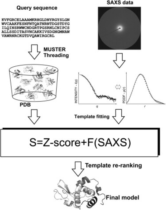
Flow chart of SAXSTER, combining SAXS data and MUSTER for protein structure prediction.

Materials and Methods

Data set

To train and test the SAXSTER algorithm, we collected a list of nonhomologous proteins from PISCES (13), using a sequence identity cutoff of 30%, sequence length of 50–1000 AA, R-factor < 0.15, and resolution better than 1.5 Å. We first selected 200 structures to derive the effective scattering factors for coarse-grained (CG) SAXS simulation, and 341 proteins (201 easy and 140 hard, according to MUSTER) to train the SAXSTER energy function. Another set with 412 structures (232 easy and 180 hard) was used as the test set for the algorithms. To further test the hypothesis that SAXS information should be the most sensitive for proteins of elongated topology, we selected entries from the remaining protein list that satisfied two criteria: 1), a SAXS pair distance distribution function (PDDF) peak that is at most 20% of the maximum pairwise distance; and 2), a MUSTER Z-score < 7.5. This included 141 proteins that constituted our second test set of proteins. In addition, we collected a set of five proteins for which SAXS experimental data are available to validate our CG model and to test the SAXSTER procedure for a real case of SAXS data.

Outline of the SAXSTER protocol

The SAXS-assisted MUSTER fold-recognition algorithm, SAXSTER, consists of five steps: threading-based template identification, full-length model construction, CG SAXS profile calculation, SAXS data matching, and template re-ranking. The inputs of SAXSTER include the amino acid sequence of the target proteins and SAXS data (either the intensity profile in reciprocal space or the PDDF in real space), with outputs being the template structures and the query-template alignments (see Fig. 1).

Threading-based template identification

For a given query protein, we used MUSTER (12) to thread the sequence through a nonredundant set of proteins collected from the PDB, with the purpose of identifying template proteins having similar structure to the query. The scoring function of aligning the ith residue of the query and the jth residue of the template is given by

$$\text{S}\left(i,j\right)=\sum _{k=1}^{20}\left(P{c}_q\left(i,k\right)+P{d}_q\left(i,k\right)\right)L_t\left(j,k\right)/2+c_1\delta \left(s_q\left(i\right),s_t\left(j\right)\right)+c_2\sum _{k=1}^{20}P{s}_t\left(j,k\right)L_q\left(i,k\right)+c_3\left(1-2|S{A}_q\left(i\right)-S{A}_t\left(j\right)\right)+{\text{c}}_4(1-2|{\varphi }_q\left(i\right)-{\varphi }_t\left(j\right))+c_5(1-2|{\phi }_q\left(i\right)-{\phi }_t\left(j\right)|){+\text{c}}_{6}M\left(A{A}_q\left(i\right),A{A}_t\left(j\right)\right)+c_7,$$ (1)

where q is the query and t is the template. The first term in Eq. 1 represents the sequence-derived profiles, where Pc_q(i, k) is the frequency of the kth amino acid at the ith position of the multiple sequence alignment by PSI-BLAST at an E-value cutoff of 0.001, Pd_q(i, k) is the remote homology frequency matrix by PSI-BLAST with E < 1.0, and L_t(j, k) is the log-odds profile of the template. The second term denotes the secondary structure match, and δ(s_q(i), s_t(j)) = 1 when the secondary structures of i and j are the same, and −1 when they are different. The third term counts for the depth of the aligned residues, where Ps_t(j, k) is the depth-dependent structure profile and L_q(i, k) is the log-odds profile of the query. The fourth, fifth, and sixth terms compute the match between the solvent accessibility, ϕ angle, and ψ angle of the query and template, respectively. The seventh term counts the hydrophobic match of the residues based on the hydrophobic scoring matrix. The last parameter of c₇ is introduced to avoid the alignment of unrelated residues in the local regions. The best tuning parameters are c₁ = 0.66, c₂ = 0.39, c₃ = 1.60, c₄ = 0.19, c₅ = 0.19, c₆ = 0.31, c₇ = 0.99, g_o = 7.01, and g_e = 0.55, which we obtained by maximizing the average template modeling (TM)-score of 111 training proteins. All of the nine parameters were searched through a nine-dimensional lattice system (12). Parameters c_1–7 are the weighting parameters in Eq. 1, and g_o and g_e are gap-opening and gap-extension penalties, respectively, in dynamic programming.

For each template, only the best alignment is selected by the Needleman-Wunsch dynamic programming. The templates are then ranked by Z-score:

$$Z-\text{score}=\frac{S-\langle S\rangle }{\sqrt{\langle S^2\rangle -{\langle S\rangle }^2}},$$ (2)

where $S=1/N_{ali}{\sum }_{i=1}^{N_{ali}}S\left(i,i\right)$ is the sum of raw scores from N_ali aligned residue pairs. Based on our benchmarking test, when Z-score > 7.5, 98% of the templates will have a correct fold with TM-score > 0.5, and when Z-score < 7.5, only 5.3% of the templates will do so. Therefore, we define the proteins with a template of Z-score > 7.5 as easy targets, and those with Z-score < 7.5 as hard targets. The MUSTER program and the database can be freely downloaded at http://zhanglab.ccmb.med.umich.edu/MUSTER/.

Full-length model construction from threading alignments

Threading models almost always contain gaps or insertions. Because SAXS data are usually obtained from full-length models, to extract the appropriate SAXS profile from templates, we tried three different methods to quickly construct the full-length C_α trace models. In the first approach, the aligned residues are first copied from the template and kept frozen. The structures in the unaligned regions are built by a self-avoided random walk of C_α-C_α bond vectors of fixed length 3.8 Å starting from the N-terminal of each gap. During the random walk, any walk with a distance to other nonneighboring C_α atoms < 3.8 Å will be discarded. Virtual C_α(i-1)-C_α(i)-C_α(i+1) bond angles are restricted in the range of 65°–165°. To guide the random walk toward its end point, only walks with l < 3.54n are allowed at each step (where l is the distance between the current C_α and the first C_α of the next template fragment, and n is the number of remaining C_α-C_α bonds in the walk). For a template gap that is too big to span by a specified number of unaligned residues, the aligned residues in both sides of the gap will be gradually released until l < 3.54n is satisfied before the random walk starts. Detailed discussions about the sensitivity of the calculated SAXS profile to the gap size by random walk are given in the Supporting Material.

The second method uses MODELLER (14) to build full-length models from threading alignments. From a given query-template alignment, we ran MODELLER using the automodel class in the standard mode. Because MODELLER constructs models by optimally satisfying the spatial restraints from the alignment, MODELLER models are usually very close to the template structure but with loops filled.

The third approach uses the loop/tail modeling component of I-TASSER (15,16), which keeps the threading aligned structure frozen. It was run on a single replica with 200 sweeps, which took <1 min for most of the test proteins.

SAXS profile construction and comparison

SAXS profile calculations from atomic protein structures

For a given protein structure model, we simulate the SAXS intensity profile according to Debye's equation:

$$I\left(q\right)=\sum _{i=1}^{N+W}\sum _{j=1}^{N+W}{f}_i\left(q\right)f_j\left(q\right)\frac{\sin \left(q{d}_{ij}\right)}{q{d}_{ij}},$$ (3)

where q = (4π sinθ)/λ is the scattering vector in Å⁻¹ units sampled up to q_max= 0.50 Å⁻¹ in the bin size of Δq = 0.01 Å⁻¹; λ is the x-ray wave length; 2θ is the scattering angle; N is the number of atoms of the model; W is the number of “dummy” water molecules around the protein representing the hydration shell; d_ij is the distance between atoms i and j; and f(q) is the atomic scattering factor, which depends on the specific atoms (H, C, N, O and S). All hydrogen atoms are taken implicitly and their positions are assumed to be in the correspondent heavy atom coordinates that are covalently bonded. The term for the contribution of the solvent to the scattering pattern is added in the scattering factor (17):

$$f_i\left(q\right)=f_i^{vac}\left(q\right)-{\rho }_{bulk}{V}_i\exp \left(-\frac{V_i^{2/3}}{4\pi }{q}^2\right),$$ (4)

where $f_i^{vac}\left(q\right)$ is the vacuum contribution of atom i taken from the International Tables for Crystallography (18), and ρ_bulk is the electronic density of the bulk water at 20°C (its value is fixed in our simulation by ρ_bulk = 0.334 e⁻Å⁻³). The excluded volume V_i by the ith atom or atomic group (CH, CH₂, CH₃, NH, NH_2, NH₃, and SH) is taken from previous experimental values (17,19).

Furthermore, our calculation includes an explicit model with W water molecules around the protein molecule with a hydration shell ∼3 Å thickness (20). To take into account these water molecules in our model, we started from a face-centered cubic (FCC) lattice system with edge length L_cell, where each point in the lattice represents a dummy molecule consisting of one oxygen and two hydrogen atoms. Its atomic scattering factor comes from the vacuum contribution of those two elements. The protein structure is then projected onto the FCC system and only dummy waters in the range of 3.5–6.5 Å to any C_α atoms are kept. The only free parameter in this model is the density of the lattice represented in terms of L_cell, the edge of the unit cell in the FCC lattice, which can be represented by the contrast of hydration shell (δρ) as follows:

The density of points N_FCC in the FCC lattice with volume V_FCC is defined by

$${\rho }_{FCC}=\frac{N_{FCC}}{V_{FCC}}=\frac{4k^3}{L^3},$$ (5)

where k = 1,2,3, … is the number of unit cells in the x, y, z directions, and L = k × L_cell is the maximum length for each direction. Because the FCC lattice has four effective points per cell (eight on the cube corner contributing one-eighth of its volume plus six in the middle of every face contributing one-half of its volume), each cell contains four dummy waters or equivalently 40 electrons. Hence, the number of excess electrons per volume in the hydration shell relative to the bulk water is given by

$$\delta \rho =\frac{40\text{electrons}}{L_{cell}^3}={\rho }_{\text{shell}}-{\rho }_{bulk}.$$ (6)

The PDDF is calculated from the atomic coordinates of the protein structure plus dummy water molecules by (21,22):

$$p\left(r\right)=\sum _{i=1}^{N+W}\sum _{j=1}^{N+W}{f}_i\left(q=0\right)f_j\left(q=0\right)\delta \left(r-d_{ij}\right),$$ (7)

where δ (r) is the Dirac function. We use a sampling grid on r with step 1 Å. It is expected that p(r) will be a smooth function (23), but in some cases we find a slightly oscillatory pattern that comes from treating coordinates of atoms as single points without any dimension. To overcome this problem, we smooth p(r) using the same algorithm used in the GASBOR real-space version (21).

SAXS profile calculations from C_α-trace models

Because our threading-based models are composed solely of α carbons, we extend the CG model of Yang et al. (24) to calculate the SAXS profiles from the C_α traces:

$$\{\begin{array}{l}I\left(q\right)=\sum _{i=1}^{N+W}\sum _{j=1}^{N+W}{f}_{eff}^i\left(q\right)f_{eff}^j\left(q\right)\frac{\sin \left(q{d}_{ij}\right)}{q{d}_{ij}}\hfill \\ p\left(r\right)=\sum _{i=1}^{N+W}\sum _{j=1}^{N+W}{f}_{eff}^i\left(q=0\right)f_{eff}^j\left(q=0\right)\delta \left(r-d_{ij}\right)\hfill \end{array},$$ (8)

where d_ij is the distance between the ith and jth components of the system (C_α or H₂O), N is the total number of residues in the protein chain, and W is the number of dummy waters around it. In contrast to Yang et al.'s model, however, our hydration shell representation contains dummy waters arranged in an FCC lattice where the number of water molecules is adjusted to mimic the density contrast effect. Consecutively, this approximation is faster than Yang et al.'s approach because it uses fewer water molecules rather than considering several dummy molecules around the protein taken from an equilibrated bulk solvent (water box). Thus, the FCC approach is faster without compromising accuracy. For instance, from our experimental target set composed of five proteins, we have <χ²>_FCC = 0.62, whereas <χ²>_{water box} = 0.59, which is essentially the same result. Furthermore, our CG model represents the pairwise distribution of the protein in real space in addition to the intensity profile, which makes the approach more flexible for many applications.

In Eq. 8, f_eff (q) is the effective scattering factor:

$$f_{eff}\left(q\right)={\langle \sum _{i=1}^n\sum _{j=1}^n{f}_i\left(q\right)f_j\left(q\right)\frac{\sin \left(q{d}_{ij}\right)}{q{d}_{ij}}\rangle }^{1/2},$$ (9)

where 〈···〉 denotes the average over all residues of the same type calculated from 200 randomly selected high-resolution PDB structures, n is the number of atoms for a given residue type, and the term f(q) in Eq. 9 is calculated by means of Eq. 4. As a result, we have 20 effective scattering factors for each amino acid type. In the case of dummy water, its effective scattering factor is calculated by Eq. 9 with n = 3, d_ij = 0, with f_i(q) being the vacuum scattering factors for either hydrogen or oxygen.

SAXS data fitting

We calculated the SAXS profiles for the templates using the CG model from full-length models built by random walk, MODELLER, or I-TASSER as described above. The literature (20) suggests a density of the hydration shell (ρ_shell) 10% higher than the density of the bulk solvent (ρ_bulk). For 20°C, ρ_bulk = 0.334 e⁻Å⁻³ and ρ_shell = 1.10 × ρ_bulk = 0.367e⁻Å⁻³. Then, the density contrast δρ = ρ_shell − ρ_bulk∼0.03. A plain grid search to the density contrast δρ in the range of [0.00–0.03] in step 0.005e⁻Å⁻³ was carried out for each template model to minimize the scoring functions according to this free parameter.

The density contrast δρ in Fig. 2 was adjusted to fit the experimental profile by the CG model with δρ in the range of [0.00–0.05]. The fitting in reciprocal space was made by minimizing the profile matching function I in Table S1 using I_j(q) = kI_j^CG(q), where k is a scaling factor. In real space, we used function IX in Table S1.

Figure 2.

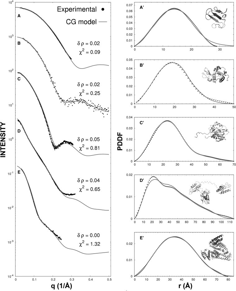
Comparison of the experimental SAXS profiles with those obtained by the CG model in both reciprocal (left) and real (right) spaces. (A and A′) PF1282 P. furiosus, with SAXS data and structural model taken from the BIOISIS databank (BIOISIS ID: 1RBDGP). (B and B′) Lysozyme, with SAXS data from CRYSOL and structure model from the PDB (PDB ID: 6LYZ). (C and C′) PF1528 P. furiosus, with SAXS data and structural model from BIOISIS (BIOISIS ID: 1AMIGP). (D and D′) U2AF65 Splicing factor, with SAXS data and structural model from BIOISIS (BIOISIS ID: 1U2FKP). (E and E′) HSA, with SAXS data from our unpublished data and structure from a homologous protein in the PDB (PDB ID: 1AO6A).

In principle, small δρ produces large unit cells (L_cell) through Eq. 6, and the SAXS profiles would depend on the orientation of the protein structure in the lattice. The lowest nonzero level of δρ is 0.005 and it leads to a lattice of parameter L_cell = 20 Å, which has a nearest-neighbor distance $d_0=L_{cell}/\sqrt{2}$ ∼14 Å. The next level of δρ = 0.010 leads to d₁ ∼ 11.2 Å. On the other hand, the resolution limit of SAXS (d) data can be approximated by d ∼ 2π/q_max, where q_max is the maximum scattering vector of the SAXS profile. Then for q_max = 0.50 Å⁻¹, the resolution limit d = 12.6 Å ∼ d₀ > d₁, and therefore the orientation of the protein in this FCC lattice has minor importance for the SAXS profile calculations.

Ab initio and template-based protein shape restoration

We generated ab initio envelopes from experimental curves using DAMMIF (25), imposing neither point-group symmetry nor anisometry. The template-based method selects the top hit from all nonhomologous structures available in the template library by using the CG model according to the scoring function F_SAXS = log (1 − corr (p_temp (r), p_SAXS (r))), where corr is given by Eq. 11 below. The top template structure was filled by a distribution of points of an FCC lattice to approximately represent the volume of the target protein. Finally, all structures were superposed onto each other through SUPCOMB (26). For easy visualization, surfaces for both DAMMIF and template-based envelopes were calculated using NCSMASK (27).

SAXS-assisted template prioritization

Scoring function

For each target, MUSTER generates alignment of the sequence to 40,096 different templates in the library. To improve the selection of template alignments, we combine the threading Z-score and the SAXS data as follows:

$$S_{comb}\left(i,j\right)=Z_{MUSTER}\left(i,j\right)+w{F}_{SAXS}\left(i,j\right),$$ (10)

where i and j correspond to the query and template structures, respectively; Z_MUSTER(i, j) is the Z-score of the threading alignment; F_SAXS(i, j) is the SAXS profile match of the query and template structures, which can take any scoring format in Table S1; and w is the weighting parameter to balance the threading score and SAXS data.

In Table S1, the Pearson correlation coefficient (PCC) between the template and SAXS profiles is defined as

$$corr\left[p{}_{temp}\left(r\right),p_{saxs}\left(r\right)\right]=\frac{{\sum }_{i=1}^m\left(p_{temp}\left(r_i\right)-\langle p_{temp}\left(r\right)\rangle \right)\left(p_{saxs}\left(r_i\right)-\langle p_{saxs}\left(r\right)\rangle \right)}{\sqrt{{\sum }_{j=1}^m{\left(p_{temp}\left(r_j\right)-\langle p_{temp}\left(r\right)\rangle \right)}^2}\sqrt{{\sum }_{i=1}^m{\left(p_{saxs}\left(r_i\right)-\langle p_{saxs}\left(r\right)\rangle \right)}^2}},$$ (11)

where the sum runs through m evenly distributed positions in the r space. The correlation in q space can be written similarly.

Parameter training

To determine the weighting parameter in Eq. 10, we selected 341 nonredundant training proteins (201 easy and 140 hard) with the alignments to templates generated by MUSTER. The value of w is determined by minimizing the linear regression of TM-score and S_comb:

$$G=\sum _{i=1}^{341}\sum _{j=1}^{N_{temp}}\left\{g\left(TM\left(i,j\right)\right)-S_{comb}\left(i,j\right)+b\left(i\right)\right\},$$ (12)

where the g function is in a sigmoid form:

$$g\left(TM\left(i,j\right)\right)=\frac{k_1}{1+\exp \left[k_2\left(TM\left(i,j\right)-k_3\right)\right]}+k_4,$$ (13)

with k₁ = 9.0, k₂ = 30.0, k₃ = 0.30 and k₄ = 1.0 decided by trial and error in the training process. Because most of the good templates are found in the top 100 templates according to the raw score of MUSTER alignment, we only trained Eq. 12 with N_temp = 100.

We trained our data using all nine different F_SAXS scoring functions. We obtained the best result from F_SAXS = log{1 − corr (p_i (r), p_j (r))}with the weight parameter w = 0.809.

Results

Validation of the CG SAXS model

Because threading-based models contain only Cα conformations, we used an extended CG model to simulate the SAXS data from the C_α traces (see Eq. 8). Other programs, such as CRYSOL (19) and FoXS (28), calculate the SAXS intensity curve I(q) from full-atomic protein structures, and two free parameters are used to fit the simulated curves with the experimental SAXS intensity. In our CG approximation, we need only one parameter, the number of excess electrons δρ (see Eq. 6), to adjust the density contrast of the hydration shell.

Fig. 2 shows a comparison between the experimental data and the simulated curves obtained by the CG model in both reciprocal and real spaces for the five proteins for which SAXS data are available. The experimental PDDF was obtained by GNOM (29), which makes an indirect Fourier transform from the experimental intensity profile I(q). For the CG model, we derived the intensities and PDDFs using Eq. 8. All p(r) values were normalized to unit, and I(q) profiles were plotted in the relative scale. The values of the fitting parameter δρ and the χ² of the fittings, $1/n{\sum }_{k=1}^n{\left(I_{CG}\left(q_k\right)-I\left(q_k\right)\right)}^2/{\sigma }^2\left(q_k\right)$, were attached in each plot, where n is the number of scattering vectors collected from experiments, I_CG(q_k) and I(q_k) are respectively the CG-model derived and experimental values of the intensities of kth vector q, and σ(q_k) is the experimental error of I(q_k).

Overall, there is a good agreement between the experimental and theoretical curves produced by the CG model, with an average χ² = 0.624, indicating that the differences of the curve and data are mainly within the experimental errors. Generally, the CG model fits slightly better to the SAXS data for the proteins with experimentally solved structures than for the proteins that have structures from homologous proteins or were generated by homology modeling. For instance, Fig. 2, C and C′, show the SAXS profiles for the PF1528 Pyrococcus furiosus with SAXS data from the BIOISIS databank, where the structure was generated by homologous modeling (30). The uncertainty of the long tail at the N-terminus has a major impact on the mismatch of the theoretical and experimental profiles (χ² = 0.81). The structures in Fig. 2, D and E, are both multiple-domain structures. The structure of U2AF65 Splicing factor in Fig. 2 D was obtained from the assembly of three domains from other homologous proteins, and the structure of human serum albumin (HSA) in Fig. 2 E was obtained from a homologous protein 1AO6A. The uncertainty of the domain orientations in these two examples contributes mainly to the slightly higher mismatch, with χ² = 0.65 and 1.32, respectively.

Lysozyme is often used as the gold standard for calibration and validation of SAXS simulations (19,21,22,24), partly because both the high-resolution PDB structures and SAXS data are available in the databases. The χ² of the intensities is 0.252 by our CG model (Fig. 2 B). We also calculated the profiles using CRYSOL (version 2.6) and FoXS (version 2010), both of which are based on atomic-structure models. The χ²-values for CRYSOL and FoXS are 0.203 and 0.202, respectively, and thus are slightly lower than that of the CG models. Nevertheless, these data confirm that the CG model, which is based on the C_α-trace only and obtained with a single fitting parameter, can generate a sufficiently accurate fit to the experiments that is well below the typical experimental error.

Shape reconstruction by CG SAXS fitting

As the first implementation of the CG model for protein template identification, we examined the ability of the SAXS-based score to reconstruct a 3D protein shape from 1D SAXS pattern data. Here, neither threading alignment information nor homologous template structures to the target sequence were taken into account. We carried out the shape reconstruction process by matching the simulated PDDF profiles from template protein structures in the nonredundant PDB library with the experimental SAXS profile, p(r), for each of the five target proteins in Fig. 2. We then reconstructed the target protein shape from the first template protein that had the highest profile correlation score (see Materials and Methods).

Fig. S1 shows a comparison between the low-resolution envelopes obtained by DAMMIF (25) and that obtained by our simple template match method. Despite the simplicity of the method, it successfully reconstructed the target protein shapes, which are in a close agreement with those obtained from the sophisticated ab initio restoring programs.

Nevertheless, one cannot expect a simple shape match to recognize the correct topology of the protein structure, since multiple arrangements of secondary structure elements may result in a similar shape but completely different topologies. In fact, the template proteins with the best SAXS profile matches have only an average TM-score of ∼0.3 in structural alignment, which is close to the random similarity in the topology level, whereas the best template recognized by the threading program MUSTER (12) has a TM-score of 0.51 for the same set of proteins.

Nevertheless, the encouraging results for shape reconstruction suggest that the CG model can be combined with other protein-structure prediction techniques (e.g., fold-recognition methods) to filter out incorrect templates that have shape mismatches with the SAXS data.

Selection of the SAXS profile matching score

One can use a number of different ways to compare the SAXS profiles of two protein structures. Here, we evaluated the performance of nine different SAXS-profile matching scores with regard to their ability to recognize the best protein structure templates, as shown in Table S1.

We first measured the PCC between the TM-score of the template structure and the SAXS profile matching scoring function. As an example, Fig. S2, A and C, show the data for the TM-score versus the Z-score of the SAXS matching score for a particular target protein (1IC2A) using two different SAXS-based scoring functions from Schemes I and IX in Table S1. Although both scoring functions could recognize good templates (TM-score ≥ 0.5) as having higher score values, the data distribution from Scheme IX had an obviously higher overall correlation coefficient (i.e., the PCC for Scheme I was 0.19, whereas that for Scheme IX was 0.35). In Fig. S2, B and D, we show the TM-score values of the templates versus a combination of the SAXS-profile matching score and the Z-score of MUSTER threading alignment (see Eq. 10) from the two scoring schemes. After the scores are combined, two distributions have a similar correlation coefficient (∼0.73). However, only the scoring function of Scheme IX improved the original top template selected by MUSTER and increased the TM-score from 0.49 to 0.81.

To summarize the results, Table S1 shows the average PCC and TM-score of selected templates calculated from 341 target proteins. Column 3 presents the results of PCC obtained using only the SAXS profile matching score, and columns 4–6 show results obtained using the combined score of SAXS data match and MUSTER Z-score. The optimal weights of the combination were determined by training in a similar fashion for each case (see Materials and Methods). Overall, the average PCC for SAXS scores was ∼0.36. When combined with the MUSTER Z-score, the SAXS-based scores VIII and IX have an obviously higher PCC value than the other scores. Although the average TM-scores of the first and the best in the top five are all higher than those of the original MUSTER program, the best performance comes from Scheme IX in regard to the average TM-score of the templates. These data suggest that despite the subtle differences among the SAXS-based scores, they have different influences on fold recognition, and certain scoring functions can be more efficient than others.

Function IX in Table S1, in the form of F_SAXS = log{1 − corr (p_i (r), p_j (r))}, was finally selected based on the correlation and TM-score data in our training proteins. This functional form has three main features that contribute to its somewhat advanced performance. First, it does not depend on any scaling factor between the target and template SAXS profiles. Second, its log function encompassing the entire function enhances subtle numerical differences in the score among top templates (see, e.g., Fig. S2 C), thereby facilitating the training process for accurate weighting. Third, it is based on real space, which may undergo less influence through the CG model whose derivation does not taken into account any excluded volume correction, which may be more important in reciprocal space.

Results for proteins with SAXS experimental data

Before executing a large-scale test, we applied the SAXSTER method to the five target proteins for which experimental SAXS data are available (see Fig. 2). Here, we used the combined scoring function of the MUSTER Z-score and the SAXS profile (Eq. 10), where F_SAXS is based on p(r) in Scheme IX of Table S1 as previously mentioned. The alignment gaps in the template structures were filled by random walks. All homologous templates with a sequence identity >30% to the target protein were excluded in the test.

For the HSA protein, the MUSTER Z-score can rank the best alignment of the library at the top, and there is no room for improvement of this target by alignment re-ranking. For two other cases (6LYZ and 1U2FKP), the SAXS score was not sensitive enough to recognize better templates. Although no improvement was demonstrated for these three cases, we found that SAXSTER selects templates that are the same as the top templates selected by MUSTER.

SAXSTER outperformed the MUSTER template selections for an easy and a hard protein. For the easy target, 1AMIGP, the TM-scores of the top template selected by SAXSTER and MUSTER were 0.73 0.68, respectively. For the hard target, 1RBDGP, the SAXSTER algorithm increased the TM-score of the top template from 0.35 to 0.42. Generally, the SAXS score is less sensitive to proteins with a globular shape. However, in this hard target, which has a globular shape (Fig. 2 A′), MUSTER originally ranked the wrong template with an elongated shape that was filtered by the SAXS profile data, resulting in the TM-score improvement.

Results from a large-scale test of template recognition

We tested SAXSTER on 412 target proteins randomly selected by PISCES, which included 232 easy and 180 hard cases according to the MUSTER categorization. In Table 1 we compare the TM-scores of the templates selected by the original MUSTER Z-score and the SAXSTER scores. For SAXSTER, we tried the schemes F_SAXS= log{1 − corr (I_i (r), I_j (r))} for reciprocal space (SAXSTER I(q)) and F_SAXS= log{1 − corr (p_i (r), p_j (r))} for real space (SAXSTER p(r)) to match the SAXS profile with templates, using three different approaches (random walk, MODELLER, and I-TASSER) for each to construct the full-length models from threading alignments.

Table 1.

Average TM score of the first (best in top five) templates selected by different schemes

Methods	All targets	Easy targets (n = 232)	Hard targets (n = 180)
MUSTER	0.5299 (0.5952)	0.6330 (0.6885)	0.3970 (0.4750)
+ CRYSOL + MODELLER	0.5457 (0.6011)	0.6440 (0.6940)	0.4189 (0.4812)
+ FoXS + MODELLER	0.5456 (0.6018)	0.6428 (0.6936)	0.4204 (0.4836)
+ SAXSTER I(q) + random walk	0.5438 (0.6036)	0.6416 (0.6938)	0.4178 (0.4874)
+ SAXSTER I(q) + MODELLER	0.5461 (0.6032)	0.6414 (0.6923)	0.4233 (0.4884)
+ SAXSTER I(q) + I-TASSER	0.5486 (0.6036)	0.6446 (0.6939)	0.4250 (0.4872)
+ SAXSTER p(r) + random walk	0.5467 (0.6005)	0.6407 (0.6916)	0.4256 (0.4832)
+ SAXSTER p(r) + MODELLER	0.5449 (0.6052)	0.6411 (0.6950)	0.4209 (0.4895)
+ SAXSTER p(r) + I-TASSER	0.5479 (0.6045)	0.6436 (0.6954)	0.4245 (0.4874)

In general, the SAXS data helped improve the MUSTER template ranking with all of the schemes, because the average TM-scores of the top templates by SAXSTER are increased. The TM-score improvements are statistically significant, with a p-value ∼10⁻⁶−10⁻⁸ in Student's t-test for all cases. The CG model with one parameter used in SAXSTER worked as well as the CRYSOL and FoXS programs, which exploit the full-atomic-structure models of the templates. When MODELLER was used to construct the full-length models, the TM-scores of the first template by CRYSOL and FoXS were 0.5457 and 0.5456, respectively, whereas that of the CG model in reciprocal space I(q) was 0.5461. The TM-score of the first template by CG model in real space p(r) is slightly lower (0.5449), but that of the best in the top-five models is the highest of all of the methods (0.6052).

There are no significant differences between the models with loops constructed by random walk and by MODELLER according to the TM-score. The loops constructed by I-TASSER apparently performed better than those constructed by random walk and MODELLER for the easy targets, the difference of which corresponds to a p-value < 10⁻³ in Student's t-test. The difference becomes indistinguishable for the hard targets. This is probably because the gaps in the alignments of the hard targets are too big and the conformations constructed by the three methods are equally poor.

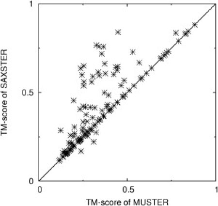
In Fig. 3 we present the TM-score data for the first template obtained by MUSTER and those obtained by SAXSTER using different profile forms and different gap-filling methods. Again, there are more targets above the diagonal line than below the diagonal line, demonstrating the improvement gained by using SAXS data compared with the original MUSTER threading alignments. However, it is worth mentioning that although SAXSTER improves the template recognition by changing the original rank of the templates, it does not attempt to modify the alignments of MUSTER. If the MUSTER program already ranks the templates with the correct shape at the top, the SAXS data cannot improve the result, which explains the unchanged templates along the diagonal lines in Fig. 3.

Figure 3.

TM-score of the first templates selected by SAXSTER versus that obtained by MUSTER. SAXS scoring functions for SAXSTER are in reciprocal space (left column) and real space (right column), respectively. Full-length models were built from a threading alignment by random walk (A and B), MODELLER (C and D), and I-TASSER (E and F).

For the successful cases, ∼93% of the templates selected by SAXSTER came from the top 10 according to the threading rank. In particular, the best templates of all of the easy cases were selected from the first 15 hits of MUSTER. Approximately 90% of the hard targets had templates picked from the first 10 threading hits, whereas the remaining targets had their best templates selected by SAXSTER from 10 up to 40 first hits according to the MUSTER rank. These data indicate that the profile-alignment-based threading algorithms have the ability to prioritize good templates in the upper part of their rank, especially for the easy targets, although they usually have difficulty in ranking the best alignments at the top, indicating that SAXSTER only needs to focus on the ranking of the top 100 MUSTER alignments (see Materials and Methods).

In Fig. 4, A–D, we show four typical examples of SAXSTER improving template recognition compared with MUSTER. Both 2FKCA and 2PJPA in Fig. 4, A and B, are multiple-domain proteins. The top MUSTER hit makes a completely incorrect alignment for 2FKCA, and has a correct alignment only for one domain for 2PJPA. The misorientation of the aligned domains resulted in the mismatched profiles with the SAXS data (see the right column of Fig. 4, A and B). The SAXS data help filter out the incorrect alignments and rank the correct template at the top. Accordingly, the TM-scores of the first templates were increased from 0.16 to 0.61 for 2FKCA, and from 0.48 to 0.81 for 2PJPA.

Figure 4.

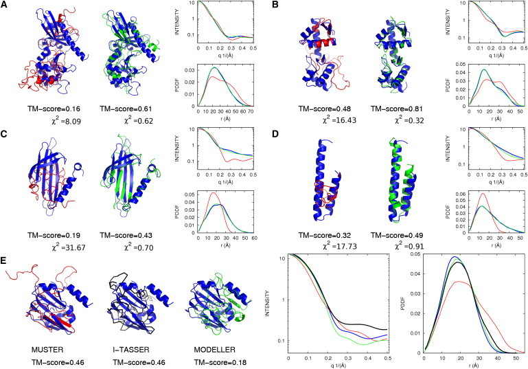
Representative examples of the protein templates selected by MUSTER and SAXSTER. Blue, red, and green cartoons represent the target structure, model from MUSTER ranking, and model from SAXSTER ranking, respectively. SAXS profiles in reciprocal and real spaces are shown for each case following the same color codes. The targets are from PDB entries (A) 2FKCA, (B) 2PJPA, (C) 2W4YA, (D) 2RKLA, and (E) 3KLRA. The black main chain in E is a SAXSTER model with loops generated by I-TASSER; all other models have loops generated by MODELLER.

2W4YA in Fig. 4 C is a single-domain protein. Although the first template of MUSTER has a shape similar to that of the target (both are globular), the SAXS profile of the template is completely different from that of the target, probably because of the different arrangement of the secondary structure that resulted in a different pairwise distance histogram. In this example, the SAXS data partly distinguish the topology of the templates despite their similar overall shape. This results in an increase in TM-score from 0.19 to 0.43.

Fig. 4 D shows a typical example of the SAXSTER improvement for single-domain proteins. The target has an elongated shape with a two-helix bundle, but the first MUSTER template has a contracted shape. The SAXS profile data rank the correct template at the top, and the TM-score increases from 0.32 to 0.49. In these four examples, the average χ²-values of the template and target SAXS profiles have decreased from 18.48 to 0.64, which demonstrates that the SAXS data were indeed the driving force behind the template improvements.

The relation of χ² in reciprocal space profiles obtained between the target and best templates from threading and SAXSTER is helpful. According to our data, if χ² between the target and the best template from SAXSTER is at least half the value of the χ² between the target and template selected by threading, a better template in fact is picked by SAXSTER. Otherwise, the balance in the scoring function between threading and SAXS terms plays a role in determining whether SAXS is useful for a particular target. Fig. 4, A–D, also show the χ²-values for threading and SAXSTER templates. In all four cases, the χ²-values for the SAXSTER models are much lower than half the value of the χ²-values for the best threading models, indicating that SAXSTER outperformed MUSTER.

Although the SAXS profiles were obtained from the target structures, it is interesting to note that there are a few cases in Fig. 3 where incorporation of the experimental SAXS data degraded the template recognition. In Fig. 4 E we show one such typical example from 3KLRA. The best template obtained by MUSTER is 1K8MA, which has both its N-terminus (1S-14T) and C-terminus (109E-125E) unaligned. The full-length structure model by MODELLER has the unaligned regions randomly stretched out (red structure in Fig. 4 E) and therefore results in distortion of the SAXS profile shape. As a result, SAXSTER picked up an incorrect template from 2JFGA, which has a better shape match (because the alignment covers the tails) but a lower TM-score (0.18 vs. 0.46). When I-TASSER was used to construct the full-length model, the tail structures of the 1K8MA template were compacted and the correct template 1K8MA was ranked as the top in SAXSTER (see black backbone in Fig. 4 E). This example highlights the importance of loop/tail modeling for SAXSTER.

Testing of SAXSTER on elongated proteins

Because the SAXS profile data essentially consist of a histogram of the pairwise distance of all atoms, it has been assumed that the SAXS score should be less sensitive to proteins of globular topology, since most globular proteins of similar sizes also have similar shapes and distance profiles. To test this assumption, we focused on proteins of elongated shape and examined the ability of SAXSTER to improve structural modeling for the SAXS-favorable cases.

Although the structures of the target proteins are usually unknown, one can use a quantitative method to categorize the protein shape from SAXS data by examining the PDDF profile. For instance, the PDDF distributions of globular particles in SAXS experiments are often symmetric in real space (Fig. 2, A′ and B′), whereas elongated particles usually have a highly asymmetric distribution (Fig. 2 D′). The critical difference between these proteins lies in the relative position of the peak value r_peak of p(r) related to the maximum intramolecular distance D_max. For a sphere particle, r_peak/D_max∼0.525, where D_max corresponds to its diameter. For proteins of elongated shape, the r_peak/D_max-value should be much smaller than 0.525. Therefore, in the new test set, we collected 141 proteins that satisfied the following criteria: 1), the SAXS PDDF peak ratio (r_peak/D_max) = <0.2, i.e., 20% of the maximum pairwise distance; and 2), the top MUSTER template has a Z-score of <7.5.

Fig. 5 shows a head-to-head comparison of the first templates obtained by MUSTER and SAXSTER. There is indeed a more significant improvement of SAXSTER on this set of elongated proteins compared with the proteins of mixed shape and topology. There are 57 proteins that have the first template with a higher TM-score than MUSTER, where in 16 cases the TM-score increase is larger than 0.25, which essentially converts nonfoldable targets into foldable targets. However, there are 78 cases in which the TM-score of SAXSTER template is unchanged. We find that in most of the latter cases, the MUSTER profile-profile alignment has already ranked the best templates at the top, and there is no room for further improvement only by template re-ranking. Overall, the average TM-score by SAXSTER increases by 18% (from 0.3394 to 0.4013). The improvement is statistically significant, corresponding to p < 10⁻⁹ in Student's t-test.

Figure 5.

TM-score of the first templates obtained by SAXSTER versus those obtained by MUSTER for 141 hard proteins with asymmetric SAXS profile distributions. The full-length models were constructed by random walk with the SAXS profile calculated in real space.

Conclusion

We have developed a new method called SAXSTER that uses SAXS data to improve template-based protein structure prediction. The strategy first extracts the SAXS profiles from C_α-based template alignments using an extended CG SAXS model. The intensity profile of each template is then matched with the SAXS data of the target proteins to prioritize the template proteins with a SAXS profile similar to that of the target. We achieved the best template recognition results when we combined the SAXS profile score with the original threading alignment scores.

We designed and tested nine different matching scoring functions to compare the template profile and the SAXS data for the target. Although all scores showed some degree of recognition ability for template structures, the logarithm of integrated correlation score (Scheme IX in Table S1) showed the best template prioritizing ability and had the highest correlation with the true TM-score of the target structures.

We tested SAXSTER on 412 nonredundant proteins. We found that the SAXS profile data could consistently improve the overall result of the template recognition of current threading alignments. Because threading alignments usually have gaps, we exploited three methods (random walk, MODELLER, and I-TASSER) to quickly construct the structure of the missed structural region. Although the template recognition results are somewhat sensitive to loop/tail reconstruction accuracy from threading alignment, all of the improvements over the original threading program were statistically significant, with p-values ranging from 10⁻⁶ to 10⁻⁸.

To examine the SAXS performance on proteins of elongated shape, we collected a second set of 141 hard proteins with asymmetric SAXS profile distributions. The average TM-score of the first templates was improved by SAXSTER by 18%, which corresponds to p < 10⁻⁹ in Student's t-test. In 16 cases, the template TM-score increased by >0.25, which essentially converted the nonfoldable protein targets into foldable ones.

Although we obtained encouraging results by using the SAXS data, it should be noted that in this work we focused only on re-ranking and selecting the threading templates without modifying the threading alignments. If the threading algorithms fail to correctly align the target with the template, or the PDB library lacks appropriate templates, SAXSTER is unable to obtain correct structural models. A more intensive use of the SAXS data would be to exploit the SAXS profile as shape constraints to guide the structural assembly simulation in an approach such as I-TASSER (16,31). Because the SAXS profile score is most sensitive to proteins of irregular shape, we expect that a more promising use of the SAXSTER algorithm would be to improve the template recognition results for multiple-domain proteins or protein-protein complexes (32). Work in that direction is currently in progress.

References

- 1.Kopp J., Bordoli L., Schwede T. Assessment of CASP7 predictions for template-based modeling targets. Proteins. 2007;69(Suppl 8):38–56. doi: 10.1002/prot.21753. [DOI] [PubMed] [Google Scholar]
- 2.Cozzetto D., Kryshtafovych A., Tramontano A. Evaluation of template-based models in CASP8 with standard measures. Proteins. 2009;77(Suppl 9):18–28. doi: 10.1002/prot.22561. [DOI] [PMC free article] [PubMed] [Google Scholar]
- 3.Berman H.M., Westbrook J., Bourne P.E. The Protein Data Bank. Nucleic Acids Res. 2000;28:235–242. doi: 10.1093/nar/28.1.235. [DOI] [PMC free article] [PubMed] [Google Scholar]
- 4.Bowie J.U., Lüthy R., Eisenberg D. A method to identify protein sequences that fold into a known three-dimensional structure. Science. 1991;253:164–170. doi: 10.1126/science.1853201. [DOI] [PubMed] [Google Scholar]
- 5.Jones D.T., Taylor W.R., Thornton J.M. A new approach to protein fold recognition. Nature. 1992;358:86–89. doi: 10.1038/358086a0. [DOI] [PubMed] [Google Scholar]
- 6.DiMaio F., Terwilliger T.C., Baker D. Improved molecular replacement by density- and energy-guided protein structure optimization. Nature. 2011;473:540–543. doi: 10.1038/nature09964. [DOI] [PMC free article] [PubMed] [Google Scholar]
- 7.Raman S., Lange O.F., Baker D. NMR structure determination for larger proteins using backbone-only data. Science. 2010;327:1014–1018. doi: 10.1126/science.1183649. [DOI] [PMC free article] [PubMed] [Google Scholar]
- 8.Li W., Zhang Y., Skolnick J. Application of sparse NMR restraints to large-scale protein structure prediction. Biophys. J. 2004;87:1241–1248. doi: 10.1529/biophysj.104.044750. [DOI] [PMC free article] [PubMed] [Google Scholar]
- 9.Xu Y., Xu D., Einstein J.R. A computational method for NMR-constrained protein threading. J. Comput. Biol. 2000;7:449–467. doi: 10.1089/106652700750050880. [DOI] [PubMed] [Google Scholar]
- 10.Putnam C.D., Hammel M., Tainer J.A. X-ray solution scattering (SAXS) combined with crystallography and computation: defining accurate macromolecular structures, conformations and assemblies in solution. Q. Rev. Biophys. 2007;40:191–285. doi: 10.1017/S0033583507004635. [DOI] [PubMed] [Google Scholar]
- 11.Zheng W., Doniach S. Fold recognition aided by constraints from small angle X-ray scattering data. Protein Eng. Des. Sel. 2005;18:209–219. doi: 10.1093/protein/gzi026. [DOI] [PubMed] [Google Scholar]
- 12.Wu S., Zhang Y. MUSTER: improving protein sequence profile-profile alignments by using multiple sources of structure information. Proteins. 2008;72:547–556. doi: 10.1002/prot.21945. [DOI] [PMC free article] [PubMed] [Google Scholar]
- 13.Wang G., Dunbrack R.L., Jr. PISCES: a protein sequence culling server. Bioinformatics. 2003;19:1589–1591. doi: 10.1093/bioinformatics/btg224. [DOI] [PubMed] [Google Scholar]
- 14.Sali A., Blundell T.L. Comparative protein modelling by satisfaction of spatial restraints. J. Mol. Biol. 1993;234:779–815. doi: 10.1006/jmbi.1993.1626. [DOI] [PubMed] [Google Scholar]
- 15.Zhang Y. Template-based modeling and free modeling by I-TASSER in CASP7. Proteins. 2007;69(Suppl 8):108–117. doi: 10.1002/prot.21702. [DOI] [PubMed] [Google Scholar]
- 16.Roy A., Kucukural A., Zhang Y. I-TASSER: a unified platform for automated protein structure and function prediction. Nat. Protoc. 2010;5:725–738. doi: 10.1038/nprot.2010.5. [DOI] [PMC free article] [PubMed] [Google Scholar]
- 17.Fraser R.D.B., Macrae T.P., Suzuki E. An improved method for calculating the contribution of solvent to x-ray diffraction pattern of biological molecules. J. Appl. Cryst. 1978;11:693–694. [Google Scholar]
- 18.Wilson A.J.C., editor. International Tables for Crystallography. Kluwer Academic Publishers; Dordrecht/Boston/London: 1992. [Google Scholar]
- 19.Svergun D., Barberato C., Koch M.H.J. CRYSOL—a program to evaluate x-ray solution scattering of biological macromolecules from atomic coordinates. J. Appl. Cryst. 1995;28:768–773. [Google Scholar]
- 20.Svergun D.I., Richard S., Zaccai G. Protein hydration in solution: experimental observation by x-ray and neutron scattering. Proc. Natl. Acad. Sci. USA. 1998;95:2267–2272. doi: 10.1073/pnas.95.5.2267. [DOI] [PMC free article] [PubMed] [Google Scholar]
- 21.Petoukhov M.V., Svergun D.I. New methods for domain structure determination of proteins from solution scattering data. J. Appl. Cryst. 2003;36:540–544. [Google Scholar]
- 22.Förster F., Webb B., Sali A. Integration of small-angle X-ray scattering data into structural modeling of proteins and their assemblies. J. Mol. Biol. 2008;382:1089–1106. doi: 10.1016/j.jmb.2008.07.074. [DOI] [PMC free article] [PubMed] [Google Scholar]
- 23.Glatter O., Kratky O., editors. Small Angle X-Ray Scattering. Academic Press; London: 1982. [Google Scholar]
- 24.Yang S., Park S., Roux B. A rapid coarse residue-based computational method for x-ray solution scattering characterization of protein folds and multiple conformational states of large protein complexes. Biophys. J. 2009;96:4449–4463. doi: 10.1016/j.bpj.2009.03.036. [DOI] [PMC free article] [PubMed] [Google Scholar]
- 25.Franke D., Svergun D.I. DAMMIF, a program for rapid ab-initio shape determination in small-angle scattering. J. Appl. Cryst. 2009;42:342–346. doi: 10.1107/S0021889809000338. [DOI] [PMC free article] [PubMed] [Google Scholar]
- 26.Kozin M.B., Svergun D.I. Automated matching of high- and low-resolution structural models. J. Appl. Cryst. 2001;34:33–41. [Google Scholar]
- 27.Winn M.D., Ashton A.W., Patel P. Ongoing developments in CCP4 for high-throughput structure determination. Acta Crystallogr. D Biol. Crystallogr. 2002;58:1929–1936. doi: 10.1107/s0907444902016116. [DOI] [PubMed] [Google Scholar]
- 28.Schneidman-Duhovny D., Hammel M., Sali A. FoXS: a web server for rapid computation and fitting of SAXS profiles. Nucleic Acids Res. 2010;38(Web Server issue) doi: 10.1093/nar/gkq461. W540–4. [DOI] [PMC free article] [PubMed] [Google Scholar]
- 29.Svergun D.I. Determination of the regularization parameter in indirect-transform methods using perceptual criteria. J. Appl. Cryst. 1992;25:495–503. [Google Scholar]
- 30.Hura G.L., Menon A.L., Tainer J.A. Robust, high-throughput solution structural analyses by small angle X-ray scattering (SAXS) Nat. Methods. 2009;6:606–612. doi: 10.1038/nmeth.1353. [DOI] [PMC free article] [PubMed] [Google Scholar]
- 31.Zhang Y. I-TASSER: fully automated protein structure prediction in CASP8. Proteins. 2009;77(Suppl 9):100–113. doi: 10.1002/prot.22588. [DOI] [PMC free article] [PubMed] [Google Scholar]
- 32.Mukherjee S., Zhang Y. Protein-protein complex structure predictions by multimeric threading and template recombination. Structure. 2011;19:955–966. doi: 10.1016/j.str.2011.04.006. [DOI] [PMC free article] [PubMed] [Google Scholar]
Associated Data
This section collects any data citations, data availability statements, or supplementary materials included in this article.