On the covariate-adjusted estimation for an overall treatment difference with data from a randomized comparative clinical trial

Abstract

To estimate an overall treatment difference with data from a randomized comparative clinical study, baseline covariates are often utilized to increase the estimation precision. Using the standard analysis of covariance technique for making inferences about such an average treatment difference may not be appropriate, especially when the fitted model is nonlinear. On the other hand, the novel augmentation procedure recently studied, for example, by Zhang and others (2008. Improving efficiency of inferences in randomized clinical trials using auxiliary covariates. Biometrics 64, 707–715) is quite flexible. However, in general, it is not clear how to select covariates for augmentation effectively. An overly adjusted estimator may inflate the variance and in some cases be biased. Furthermore, the results from the standard inference procedure by ignoring the sampling variation from the variable selection process may not be valid. In this paper, we first propose an estimation procedure, which augments the simple treatment contrast estimator directly with covariates. The new proposal is asymptotically equivalent to the aforementioned augmentation method. To select covariates, we utilize the standard lasso procedure. Furthermore, to make valid inference from the resulting lasso-type estimator, a cross validation method is used. The validity of the new proposal is justified theoretically and empirically. We illustrate the procedure extensively with a well-known primary biliary cirrhosis clinical trial data set.

1. INTRODUCTION

For a typical randomized clinical trial to compare two treatments, generally a summary measure θ₀ for quantifying the treatment effectiveness difference can be estimated unbiasedly or consistently using its simple two-sample empirical counterpart, say $\widehat{\theta }$. With the subject's baseline covariates, one may obtain a more efficient estimator for θ₀ via a standard analysis of covariance (ANCOVA) technique or a novel augmentation procedure, which is well documented in Zhang and others (2008) and a series of papers (Leon and others, 2003, Tsiatis, 2006, Tsiatis and others, 2008, Lu and Tsiatis, 2008, Gilbert and others, 2009, Zhang and Gilbert, 2010). The ANCOVA approach can be problematic, especially when the regression model is nonlinear, for example, the logistic or Cox model. For this case, the ANCOVA estimator generally does not converge to θ₀, but to a quantity which may be difficult to interpret as a treatment contrast measure. Moreover, in the presence of censored event time observations, this quantity may depend on the censoring distribution. On the other hand, the above augmentation procedure, referred as ZTD, in the literature always produces a consistent estimator for θ₀, provided that the simple estimator $\widehat{\theta }$ is consistent.

In theory, the ZTD estimator, denoted by ${\widehat{\theta }}_{\text{ZTD}}$ hereafter, is asymptotically more efficient than $\widehat{\theta }$ no matter how many covariates being augmented. In practice, however, an “overly augmented” or “mis-augmented” estimator may have a larger variance than that of $\widehat{\theta }$ and in special case may even have undesirable finite sample bias. Recently, Zhang and others (2008) showed empirically that the ZTD via the standard stepwise regression for variable selection performs satisfactorily when the number of covariates is not large. In general, however, it is not clear that the standard inference procedures for θ₀ based on estimators augmented by covariates selected via a rather complex variable selection process is appropriate especially when the number of covariates involved is not small relative to the sample size. Therefore, it is highly desirable to develop an estimation procedure to properly and systematically augment $\widehat{\theta }$ and make valid inference for the treatment difference using the data with practical sample sizes.

Now, let Y be the response variable, T be the binary treatment indicator, and Z be a p-dimensional vector of baseline covariates including 1 as its first element and possibly transformations of original variables. The data, {(Y_i,T_i,Z_i),i = 1,…,n}, consist of n independent copies of (Y,T,Z), where T and Z are independent of each other. Let P(T = 1) = π∈(0,1). First, suppose that we are interested in the mean difference: θ₀ = E(Y|T = 1) − E(Y|T = 0). A simple unadjusted estimator is

which consistently estimates θ₀. To improve efficiency in estimating θ₀, one may employ the standard ANCOVA procedure by fitting the following linear regression “working” model:

where θ and γ are unknown parameters. Since T⊥Z and {(T_i,Z_i),i = 1,…,n} are independent copies of (T,Z), the resulting ANCOVA estimator is asymptotically equivalent to

(1.1)

where $\widehat{\gamma }$ is the ordinary least square estimator for γ of the model E(Y|Z) = γ^′Z. As n→∞,$\widehat{\gamma }$ converges to

It follows that the ANCOVA estimator is asymptotically equivalent to

(1.2)

In theory, since $\widehat{\theta }$ is consistent to θ₀, the ANCOVA estimator is also consistent to θ₀ and more efficient than $\widehat{\theta }$ regardless of whether the above working model is correctly specified. Furthermore, as noted by Tsiatis and others (2008), the nonparametric ANCOVA estimator proposed by Koch and others (1998) and ${\widehat{\theta }}_{\text{ZTD}}$ are also asymptotically equivalent to (1.2) when π = 0.5. We give details of this equivalence in Appendix A.

The novel ZTD procedure is derived by specifying optimal estimating functions under a very general semi-parametric setting. The efficiency gain from ${\widehat{\theta }}_{\text{ZTD}}$ has been elegantly justified using the semi-parametric inference theory (Tsiatis, 2006). The ZTD is much more flexible than the ANCOVA method in that it can handle cases when the summary measure θ₀ is beyond the simple difference of two group means. On the other hand, the ANCOVA method may only work under above simple linear regression model.

In this paper, we study the estimator (1.1), which augments $\widehat{\theta }$ directly with the covariates. The key question is how to choose $\widehat{\gamma }$ in (1.1) especially when p is not small with respect to n. Here, we utilize the lasso procedure with a cross validation process to construct a systematic procedure for selecting covariates to increase the estimation precision. The validity of the new proposal is justified theoretically and empirically via an extensive simulation study. The proposal is also illustrated with the data from a clinical trial to evaluate a treatment for a specific liver disease.

2. ESTIMATING THE TREATMENT DIFFERENCE VIA PROPER AUGMENTATION FROM COVARIATES

For a general treatment contrast measure θ₀ and its simple two-sample estimator $\widehat{\theta }$, assume that

where τ_i(η) is the influence function from the ith observation, η is a vector of unknown parameters, and i = 1,…,n. Note that the influence function generally only involves a rather small number of unknown parameters, which is not dependent on Z. Let $\widehat{\eta }$ denote the consistent estimator for η. Generally, the above asymptotic expansion is also valid with τ_i being replaced by ${\tau }_i(\widehat{\eta })$. Now, (1.2) can be rewritten as

where ξ_i = (T_i − π)Z_i/{π(1 − π)},i = 1,…,n. Then $\widehat{\gamma }$ in (1.1) is the minimizer of

(2.1)

When the dimension of Z is not small, to obtain a stable minimizer, one may consider the following regularized minimand:

where λ is the lasso tuning parameter (Tibshirani, 1996) and |·| denote the L₁ norm for a vector. For any fixed λ, let the resulting minimizer be denoted by $\widehat{\gamma }\left(\lambda \right).$ The corresponding augmented estimator and its variance estimator are

and

(2.2)

respectively. Asymptotically, one may ignore the variability of $\widehat{\gamma }\left(\lambda \right)$ and treat it as a constant when we make inferences about θ₀. However, in some cases, we have found empirically that similar to ${\widehat{\theta }}_{\text{ZTD}}$, ${\widehat{\theta }}_{\text{lasso}}\left(\lambda \right)$ is biased partly due to the fact that $\widehat{\gamma }\left(\lambda \right)$ and {ξ_i,i = 1,…,n} are correlated. In the simulation study, we show via a simple example this undesirable finite-sample phenomenon. In practice, such bias may not have real impact on the conclusions about the treatment difference, θ₀, when the study sample size is relatively large with respect to the dimension of Z.

One possible solution to reduce the correlation between $\widehat{\gamma }\left(\lambda \right)$ and ξ_i is to use a cross validation procedure. Specifically, we randomly split the data into K nonoverlapping sets {𝒟₁,…,𝒟_K} and construct an estimator for θ₀:

where i∈𝒟_ki, ${\widehat{\gamma }}_{(-i)}\left(\lambda \right)$ is the minimizer of

and ${\widehat{\eta }}_{(-i)}$ is a consistent estimator for η with all data but not from 𝒟_ki. Note that ${\widehat{\gamma }}_{(-i)}\left(\lambda \right)$ and ξ_i are independent and no extra bias would be added from ${\widehat{\theta }}_{\text{cv}}\left(\lambda \right)$ to $\widehat{\theta }.$ When n>p, the variance of ${\widehat{\theta }}_{\text{cv}}\left(\lambda \right)$ can be estimated by ${\widehat{V}}_{\text{lasso}}\left(\lambda \right)$ given in (2.4). However ${\widehat{V}}_{\text{lasso}}\left(\lambda \right)$ tends to underestimate its true variance when p is not small.

Here, we utilize the above cross validation procedure to construct a natural variance estimator:

In Appendix B, we justify that this estimator is better than ${\widehat{V}}_{\text{lasso}}\left(\lambda \right)$. Moreover, when λ is close to zero and p is large, that is, one almost uses the standard least square procedure to obtain ${\widehat{\gamma }}_{(-i)}\left(\lambda \right),$ the above variance estimate can be modified slightly for improving its estimation accuracy (see Appendix B for details). A natural “optimal” estimator using the above lasso procedure is ${\widehat{\theta }}_{\text{opt}}={\widehat{\theta }}_{\text{cv}}(\widehat{\lambda }),$ where $\widehat{\lambda }$ is the penalty parameter value, which minimizes ${\widehat{V}}_{\text{cv}}\left(\lambda \right)$ over a range of λ values of interest. As a referee kindly pointed out, when θ₀ is the mean difference, one may replace (2.3) by the simple least squared objective function

without the need of estimating the influence function.

3. APPLICATIONS

In this section, we show how to apply the new estimation procedure to various cases. To this end, we only need to determine the initial estimate $\widehat{\theta }$ for the contrast measure of interest and its corresponding first-order expansion in each application. First, we consider the case that the response is continuous or binary and the group mean difference is the parameter of interest. Here,

In this case, it is straightforward to show that

where η = (μ₁,μ₀)^′, ${\widehat{\mu }}_1=\sum _{i=1}^n{T}_i{Y}_i/\pi n,$ and ${\widehat{\mu }}_0=\sum _{i=1}^n(1-T_i)Y_i/(1-\pi )n.$

Now, when the response is binary with success rate p_j for the treatment group j,j = 0,1, but θ₀ = log{p₁(1 − p₀)/p₀/(1 − p₁)}, then

where ${\widehat{p}}_1=\sum _{i=1}^n{T}_i{Y}_i/\pi n,$ and ${\widehat{p}}_0=\sum _{i=1}^n(1-T_i)Y_i/(1-\pi )n.$ For this case,

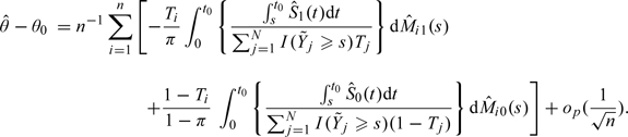
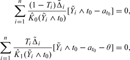
Last, we consider the case when Y is the time to a specific event but may be censored by an independent censoring variable. To be specific, we observe $(\stackrel{\sim }{Y},\Delta )$ where $\stackrel{\sim }{Y}=YandC,$Δ = I(Y < C), C is the censoring time, and I(·) is the indicator function. A most commonly used summary measure for quantifying the treatment difference in survival analysis is the ratio of two hazard functions. The two sample Cox estimator is often used to estimate such a ratio. However, when the proportional hazards assumption between two groups is not valid, this estimator converges to a parameter which may be difficult to interpret as a measure of the treatment difference. Moreover, this parameter depends on the censoring distribution. Therefore, it is desirable to use a model-free summary measure for the treatment contrast. One may simply use the survival probability at a given time t₀ as a model-free summary for survivorship. For this case, θ₀ = P(Y > t₀|T = 1) − P(Y > t₀|T = 0) and $\widehat{\theta }={\widehat{S}}_1(t_0)-{\widehat{S}}_0(t_0),$ where ${\widehat{S}}_j(·)$ is the Kaplan–Meier estimator of the survival function of Y in group j,j = 0,1. For this case,

where

and ${\widehat{\lambda }}_j(·)$ is the Nelson–Alan estimator for the cumulative hazard function of Y in group j (Flemming and Harrington, 1991).

To summarize a global survivorship beyond using t-year survival rates, one may use the mean survival time. Unfortunately, in the presence of censoring, such a measure cannot be estimated well. An alternative is to use the so-called restricted mean survival time, that is, the area under the survival function up to time point t₀. The corresponding consistent estimator is the area under the Kaplan–Meier curve. For this case, θ₀ = E(Yandt₀|T = 1) − E(Yandt₀|T = 0) and

For this case,

4. A SIMULATION STUDY

We conducted an extensive simulation study to examine the finite sample performance of the new estimates ${\widehat{\theta }}_{\text{cv}}\left(\lambda \right)$ and ${\widehat{\theta }}_{\text{opt}}$ for θ₀. First, we investigate whether ${\widehat{V}}_{\text{cv}}\left(\lambda \right)$ estimates the true variance of ${\widehat{\theta }}_{\text{cv}}\left(\lambda \right)$ well under various practical settings. We also examine the finite sample properties for the interval estimation procedure based on the optimal ${\widehat{\theta }}_{\text{opt}}.$ To this end, we consider the following models for generating the underlying data:

1. the linear regression model with continuous response

   
2. the logistic regression model with binary response

   
3. the Cox regression model with survival response

   

where ε₀ and censoring time are generated from the unit exponential distribution and U(0,3), respectively, and we are interested in survival curves over the time interval [0,t₀] = [0,2.5].

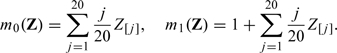
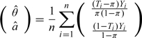
Throughout we let n = 200 and generate (Z_[1],…,Z_[100])^′ from multivariate normal distribution with mean 0, variance 1, and a compound symmetry covariance ℘ chosen to be either 0 or 0.5. For each generated data set, the 20-fold cross validation is used to calculate ${\widehat{\theta }}_{\text{cv}}\left(\lambda \right)$ and ${\widehat{V}}_{\text{cv}}\left(\lambda \right)$ over a sequence of tuning parameters {λ₁,λ₂,…,λ₁₀₀}, where λ₁ is chosen such that $\widehat{\gamma }({\lambda }_1)=0$ for all simulated data sets, λ_k = 10 ^{− 3/98}λ_{k − 1} for k = 2,…,99 and λ₁₀₀ = 0. In the first set of simulation, we set

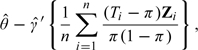
All the results are summarized based on 5000 replications. In Figure 1, we present the average of ${\widehat{V}}_{\text{cv}}\left(\lambda \right)$, the average of ${\widehat{V}}_{\text{lasso}}\left(\lambda \right)$, and the empirical variance of ${\widehat{\theta }}_{\text{cv}}\left(\lambda \right)$ when ℘ = 0 for continuous, binary, and survival responses, respectively. The results suggest that ${\widehat{V}}_{\text{cv}}\left(\lambda \right)$ approximates the true variance of ${\widehat{\theta }}_{\text{cv}}\left(\lambda \right)$ very well; while ${\widehat{V}}_{\text{lasso}}\left(\lambda \right)$ obtained without cross validation tends to severely underestimate the true variance. When the covariates are correlated with ℘ = 0.5, the corresponding results are presented in Figure 1. The results are consistent with the case with ℘ = 0.

Fig. 1.

Comparing various estimates for ${\widehat{\theta }}_{\text{cv}}\left(\lambda \right)$ at {λ₁,…,λ₁₀₀}: the empirical variance of ${\widehat{\theta }}_{\text{cv}}\left(\lambda \right)$ (black curve); ${\widehat{V}}_{\text{cv}}\left(\lambda \right)$ (dashed curve); ${\widehat{V}}_{\text{lasso}}\left(\lambda \right)$ (grey curve); (a–c) for independent coviariate; (d–f) for dependent covariate.

Next, we examine the performance of the optimal estimator ${\widehat{\theta }}_{\text{opt}}={\widehat{\theta }}_{cv}(\widehat{\lambda })$, where $\widehat{\lambda }$ is chosen to be the minimizer of ${\widehat{V}}_{\text{cv}}\left(\lambda \right),\lambda \in \{{\lambda }_1,\dots ,{\lambda }_{100}\}.$ For each simulated data set, we construct a 95% confidence intervals (CI) based on ${\widehat{\theta }}_{\text{opt}}$ and ${\widehat{V}}_{\text{opt}}={\widehat{V}}_{\text{cv}}(\widehat{\lambda }).$ We summarized results from the 5000 replications based on the empirical bias, standard error, and coverage level and length of the constructed CIs. For comparisons, we also obtain those values based on the simple estimator $\widehat{\theta },$${\widehat{\theta }}_{\text{ZTD}}$, and ${\widehat{\theta }}_{\text{cv}}({\lambda }_0)$ along with their variance estimators, where λ₀ is the minimizer of the empirical variance of ${\widehat{\theta }}_{\text{cv}}({\lambda }_0)$. In all the numerical studies, the forward subset selection procedure coupled with BIC is used to select variables for the efficiency augmentation in the ZTD procedure. The results are summarized in Table 1. The coverage levels for ${\widehat{\theta }}_{\text{opt}}$ are close to the nominal counterparts and the interval lengths are almost identical to those based on the estimate with the true optimal λ₀. On the other hand, the simple estimate $\widehat{\theta }$ tends to have substantially wider interval estimates than ${\widehat{\theta }}_{\text{opt}}$, ${\widehat{\theta }}_{\text{cv}}({\lambda }_0)$, and ${\widehat{\theta }}_{\text{ZTD}}$. The empirical standard error of ${\widehat{\theta }}_{\text{ZTD}}$ is slightly greater than that of ${\widehat{\theta }}_{\text{opt}}$ or ${\widehat{\theta }}_{\text{cv}}({\lambda }_0),$ which implies the advantages of lasso procedure. More importantly, the naive variance estimator of ${\widehat{\theta }}_{\text{ZTD}}$ may severely underestimate the true variance and thus results in much more liberal confidence interval estimation procedure, which potentially can be corrected via cross validation. In summary, for all cases studied, the augmented estimators can substantially improve the efficiency of $\widehat{\theta }$ in terms of narrowing the average length of the confidence interval of θ₀ and ${\widehat{\theta }}_{\text{opt}}$-based inference is more reliable than that based on ${\widehat{\theta }}_{\text{ZTD}}$. Furthermore, in the variance estimation for ${\widehat{\theta }}_{\text{opt}}={\widehat{\theta }}_{\text{cv}}(\widehat{\lambda }),$ the variability in $\widehat{\lambda }$ may cause slightly downward bias, which is almost negligible in our empirical studies. Last, all estimators considered here are almost unbiased in the first set of simulation.

Table 1.

The empirical bias, standard error, and coverage levels and lengths for the 0.95 CI based on $\widehat{\theta }$, ${\widehat{\theta }}_{\text{opt}}$, ${\widehat{\theta }}_{\text{cv}}\left({\lambda }_0\right)$, and ${\widehat{\theta }}_{\text{ZTD}}$

Response	Estimator	Independent covariates				Correlated covariates
		BIAS	ESE	EAL (10−3)	ECL (%)	BIAS	ESE	EAL (10−3)	ECL (%)
Continuous	$\widehat{\theta }$	0.007	0.403	1.580 (1.1†)	94.9	– 0.005	1.100	4.264 (3.0)	94.4
	${\widehat{\theta }}_{\text{opt}}$	0.002	0.169	0.648 (0.6)	94.2	0.001	0.166	0.743 (1.9)	97.0
	${\widehat{\theta }}_{\text{cv}}\left({\lambda }_0\right)$	0.002	0.167	0.652 (0.6)	94.7	0.001	0.163	0.749 (1.9)	97.3
	${\widehat{\theta }}_{\text{ZTD}}$	0.003	0.204	0.622 (0.6)	87.2	– 0.001	0.359	0.749 (1.8)	72.6
Binary	$\widehat{\theta }$	0.009	0.291	1.136 (0.2)	95.1	0.004	0.271	1.047 (0.3)	94.6
	${\widehat{\theta }}_{\text{opt}}$	0.003	0.245	0.946 (0.7)	94.6	0.004	0.191	0.745 (0.5)	95.2
	${\widehat{\theta }}_{\text{cv}}\left({\lambda }_0\right)$	0.003	0.243	0.953 (0.7)	94.9	0.003	0.189	0.747 (0.5)	95.5
	${\widehat{\theta }}_{\text{ZTD}}$	– 0.011	0.259	0.822 (0.7)	88.9	– 0.005	0.201	0.508 (0.7)	78.9
Survival	$\widehat{\theta }$	0.003	0.164	0.626 (0.2)	94.1	0.005	0.173	0.665 (0.1)	94.5
	${\widehat{\theta }}_{\text{opt}}$	0.001	0.127	0.476 (0.4)	93.7	0.005	0.112	0.426 (0.3)	93.9
	${\widehat{\theta }}_{\text{cv}}\left({\lambda }_0\right)$	0.001	0.127	0.479 (0.4)	94.0	0.005	0.111	0.427 (0.3)	94.2
	${\widehat{\theta }}_{\text{ZTD}}$	0.004	0.141	0.457 (0.4)	89.5	0.005	0.122	0.401 (0.3)	89.8
Continuous	$\widehat{\theta }$	0.019	0.876	3.476 (2.6)	94.9	0.009	1.502	5.499 (4.4)	93.0
	${\widehat{\theta }}_{\text{opt}}$	0.002	0.533	2.084 (2.0)	94.4	– 0.038	1.188	4.618 (8.4)	93.9
	${\widehat{\theta }}_{\text{cv}}\left({\lambda }_0\right)$	0.016	0.530	2.097 (2.0)	94.8	0.069	1.191	4.685 (8.7)	94.5
	${\widehat{\theta }}_{\text{ZTD}}$	– 0.159	0.583	2.068 (2.2)	91.1	0.390	1.305	4.193 (7.1)	88.9
Binary	$\widehat{\theta }$	0.023	0.288	1.130 (0.2)	94.3	– 0.001	0.290	1.140 (0.3)	95.4
	${\widehat{\theta }}_{\text{opt}}$	0.017	0.242	0.935 (0.7)	94.7	– 0.003	0.188	0.753 (0.6)	95.4
	${\widehat{\theta }}_{\text{cv}}\left({\lambda }_0\right)$	0.021	0.240	0.941 (0.7)	95.0%	0.002	0.187	0.757 (0.6)	95.7
	${\widehat{\theta }}_{\text{ZTD}}$	– 0.023	0.265	0.855 (0.8)	88.8	– 0.006	0.201	0.546 (0.7)	82.8
Survival	$\widehat{\theta }$	– 0.003	0.173	0.659 (0.1)	93.7	0.010	0.173	0.663 (0.1)	94.6
	${\widehat{\theta }}_{\text{opt}}$	– 0.005	0.141	0.531 (0.4)	93.6	0.005	0.114	0.431 (0.3)	94.4
	${\widehat{\theta }}_{\text{cv}}\left({\lambda }_0\right)$	– 0.002	0.140	0.534 (0.4)	93.8	0.007	0.114	0.433 (0.3)	94.6
	${\widehat{\theta }}_{\text{ZTD}}$	– 0.023	0.157	0.515 (0.4)	89.4	0.014	0.120	0.411 (0.3)	91.4

BIAS, empirical bias; ESE, empirical standard error of the estimator; EAL, empirical average length; and ECL: empirical coverage level.

^†The Monte Carlo standard error in estimating the average length.

For the second set of simulation, we repeat the above numerical study with

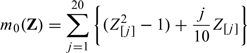and

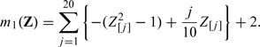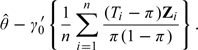
We augment the simple estimator by Z = (Z_[1],…,Z_[40],Z_[1]²,…,Z_[40]²)^′. The corresponding results are reported in Figure 2(a–f) and Table 1. The results are similar to those from the first set of simulation study except that for the continuous outcome, the empirical bias of ${\widehat{\theta }}_{\text{ZTD}}$ is not trivial relative to the corresponding standard error. On the other hand, the estimate ${\widehat{\theta }}_{\text{opt}}$ is almost unbiased for all cases as ensured by the cross validation procedure. Note that without knowing the practical meanings of the response, the absolute magnitude of the bias alone is difficult to interpret and a seemingly substantial bias relative to the standard error may still be irrelevant in practice. However, the presence of such a bias still poses a risk in making statistical inference on marginal treatment effect. In further simulations (not reported), we have found that the bias cannot be completely eliminated by increasing sample size or including quadratic transformation in Z. Last, we would like to pointed out the presence of bias is a uncommon finite sample phenomenon and does not undermine the asymptotical validity of ZTD and similar procedures. For example, under the aforementioned setup if we reduce the dimension of Z to 10 and increase the sample size to 500, then the bias becomes essentially 0.

Fig. 2.

Comparing various estimates for ${\widehat{\theta }}_{\text{cv}}\left(\lambda \right)$ at {λ₁,…,λ₁₀₀}: the empirical variance of ${\widehat{\theta }}_{\text{cv}}\left(\lambda \right)$ (black curve); ${\widehat{V}}_{\text{cv}}\left(\lambda \right)$ (dashed curve); ${\widehat{V}}_{\text{lasso}}\left(\lambda \right)$ (grey curve) ; (a–c) for independent coviariate; (d–f) for dependent covariate.

For the third set of simulation, we examine the potential efficiency loss due to not including important nonlinear transformations of baseline covariates in the efficiency augmentation. To this end, we simulate continuous, binary and survival outcomes as in the previous stimulation study with

and

We augment the efficiency of the initial estimator first by Z₁ = (Z_[1],…,Z_[100])^′ and second by Z₂ = (Z_[1],…,Z_[100],Z_[1]²,…,Z_[20]²)^′. In Table 2, we present the empirical bias and standard error of ${\widehat{\theta }}_{\text{opt}}$ based on 5000 replications. As expected, the empirical performance of the estimator augmented by Z₂ is superior to that of its counterpart using Z₁. The gains in efficiency for binary and survival outcomes are less significant than that for continuous outcome, which is likely due to the fact that the influence function of $\widehat{\theta }$ is neither a linear nor a quadratic function of Z_[j],j = 1,…,100 in the binary or survival setting.

Table 2.

The empirical bias and standard error of ${\widehat{\theta }}_{\text{opt}}$ augmented by Z₁ and Z₂

Response	Augmentation vector	Independent covariates		Correlated covariates
		BIAS	ESE	BIAS	ESE
Continuous	Z1	– 0.024	0.770	– 0.085	1.831
	Z2	– 0.020	0.745	– 0.035	1.492
Binary	Z1	– 0.001	0.261	– 0.004	0.239
	Z2	0.001	0.258	– 0.002	0.226
Survival	Z1	0.037	0.156	0.004	0.133
	Z2	0.037	0.154	0.003	0.124

BIAS, empirical bias; ESE, empirical standard error.

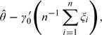
In the fourth set of simulation, we examine the “null model” setting in which none of the covariates are related to the response. To this end, we generate continuous responses Y from the normal distribution N(0,1) for T = 0 and N(1,1) for T = 1. The covariate Z is from a standard multivariate normal distribution generated independent of Y. For each generated data set, we obtain the optimal estimator ${\widehat{\theta }}_{\text{opt}}$ and its variance estimator as in the previous simulation study. Based on 3000 replications, we estimate the empirical variance of ${\widehat{\theta }}_{\text{opt}}$ and the average of the variance estimator for given combination of n and p. To examine the effect of “overadjustment”, we let p = 0,20,40,…,780 and 800 while fixing the sample size n at 200. In Figure 3, we present the empirical average for ${\widehat{V}}_{\text{cv}}(\widehat{\lambda })$ (dashed curve) and the empirical variance of ${\widehat{\theta }}_{\text{opt}}$ (solid curve). The optimal estimator is the naive estimator $\widehat{\theta }$ without any covariate-based augmentation in this case. The figure demonstrates that the variance of ${\widehat{\theta }}_{\text{opt}}$ increases very slowly with the dimension p and is still near the optimal level even with 800 noise covariates. The variance estimator slightly underestimates the true variance and the downward bias increases with the dimension p, which could be attributable to the fact that we use ${\widehat{V}}_{cv}(\widehat{\lambda })={min}_{\lambda }\{{\widehat{V}}_{\text{cv}}\left(\lambda \right)\}$ as the variance estimator without any adjustments. On the other hand, the bias remains rather low ( < 6% of the empirical variance) such that the valid inference on θ₀ can still be made over the entire range of p. In Figure 3, we represent the similar results with noise covariates generated from dependent multivariate normal distribution as in the previous simulation studies.

Fig. 3.

Empirical variance of ${\widehat{\theta }}_{\text{opt}}$ (wiggly solid curve) and its variance estimator (dashed curve) in the presence of high-dimensional noise covariates. The horizontal solid curve presents the optimal variance level.

5. AN EXAMPLE

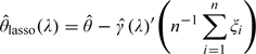
We illustrate the new proposal with the data from a clinical trial to compare d-penicillmain and placebo for patients with primary biliary cirrhosis (PBC) of liver (Therneau and Grambsch, 2000). The primary endpoint is the time to death. The trial was conducted between 1974 and 1984. For illustration, we use the difference of two restricted mean survival time up to t₀ = 3650 (days) as the primary parameter θ₀ of interest. Moreover, we consider 18 baseline covariates for augmentation: gender, stages (1, 2, 3, and 4), presence of ascites, edema, hepatomegaly or enlarged liver, blood vessel malformations in the skin, log-transformed age, serum albumin, alkaline phosphotase, aspartate aminotransferase, serum bilirubin, serum cholesterol, urine copper, platelet count, standardized blood clotting time, and triglycerides. There are 276 patients with complete covariate information (136 and 140 in control and d-penicillmain arms, respectively). The data used in our analysis are given in the Appendix D.1 of Flemming and Harrington (1991). Figure 4 provides the Kaplan–Meier curves for the two treatment groups. The simple two sample estimate $\widehat{\theta }$ is 115.2 (days) with an estimated standard error $\widehat{V}$ of 156.6 (days). The corresponding 95% confidence interval for the difference is ( − 191.8, 422.1) (days). The optimal estimate ${\widehat{\theta }}_{\text{opt}}$ augmented additively with the above 18 coavariates is 106.3 with an estimated standard error ${\widehat{V}}_{\text{opt}}$ of 121.4. These estimates were obtained via a 23-fold cross validation (note that 276 = 23×12) described in Section 2. The corresponding 95% CI is ( − 131.8, 344.4). To examine the effect of K on the result, we repeated the analysis with 92-fold cross validation (n = 276 = 92×3) and the optimal estimator barely changes (108.3 with a 95% CI of ( − 128.5, 345.1)). In our limited experience, the estimation result is not sensitive to K ≥ max(20,n^1/2).

Fig. 4.

Analysis results for PBC data.

To examine how robust the new proposal is with respect to different augmentations. We consider a case which includes the above 18 covariates but also their quadratic terms as well as all their two-way interactions. The dimension of Z is 178 for this case. The resulting optimal ${\widehat{\theta }}_{\text{opt}}$ is 110.1 with an estimated standard error of 122.6. Note the resulting estimates are amazingly close to those based on the augmented procedure with 18 covariates only.

To examine the advantage of using the cross validation for the standard error estimation, in Figure 4, we plot ${\widehat{V}}_{\text{cv}}\left(\lambda \right)$ and ${\widehat{V}}_{\text{lasso}}\left(\lambda \right)$ over the order of 100 λ's, which were generated using the same approach as in Section 4. Note that ${\widehat{V}}_{\text{lasso}}\left(\lambda \right)$ is substantially smaller than ${\widehat{V}}_{\text{cv}}\left(\lambda \right),$ especially when λ approaches to 0, that is, there is no penalty for the L₂ loss function. For ${\widehat{\theta }}_{\text{opt}},$${\widehat{V}}_{\text{lasso}}$ is about 20% smaller than its cross validated counterpart.

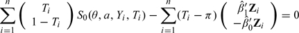
It has been shown via numerical studies that the ZTD performs well via the standard stepwise regression by ignoring the sampling variation of the estimated weights when the dimension of Z is not large with respect to n. However, it is not clear how the ZTD augmentation performs with a relatively high-dimensional covariate vector Z. It would be interesting to compare the ZTD and the new proposal with the PBC data. To this end, we implement ZTD augmentation procedure using (1) baseline covariates (p = 18); (2) baseline covariates and their quadratic transformations as well as all their two-way interactions (p = 178); and (3) only five baseline covariates: edema and log-transformed age, serum albumin, serum bilirubin, and standardized blood clotting time, which were selected in building a multivariate Cox regression model to predict the patient's survival by Therneau and Grambsch (2000). Note that the ZTD procedure augments the following estimating equations for θ₀:

where a_t0 is the restricted mean for the comparator and θ is the treatment difference, ${\stackrel{\sim }{\Delta }}_i=I(Y_{i}and{t}_0<C_i)$, and ${\widehat{K}}_j(·)$ is the Kaplan–Meier estimate for the survival function of censoring time C in group T = j,j = 0,1. In Table 3, we present the resulting ZDT point estimates and their corresponding standard error estimates for the above three cases. Here, we used the standard forward stepwise regression procedure to select the augmentation covariates with the entry Type I error rate of 0.10 (Zhang and others, 2008, Zhang and Gilbert, 2010). It appears that using the entire data set for selecting covariates and making inferences about θ₀ may introduce nontrivial bias and an overly optimistic standard error estimate when p is large. On the other hand, the new procedure does not lose efficiency and yields similar result as ZTD procedure when p is small.

Table 3.

Comparisons between the new and ZTD estimate with the data from the Mayo Clinic PBC clinical trial (SE: estimated standard error)

p	The new optimal procedure		ZTD
	Estimate	SE	Estimate	SE
5	92.0	121.5	96.3	119.4
18	106.3	121.4	126.4	111.7
178	110.1	122.6	65.3	114.6

BIAS, empirical bias; ESE, empirical standard error.

6. REMARKS

The new proposal performs well even when the dimension of the covariates involved for augmentation is not large. The new estimation procedure may be implemented for improving estimation precision regardless of the marginal distributions of the covariate vectors between two treatment groups being balanced. On the other hand, to avoid post ad hoc analysis, we strongly recommend that the investigators prespecify the set of all potential covariates for adjustment in the protocol or the statistical analysis plan before the data from the clinical study are unblinded.

The stratified estimation procedure for the treatment difference is also commonly used for improving the estimation precision using baseline covariate information. Specifically, we divide the population into K strata based on baseline variables, denoted by {Z∈B₁},…,{Z∈B_K}, the stratified estimator is

where ${\widehat{\theta }}_k$ and w_k are corresponding simple two sample estimator for the treatment difference and the weight for the kth stratum, k = 1,…,K. In general, the underlying treatment effect may vary across strata and consequently the stratified estimator may not converge to θ₀. If θ₀ is the mean difference between two groups and w_k is the size of the kth stratum, ${\widehat{\theta }}_{\text{str}}$ is a consistent estimator for θ₀. Like the ANCOVA, the stratified estimation procedure may be problematic. On the other hand, one may use the indicators {I(Z∈B₁),…,I(Z∈B_K)}^′ to augment $\widehat{\theta }$ to increase the precision for estimating the treatment difference θ₀.

In this paper, we follow the novel approach taken, for example, by Zhang and others (2008) for augmenting the simple two sample estimator but present a systematic practical procedure for choosing covariates for making valid inferences about the overall treatment difference. When p is large, there are several advantages over other approaches for augmenting $\widehat{\theta }$ with covariates. First, it avoids the complex variable selection step in two arms separately as proposed in Zhang and others (2008). Second, compared with other variable selection methods such as the stepwise regression, the lasso method directly controls the variability of $\widehat{\gamma },$ which improves the empirical performance of the augmented estimator. Third, the cross validation step enables more accurate estimation of the variance of the augmented estimator. When λ increases from 0 to + ∞, the resulting estimator varies from the fully augmented estimator using all the components of Z_i to $\widehat{\theta }.$ The lasso procedure also possesses superior computational efficiency with high-dimensional covariates to alternatives. Last, since ${\widehat{\theta }}_{\text{ZTD}}$ can also be viewed as a generalized method of moment estimator with

as moment conditions (Hall, 2005), the cross validation method introduced here may be extended to a much broader context than the current setting.

It is important to note that if a permuted block treatment allocation rule is used for assigning patients to the two treatment groups, the augmentation method proposed in the paper can be easily modified. For instance, for the K-fold cross validation process, one may choose the sets {𝒟_k,k = 1,…,K} so that each permuted block would not be in different sets.

For assigning patients to the treatment groups, a stratified random treatment allocation rule is also often utilized to ensure a certain level of balance between the two groups in each stratum. For this case, a weighted average θ₀ of the treatment differences θ_k0 with weight w_k,k = 1,…,K, across K strata may be the parameter of interest for quantifying an overall treatment contrast. Let ${\widehat{\theta }}_k$ be the simple two sample estimator for θ_k0 and ${\widehat{w}}_k$ be the corresponding empirical weight for w_k. Then the weight average $\widehat{\theta }={\sum }_k{\widehat{w}}_k{\widehat{\theta }}_k/{\sum }_k{\widehat{w}}_k$ is the simple estimator for θ₀. For the kth stratum, one may use the same approach as discussed in this paper to augment ${\widehat{\theta }}_k,$ let the resulting optimal estimator be denoted by ${\widehat{\theta }}_{\text{opt},k}.$ Then we can use the weighted average ${\sum }_k{\widehat{w}}_k{\widehat{\theta }}_{\text{opt},k}/{\sum }_k{\widehat{w}}_k$ to estimate θ₀. On the other hand, for the case with the dynamic treatment allocation rules (see, e.g., Pocock and Simon, 1975), it is not clear how to obtain a valid variance estimate even for the simple two sample estimator $\widehat{\theta }$ (Shao and others, 2010). How to extend the augmentation procedure to cases with more complicated treatment allocation rule warrants further research.

FUNDING

National Institutes of Health (R01 AI052817, RC4 CA155940, U01 AI068616, UM1 AI068634, R01 AI024643, U54 LM008748, R01 HL089778).

APPENDIX A

Asymptotical equivalence between ZTD and ANCOVA

When the group mean is the parameter of interest, the naive estimator for θ₀ can viewed as the root of the estimating equation

where a = E(Y|T = 0) is a nuisance parameter. In the ZTD augmentation procedure, one may augment this simple estimating equation via following steps:

• Obtain the initial estimator

  

from the original estimating equation

• Obtain ${\widehat{\beta }}_1$ and ${\widehat{\beta }}_0^{\prime }$ by minimizing the objective function

  

and

respectively. In other words, using ${\widehat{\beta }}_j^{\prime }\mathbf{Z}$ to approximate E{S₀(θ₀,a₀;Y,T)|Z,T = j}.

• Solve the augmented estimating equations

  

to obtain ${\widehat{\theta }}_{\text{ZTD}}$.

The resulting ${\widehat{\theta }}_{\text{ZTD}}$ is always asymptotically more efficient than the naive counterpart and a simple sandwich variance estimator can be used to consistently estimate the variance of the new estimator. It has been shown that ${\widehat{\theta }}_{\text{ZTD}}$ is asymptotically the most efficient one from the class of the estimators

whose members are all consistent for θ₀ and asymptotically normal. When π = 0.5

the optimal weight minimizing the variance of

is simply

Therefore, ${\widehat{\theta }}_{\text{ZTD}}$ is asymptotically equivalent to the commonly used ANCOVA estimator. This equivalence is noted in Tsiatis and others (2008).

APPENDIX B

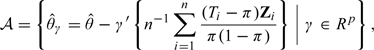
Justification of the cross validation based variance estimator for ${\widehat{\theta }}_{\text{cv}}\left(\lambda \right)$

To justify the cross validation based variance estimator, first consider the expansion

The variance of ${\widehat{\theta }}_{\text{cv}}\left(\lambda \right)$ can be expressed as V₁₁ + V₂₂ − 2V₁₂, where

and

First,

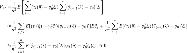Therefore, the variance of the augmented estimator ${\widehat{\theta }}_{\text{cv}}\left(\lambda \right)$ is approximately

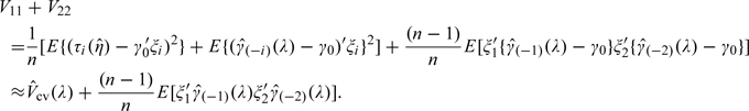In our experience, $d\left(\lambda \right)=E[{\xi }_1^{\prime }{\widehat{\gamma }}_{(-1)}\left(\lambda \right){\xi }_2^{\prime }{\widehat{\gamma }}_{(-2)}\left(\lambda \right)]=O(n^{-2})$ is very small compared with ${\widehat{V}}_{\text{cv}}\left(\lambda \right)=O(n^{-1})$ and is negligible, when λ is not close 0. Therefore, in general, ${\widehat{V}}_{\text{cv}}\left(\lambda \right)$ serves as a satisfactory estimator for the variance of ${\widehat{\theta }}_{\text{cv}}\left(\lambda \right).$ For small λ, to explicitly estimate d(λ), the covariance between ${\xi }_1^{\prime }{\widehat{\gamma }}_{(-1)}\left(\lambda \right)$ and ${\xi }_2^{\prime }{\widehat{\gamma }}_{(-2)}\left(\lambda \right)$, one may use

(6.1)

as an ad hoc jackknife-type estimator, where $\widehat{\gamma }\left(\lambda \right)$ is the lasso solution based on the entire data set. To justify the approximation, first note that when λ is close to 0,

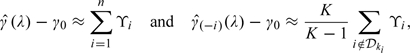where ϒ_i is the mean zero influence function from the ith observation for $\widehat{\gamma }\left(\lambda \right).$ Therefore,

which can be approximated by $\widehat{d}\left(\lambda \right)$ and one may use ${\widehat{V}}_{\text{cv}}\left(\lambda \right)+(n-1)\widehat{d}\left(\lambda \right)/n$ as the variance estimator for the augmented estimator. Note that the difference between ${\widehat{V}}_{\text{cv}}$ and its modified version appears to be negligible in all the numerical studies presented in the paper.

References

- Flemming T, Harrington D. Counting Processes and Survival Analysis. New York: Wiley; 1991. [Google Scholar]
- Gilbert PB, Sato M, Sun X, Mehrotra DV. Efficient and robust method for comparing the immunogenicity of candidate vaccines in randomized clinical trials. Vaccine. 2009;27:396–401. doi: 10.1016/j.vaccine.2008.10.083. [DOI] [PMC free article] [PubMed] [Google Scholar]
- Hall A. Generalized Method of Moments (Advanced Texts in Econometrics). London: Oxford University Press; 2005. [Google Scholar]
- Koch G, Tangen C, Jung J, Amara I. Issues for covariance analysis of dichotomous and ordered categorical data from randomized clinical trials and non-parametric strategies for addressing them. Statistics in Medicine. 1998;17:1863–1892. doi: 10.1002/(sici)1097-0258(19980815/30)17:15/16<1863::aid-sim989>3.0.co;2-m. [DOI] [PubMed] [Google Scholar]
- Leon S, Tsiatis A, Davidian M. Semiparametric efficiency estimation of treatment effect in a pretest-posttest study. Biometrics. 2003;59:1046–1055. doi: 10.1111/j.0006-341x.2003.00120.x. [DOI] [PubMed] [Google Scholar]
- Lu X, Tsiatis A. Improving efficiency of the log-rank test using auxiliary covariates. Biometrika. 2008;95:676–694. [Google Scholar]
- Pocock S, Simon R. Sequential treatment assignment with balancing for prognostic factors in the controlled clinical trial. Biometrics. 1975;31:102–115. [PubMed] [Google Scholar]
- Shao J, Yu X, Zhong B. A theory for testing hypotheses under covariate-adaptive randomization. Biometrika. 2010;97:347–360. [Google Scholar]
- Therneau T, Grambsch P. Modeling Survival Data: Extending the Cox Model. New York: Springer; 2000. [Google Scholar]
- Tibshirani R. Regression shrinkage and selection via the lasso. Journal of the Royal Statistical Society, Series B. 1996;58:267–288. [Google Scholar]
- Tsiatis A. Semiparametric Theory and Missing Data. New York: Springer; 2006. [Google Scholar]
- Tsiatis A, Davidian M, Zhang M, Lu X. Covariate adjustment for two-sample treatment comparisons in randomized clinical trials: a principled yet flexible approach. Statistics in Medicine. 2008;27:4658–4677. doi: 10.1002/sim.3113. [DOI] [PMC free article] [PubMed] [Google Scholar]
- Zhang M, Gilbert PB. Increasing the efficiency of prevention trials by incorporating baseline covariates. Statistical of Communications in Infectious Diseases. 2010;2 doi: 10.2202/1948-4690.1002. http://www.bepress.com/scid/vol2/iss1/art1. doi:10.2202/1948–4690.1002. [DOI] [PMC free article] [PubMed] [Google Scholar]
- Zhang M, Tsiatis A, Davidian M. Improving efficiency of inferences in randomized clinical trials using auxiliary covariates. Biometrics. 2008;64:707–715. doi: 10.1111/j.1541-0420.2007.00976.x. [DOI] [PMC free article] [PubMed] [Google Scholar]