Disparity-Tuned Population Responses from Human Visual Cortex

Abstract

We used source imaging of visual evoked potentials to measure neural population responses over a wide range of horizontal disparities (0.5–64 arcmin). The stimulus was a central disk that moved back and forth across the fixation plane at 2 Hz, surrounded either by binocularly uncorrelated dots (disparity noise) or by correlated dots presented in the fixation plane. Both disk and surround were composed of dynamic random dots to remove coherent monocular information. Disparity tuning was measured in five visual regions of interest (ROIs) [V1, human middle temporal area (hMT+), V4, lateral occipital complex (LOC), and V3A], defined in separate functional magnetic resonance imaging scans. The disparity tuning functions peaked between 2 and 16 arcmin for both types of surround in each ROI. Disparity tuning in the V1 ROI was unaffected by the type of surround, but surround correlation altered both the amplitude and phase of the disparity responses in the other ROIs. Response amplitude increased when the disk was in front of the surround in the V3A and LOC ROIs, indicating that these areas encode figure–ground relationships and object convexity. The correlated surround produced a consistent phase lag at the second harmonic in the hMT+ and V4 ROIs without a change in amplitude, while in the V3A ROI, both phase and amplitude effects were observed. Sensitivity to disparity context is thus widespread in visual cortex, but the dynamics of these contextual interactions differ across regions.

Introduction

In animals with frontal eyes, a percept of depth is produced by small horizontal disparities between the monocular half-images (Wheatstone, 1836). Disparity-sensitive neurons in primate striate cortex respond only to absolute disparity—the interocular difference in stimulus position (Cumming and Parker, 1999; Nienborg and Cumming, 2006; Parker, 2007). However, the responses of some disparity-sensitive neurons in extrastriate visual areas are affected by the presence of other disparities in the image and are therefore involved in encoding disparity differences (i.e., relative disparity) (Thomas et al., 2002; Umeda et al., 2007).

Extracellular recordings describe the activity of individual neurons but do not characterize population-level disparity responses that may be distributed over large cortical networks. Several recent studies have used functional magnetic resonance imaging (fMRI) to assay population-level disparity responses in human visual cortex (Mendola et al., 1999; Backus et al., 2001; Gilaie-Dotan et al., 2001; Tsao et al., 2003; Preston et al., 2008) to more complex three-dimensional (3D) relationships (Welchman et al., 2005; Chandrasekaran et al., 2007; Georgieva et al., 2009; Preston et al., 2009). Although these fMRI studies have been successful at localizing the neural correlates of depth perception in both the ventral and dorsal pathways of the visual system (Neri et al., 2004; Neri, 2005), little is known about the dynamics underlying these responses due to the slow coupling of the blood oxygen level-dependent (BOLD) signal to neural activity.

In this study, we combined high-density electroencephalogram (EEG) recording with MRI and fMRI functional area definitions to characterize the population-response dynamics that are evoked by periodically changing horizontal disparities. Using dynamic random-dot patterns, we moved a disparity-defined disk back and forth across the fixation plane and measured the EEG response as a function of the amplitude of the disparity modulation. To determine whether different areas respond selectively to absolute and relative disparity, we measured the response in the presence of two types of surround, one composed of binocularly uncorrelated disparity noise and the other composed of correlated dots with zero disparity. While it was impossible to eliminate all possible reference stimuli from our display, the noise surround effectively obscured all local references, so we call this condition the “absolute” disparity condition. The correlated surround provided a robust local reference system for the calculation of relative disparity—the relative disparity condition. Disparity tuning functions were measured in five regions of interest (ROIs) [V1, human middle temporal area (hMT+), V4, lateral occipital complex (LOC), and V3A]. We found that when the surround was uncorrelated, all five ROIs showed similar disparity tuning, with a peak at ∼8 arcmin. The correlated surround increased response amplitudes in the LOC and V3A ROIs, when the central disk was displayed in front of the background, implicating these ROIs in a cortical network specialized in the processing of convex objects. The phases of responses at the second harmonic were systematically delayed in the V3A, V4, and hMT+ ROIs in the correlated surround compared with the uncorrelated surround condition. This phase shift suggests that these ROIs may extract the relative disparity contained in the figure–ground relationship.

Materials and Methods

Subjects and stimuli.

Twelve subjects (8 males, 4 females) participated in this study. They all had normal or corrected-to-normal vision. Their informed consent was obtained before experimentation under a protocol that was approved by the Institutional Review Board of the Smith-Kettlewell Eye Research Institute.

Using dense dynamic random-dot patterns refreshed at f = 28.33 Hz (density of 30 dots by square degree of visual field), we modulated a disparity-defined central disk (5° diameter) at 2 Hz back and forth across the fixation plane. This frequency value was a tradeoff between low frequencies that permit a more reliable phase analysis and higher values that prevent subjects from following the disk disparity with convergence movements. The viewing distance was 70 cm (for a schematic drawing of the stimuli, see Fig. 1). Background luminance was 2.3 cd/m²; dot contrast was 89%.

Figure 1.

Description of the stimuli. a, Front view. The two half-images composed of dynamic random dots contained the same monocular information. In the first set of conditions, the dots in the annulus were uncorrelated. In the second set, the dots in the left eye matched with dots in the right eye, creating a static surround at zero disparity. b, 3D view of the fused half-images. The central disk moved back (at time t1= 0 ms) and forth (t2 = 250 ms). c, Top view. d, Front view.

In the first set of eight conditions, a 12° annulus consisting of uncorrelated dots (i.e., disparity noise) surrounded the modulating central disk. In this case, the only depth information available during a trial was the change in the absolute disparity of the dots defining the central disk. This disk was first presented back from the fixation plane at d arcmin (uncrossed disparity) for 250 ms and then in front of it (−d arcmin, crossed disparity) for 250 ms repeatedly for 11 s. The eight conditions comprised horizontal disparity values of ±0.5, ±1, ±2, ±4, ±8, ±16, ±32, and ±64. The average disparity of the stimulus during the period of presentation is zero and therefore minimized vergence demand. Nevertheless, we presented nonius lines and a fixation point before each 11 s trial to ensure that subjects were converged initially on the fixation plane.

To determine whether the absence of a fixation point produced a fixation bias during the disparity modulation, we performed an additional psychophysical nonius alignment test (McKee and Mitchison, 1988; Ukwade et al., 2003). For a set of 50 trials, the subject viewed the modulated disk surrounded by the uncorrelated noise. After each 11 s trial, he or she judged which of three vertical lines presented in the upper visual field of the left eye was aligned with a single vertical line in the lower visual field of the right eye. These measurements were repeated for two different spacings between the upper lines: 5.5 and 12 arcmin. Five subjects participated in these nonius tests. From these measurements, we concluded that vergence was stable and unbiased during the trial (supplemental Fig. 1, available at www.jneurosci.org as supplemental material).

In the second set of conditions, the central disk was modulated using the same eight values of disparity but was presented with a surround that consisted of correlated dots presented in the fixation plane (i.e., 0 disparity). This condition allowed us to determine the effect of relative disparity on the EEG response.

EEG signal acquisition and source imaging procedure acquisition.

The responses to the two stimulus configurations (i.e., disparity modulation with and without a correlated surround) were recorded independently. Stimuli were presented in trials that lasted 11 s; the first second of the record was discarded to avoid start-up transients. Trials for the eight disparity conditions were run interspersed in random order in blocks of 40 (5 trials per condition). The blocks were repeated four times, producing altogether a total of 20 trials (200 s) per condition.

The EEG was collected with 128-sensor HydroCell Sensor Nets (Electrical Geodesics) and was bandpass filtered from 0.1 to 200 Hz. Following each experimental session, the 3D locations of all electrodes and three major fiducials (nasion, left, and right periauricular points) were digitized using a 3Space Fastrack 3-D digitizer (Polhemus). For all subjects, the 3D digitized locations were used to coregister the electrodes to their T1-weighted anatomical MRI scans. Raw data were evaluated off-line according to a sample-by-sample thresholding procedure to remove noisy sensors that were replaced by the average of the six nearest spatial neighbors. Once noisy sensors were substituted, the EEG was re-referenced to the common average of all the sensors. Additionally, EEG epochs that contained a large percentage of data samples exceeding threshold (25–50 mV) were excluded on a sensor-by-sensor basis. Typically, these epochs were associated with eye movements or blinks.

Structural and functional magnetic resonance imaging.

Structural and fMRI scanning was conducted at 3T (Tim Trio, Siemens) using a 12-channel head coil. We acquired a T1-weighted MRI dataset (3D magnetization-prepared rapid acquisition gradient-echo (MP-RAGE) sequence, 0.8 × 0.8 × 0.8 mm³) and a 3D T2-weighted dataset (SE sequence at 1 × 1 × 1 mm³ resolution) for tissue segmentation and registration with the functional scans. For fMRI, we used a single-shot, gradient-echo echo planar imaging (EPI) sequence (repetition time, 2000 ms; echo time, 28 ms; flip angle, 80°; 126 volumes per run) with a voxel size of 1.7 × 1.7 × 2 mm³ (acquisition matrix, 128 × 128; field of view, 220 mm; bandwidth, 1860 Hz/pixel; echo spacing, 0.71 ms). We acquired 30 slices without gaps, positioned in the transverse-to-coronal plane approximately parallel to the corpus callosum and covering the whole cerebrum. Once per session, a two-dimensional SE T1-weighted volume was acquired with the same slice specifications as the functional series to facilitate registration of the fMRI data to the anatomical scan.

The FreeSurfer software package (http://surfer.nmr.mgh.harvard.edu) was used to perform gray and white matter segmentation and a mid-gray cortical surface extraction. This cortical surface had 20,484 isotropically spaced vertices and was used both as a source constraint and for defining the visual areas. The FreeSurfer package extracts both gray/white and gray/CSF boundaries, but these surfaces can have different surface orientations. In particular, the gray/white matter boundary has sharp gyri (the curvature changes rapidly) and smooth sulci (slowly changing surface curvature), while the gray matter/CSF boundary is the inverse, with smooth gyri and sharp sulci. To avoid these discontinuities, we generated a surface partway between these two boundaries that has gyri and sulci with approximately equal curvature.

Individual boundary element method conductivity models were derived from the T1- and T2-weighted MRI scans of each observer. The FSL toolbox (http://www.fmrib.ox.ac.uk/fsl/) was also used to segment contiguous volume regions for the scalp, outer skull, and inner skull, and to convert these MRI volumes into inner skull, outer skull, and scalp surfaces (Smith, 2002; Smith et al., 2004).

Visual area definition.

The general procedures for the scans used to define the visual areas (e.g., head stabilization and visual display system) are standard and have been described in detail previously (Brewer et al., 2005). Retinotopic field mapping defined ROIs for visual cortical areas V1, V2v, V2d, V3v, V3d, V3A, and V4 in each hemisphere (Tootell and Hadjikhani, 2001; Wade et al., 2002). ROIs corresponding to hMT+ were identified using low-contrast motion stimuli similar to those described by Huk and Heeger (2002).

The LOC was defined using a block-design fMRI localizer scan. During this scan, the observers viewed blocks of images depicting common objects (18 s/block) alternating with blocks containing scrambled versions of the same objects. The stimuli were those used in a previous study (Kourtzi and Kanwisher, 2000). The regions activated by these scans included an area lying between the V1/V2/V3 foveal confluence and the hMT+ that we identified as LOC. This definition covers almost all regions (e.g., V4d or LOC) that have previously been identified as lying within object-responsive lateral occipital cortex (Kourtzi and Kanwisher, 2000; Tootell and Hadjikhani, 2001).

Source imaging procedure.

An L2 minimum-norm inverse was computed with sources constrained to the location and orientation of the cortical surface (Dale and Sereno, 1993; Hämäläinen et al., 1993; Baillet et al., 2001). In addition, we modified the source covariance matrix in two ways to decrease the tendency of the minimum-norm procedure to place sources outside of the visual areas. These constraints involved the following: (1) increasing the variance allowed within the visual areas by a factor of two relative to other vertices; and (2) enforcement of a local smoothness constraint within an area using the first- and second-order neighborhoods on the mesh with a weighting function equal to 0.5 for the first order and 0.25 for the second order. The smoothness constraint therefore respects areal boundaries unlike other smoothing methods such as low-resolution brain electromagnetic tomography (LORETA) that apply the same rule throughout cortex (Pascual-Marqui et al., 1994).

ROI-based analysis of the steady-state visual-evoked potential.

In this study, we were mainly interested in the properties of the cortical responses in the frequency domain. The amplitudes associated with the even and odd harmonics of the stimulation frequencies reflect the symmetries and asymmetries in the response and therefore offer a unique view on the properties of the underlying neural populations (Regan, 1989; Vialatte et al., 2010). The corresponding phases provide information on the timing of the signals. We used a discrete Fourier transform to estimate the average response magnitude and phase associated with each functionally defined ROI of each subject (Appelbaum et al., 2006; Ales and Norcia, 2009).

Amplitude analysis.

We extracted the amplitudes of the dominant odd and even components of the 2 Hz stimulus frequency separately. The odd component was obtained by computing the root-mean-square value of the Fourier coefficients at the first and third harmonics (2 and 6 Hz, respectively). In a similar way, the even component was obtained from the Fourier coefficients of the second and fourth harmonics (4 and 8 Hz, respectively). To take into account the differences of noise levels between the recordings from each of our subjects (Vialatte et al., 2010), we computed the signal-to-noise ratio (SNR). We divided the root-mean-square values of the summed Fourier coefficients by those of an associated set of noise estimates, which were defined for a given frequency, f, by the average amplitude of the two neighbor frequencies [i.e., f − δf and f + δf, where δf is the frequency resolution of the Fourier analysis (0.5 Hz)]. For a given subject and a given frequency, the noise value was estimated from all the conditions belonging to the same recording session. The corresponding SNRs are presented in decibels (i.e., 20*log10).

In addition to the horizontal disparity tuning curves associated with the two types of surround, we also present the curves associated with the differences between the two sets. They were computed by subtracting the SNRs obtained for each horizontal disparity.

Statistical analysis of the amplitudes.

To determine whether the type of surround had a significant effect on the cortical responses, we performed statistical tests on the differences between the SNRs associated with the uncorrelated and correlated surrounds. As the tuning curve values were weaker and close to a baseline for the smallest and largest disparities (Figs. 2, 3), we grouped together the differences corresponding to disparities ranging from 2 to 16 arcmin for each visual ROI where the responses were more reliable. Because the SNRs are not normally distributed, we chose to use a nonparametric test: the Wilcoxon sign rank tests on the distributions. As we were making multiple comparisons (5 visual ROIs for 2 groups of harmonics), we used a Bonferroni correction and multiplied each p value by 10.

Figure 2.

Horizontal disparity tuning for the even harmonics. a, Locations of the different ROIs used in this study illustrated on one individual subject (lateral and ventral views). b, Global SNR responses averaged across subjects (in log units). The dotted lines represent the corresponding SEs. Both sets (with a correlated and an uncorrelated surround respectively) are presented on the top. The corresponding differences are displayed in the bottom. The star is associated with a p value of 0.05 (Wilcoxon test, Bonferroni corrected) for disparity values included in the 2–16 arcmin interval (emphasized by the cyan band). The corresponding equations of the linear models are displayed in blue.

Figure 3.

Horizontal disparity tuning at the odd harmonics. See Figure 2 for the details of the legend.

Phase analysis.

From the Fourier coefficients, we also obtained the phases associated with different ROIs. Newly developed techniques (Tolias et al., 2007; Berens et al., 2008) were used to calculate confidence intervals for the average value of our phase distributions (Zar, 1999, their Eqs. 26.23–26.26). We performed these computations using the circular statistics toolbox (Berens, 2009). As we were mainly interested in the phase delays/advances that may be introduced by the change in the surround, we grouped together the phases corresponding to disparities ranging from 2 to 16 arcmin, and computed the means and confidence intervals associated with each type of surround and their differences at the first and second harmonics (i.e., 2 and 4 Hz, respectively). This grouping allowed us to make our phase estimates more precise as the number of data points was multiplied by 4. Only the phases at the first and second harmonics were computed as it was not possible to obtain sufficient SNR for circular statistics at frequencies corresponding to the third and fourth harmonics (i.e., 6 and 8 Hz, respectively). To test whether the distributions corresponding to the differences were uniform, we performed Rayleigh tests (Fisher, 1995). We applied a Bonferroni correction that multiplied each raw p value by 10. To test whether differences existed between the ROIs, we performed a Watson–Williams test (Watson and Williams, 1956; Stephens, 1969), which is a circular analog of the one-factor ANOVA (Watson and Williams, 1956; Stephens, 1969). It tests the null hypothesis that all of the groups (i.e., in our case, the phase within the five visual ROIs) share a common direction.

Cross talk between the ROIs.

To demonstrate that our source reconstructions were not degraded by the imperfect spatial resolution of high-density EEG imaging, we performed simulations to estimate the independence of the signals obtained in each of the ROIs. This was calculated for each individual subject participating in the experiment by the following:

1. Simulating uniform activity within each of the areas defined by the independent fMRI measurements (i.e., the same amplitude was applied to all the cortical sources within a particular ROI). The extents of the fMRI-defined ROIs were comparable in size to the area of the visual stimulus;

2. Using the individual forward models to estimate the EEG topographies (see the Structural and functional magnetic resonance imaging section) corresponding to the different source distributions;

3. Estimating the average cortical activity (in absolute value) in each ROI using the inverse procedure described in the Source imaging procedure section; and

4. Comparing the levels of activity in a given ROI arriving there from each of the other ROIs to the activity generated within that ROI.

Results

Absolute disparity tuning: disparity tuning with the uncorrelated surround

We first describe the disparity tuning across ROIs for the uncorrelated surround condition, in which there is no disparity reference in the vicinity of the modulated disk. The SNR levels for the even harmonics as a function of disparity magnitude are shown in Figure 2. The even harmonics reflect the part of the total response that is equivalent after each repetitive shift (backward and forward) in the disparity of the central disk. The SNR in all five ROIs increases with increasing disparity to reach a peak between 2 and 16 arcmin, where its value ranges between 12 and 18 dB (corresponding to a linear factor between 4 and 8 times baseline). The function returns to its minimum response for disparities >32 arcmin.

The odd harmonics capture any asymmetry in the responses to crossed and uncrossed disparity or between shifts between the two signs of disparity. The responses at the odd harmonics also show a “U-shaped” tuning function in all five ROIs (Fig. 3). The presence of odd harmonics indicates that the response is stronger to one sign of disparity than the other, or to changes from one sign to the other.

To visualize the response asymmetry more clearly, an example temporal waveform is displayed in Figure 4. In this particular case, the responses (filtered to 20 Hz) correspond to stimulation at ±16 arcmin (the time courses associated to stimulation at ±2, ±4, and ±8 arcmin are provided in supplemental Fig. 2, available at www.jneurosci.org as supplemental material). The amplitude after the transition from uncrossed to crossed disparity is generally larger than the response after the transition from uncrossed to crossed disparity.

Figure 4.

Evoked response waveforms in the different ROIs (in microvolts) elicited by a disparity of 16 arcmin. The difference waveforms (blue) were obtained by subtracting for each subject sthe evoked responses associated with correlated and uncorrelated surround and averaging. The dotted lines give the SE. The time windows corresponding to the two perceptual states are indicated using different color codes: gray when the central disk is back from the fixation plan (uncrossed disparity at t1 = 0); and white when it is in front (crossed disparity at t2 = 250 ms).

It is possible that the asymmetrical responses are due to a convergence bias, as there were no fixation points or nonius lines present during the 11 s trial for the uncorrelated surround condition. However, psychophysical measurements of fixation stability showed that there was no bias in fixation (see the Subjects and stimuli section in Material and Methods) (supplemental Fig. 1, available at www.jneurosci.org as supplemental material). Moreover, we also obtained the same tuning function for the odd harmonics for the correlated surround condition, where nonius lines and a fixation point were present during the entire recording session.

Population model of the disparity tuning function

To better understand how our EEG-based measures of disparity tuning might relate to the properties of the underlying distribution of disparity-tuned cells, we computed predictions from several simple population models. The models differed in the distribution of receptive field sizes and corresponding disparity tuning widths, and in the number of cells at different disparity values.

All physiological studies indicate that there are many V1 neurons tuned to near zero disparities (Poggio et al., 1988; Cumming and DeAngelis, 2001; Prince et al., 2002). In Figure 5a, we have diagrammed the predicted envelope of the population response on the assumption that there is a large number of disparity-tuned neurons coding disparity out to ∼10 arcmin, each with a different peak disparity and with equal response levels. Beyond 10 arcmin, the number of cells decreases with increasing disparity, as indicated by Figure 5a (top left). To obtain the population response, we modeled the disparity tuning function of each neuron in the population as Gaussian because the EEG response is not sensitive to the phase of the underlying receptive fields (simulations with odd- and even-symmetric filters led to similar results). The output of each cell in the population was then summed for crossed and uncrossed disparity values on the initial assumption that the population response to crossed and uncrossed disparities is the same. The population response of this model is a monotonically decreasing tuning function, which is clearly unlike what we measured.

Figure 5.

a–c, Three models of the global tuning curves obtained from neural populations responding to different horizontal disparities. Each model is characterized by a sum of Gaussian functions whose number and SD can vary according to the disparity value (the “-” refers to crossed disparities). The distribution of these parameters is given by the three displays on the left in normalized units (n.u.). The top left and middle left panels give the neuron number. For visibility purposes, the decrease with the absolute value of the disparity (top left) and the bias between the crossed and uncrossed domain (middle left) are displayed separately. The left bottom panel gives the distribution of the SD of the disparity filters. The middle panel displays the associated tuning curves, and the right one displays the corresponding odd and even harmonics (both in normalized units). a, Assumes a decreasing number of disparity-tuned neurons with the absolute value of the disparity, but a uniform distribution of the receptive field sizes (i.e., of the SD) and no bias toward one of the domains. b, Adds an increase of the receptive field sizes with the disparity. c, Adds a bias toward the crossed disparity domain.

For >30 years, it has been thought that neurons coding large disparities have larger receptive fields than neurons coding small disparities—the size-disparity correlation (Felton et al., 1972; Marr and Poggio, 1979; Ohzawa et al., 1990; Prince et al., 2002). Neurons with larger receptive fields would necessarily give a larger response to extended random-dot displays than neurons with smaller receptive fields, even though there are probably more neurons tuned to zero than to larger disparities, since, at every spatial scale, there are neurons peaking at zero disparity (DeAngelis et al., 1991). The simulated population response with a large number of small disparities plus a symmetric population of cells with a size-disparity correlation is shown in Figure 5b. This response is tuned to mid-range disparities as are our measured data.

Any explanation for the shape of our tuning functions also needs to account for the asymmetric responses from crossed to uncrossed compared with uncrossed to crossed transitions. As we noted in discussing Figure 4, the temporal waveform shows that the response to crossed disparities is larger than the response to uncrossed disparities. In Figure 5c, we added a population bias of twice as many crossed vs uncrossed cells and computed a difference between the responses of crossed vs uncrossed cells in the population. This model produces the observed asymmetry.

Relative disparity tuning: tuning with the correlated surround

In the previous section, we referred to the responses to disparity modulation with an uncorrelated surround as being absolute disparity responses, because there was no immediate reference stimulus for the disparity-modulated disk, not even a fixation point. The edges of the computer monitors and/or equipment visible in the periphery might have provided a weak reference for the modulation, but the presence of disparity noise probably interfered with the relative disparity calculation. By contrast, a correlated annulus at zero disparity provides a strong reference disparity. Thus, the response with the correlated surround may reflect the contribution of relative disparity responses.

The green curves in Figures 2 and 3 show the tuning curves obtained in the presence of the correlated surround. It is apparent that the tuning functions for absolute and relative disparity are broadly similar. Both show an inverted U shape with a peak between 2 and 16 arcmin. Indeed, the even harmonics show little difference for the two surround conditions, except in V3A where there is a small, but significant (p < 0.05, Bonferroni corrected), increase in the SNR near the peak of the function. This enhanced response suggests that V3A is affected by the relative disparity differences in the stimulus. In addition, there are large and significant differences in the odd harmonics observed in the LOC and V3A ROIs. The significance of these increases was confirmed by the Wilcoxon tests (p < 0.01, Wilcoxon test, Bonferroni corrected). The differences in the LOC ROI seem to remain constant at a value ∼4 dB (∼58% increase), whereas in the V3A ROI the differential responses decrease from 7 to 2 dB with increasing disparity (Fig. 3, blue curves). To quantify these variations of the SNRs in this interval (i.e., 2–16 arcmin), we computed the best fitting linear models of the differential curves. The tuning in the LOC ROI was flat (slope, −0.1) but was steeper in the V3A ROI (slope, −0.3). These patterns agree with the findings of Preston et al. (2008). In their fMRI study, the LOC, unlike V3A, did not vary with increasing disparity. These results suggest that area V3A could encode the disparity magnitude, but LOC may encode only the spatial relationship (i.e., figure on ground) while performing a disparity-invariant object segmentation operation.

Population model of disparity response dynamics

To understand how different underlying populations of disparity-tuned cells might contribute to the differences in response waveforms/spectra we have observed, we developed a simple model of the evoked response and computed spectral distributions that were based on different assumptions about the population of underlying single-cell disparity tunings. The model assumed that two subpopulations participate in the response to our stimuli, one associated with uncrossed disparities (i.e., when the disk is behind the fixation plan) and the other with crossed disparities (i.e., when the disk is in front of the fixation plan). At the level of the EEG evoked response, the subpopulation responses are pooled linearly via volume conduction.

As noted above, the crossed response is always stronger than the uncrossed response for both surround conditions, and this difference in response is shown in Figure 6a. The asymmetric response waveform is shown at the top, and the component odd and even harmonic waveforms that give rise to it are shown beneath it. Our first question is how different variations in the underlying crossed and uncrossed populations could give rise the particular surround-dependent patterns of even and odd harmonics (response waveform) that we observed experimentally.

Figure 6.

Examples of hypothetical odd and even harmonic amplitude variations between two experimental conditions. a, EEG signal associated with two subpopulations for a given condition (top) and its normalized reconstruction from first- (middle) and second-harmonic (bottom) Fourier coefficients. The amplitudes were normalized according to the maximum value across the two frequencies. The central disk is behind the fixation plane between t1 (0 ms) and t2 (250 ms), and in front of it between t2 and t3 (500 ms). We used t3 = t1 to point out that the phase wraps around in steady-state stimulation. b, Variations of these amplitudes at the first and second harmonics between the uncorrelated and correlated surround conditions are indicated by the arrows. The time courses for the uncorrelated surround are presented in gray while those of the correlated surround are displayed in black. Reconstructions of the third and fourth harmonics are not shown for visibility purposes, but their characteristics may be easily deduced from the first and second harmonics. Amp., Amplitude; n.u., normalized units.

Figure 6b illustrates different predictions obtained from this model based on different changes in the subpopulation responses. The gray curves show the response to disparity modulation with the uncorrelated surround, and the black curves show the response with the correlated surround. We assumed that the time courses of the subpopulations can be simply modeled by two Gaussians (i.e., the response begins at zero, rises to a peak and then returns to zero when a given disparity is presented).

It is well known that human observers are more sensitive to relative changes than to absolute changes in disparity (Westheimer, 1979), so perhaps this enhanced sensitivity gives rise to a simple increase in response amplitude when the correlated surround is introduced. The first column of Figure 6b shows that an overall increase in the response amplitude will not reproduce our results, because an overall increase only increases the second harmonic, not the first.

In the second column of Figure 6b, we show what happens if the correlated surround enhances only the crossed response. Interestingly, this manipulation increases both the first and second harmonics. To produce an increase in only the first harmonic, there must be an increase in the crossed response and a corresponding decrease in the uncrossed response (Fig. 6b, third column).

Figure 6b does not illustrate all the possible configurations but focuses only on those that seem the most plausible for our study. In the V3A ROI, both the odd and even harmonics increase in the presence of the correlated surround (Fig. 6b, middle column). This pattern can be reproduced in our model by assuming that the response of only the crossed subpopulation is enhanced by the presence of a reference. Changes in the amplitude of the other state are possible but have to be negligible in comparison. In the LOC ROI, only the increase in the odd harmonics is statistically significant. This could mean that in this area, the surround inhibits the response of the uncrossed disparity and increases the responses from the crossed disparity (Fig. 6b, right column). However, this conclusion has to be tentative, because the absence of a statistically significant increase at the even harmonic does not mean that it does not exist, only that we could not measure it. In any case, our data suggest that the asymmetry between responses to crossed and uncrossed disparities is more pronounced in the LOC ROI than in the V3A ROI. These effects are apparent in the differential time courses (Fig. 4, blue curves; supplemental Fig. 2, blue curves, available at www.jneurosci.org as supplemental material).

Effect of surround disparity on response phase

The phase values associated with the first and second harmonics of the steady-state stimulation are displayed in Figures 7 and 8 as Nyquist plots. In most cases, it was possible to define a 95% confidence interval for the average difference (the only exception being LOC at the first harmonic).

Figure 7.

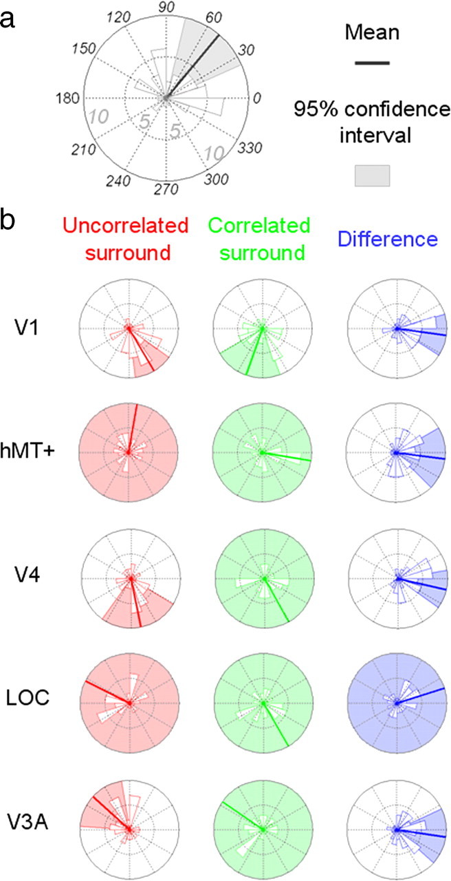
Histograms of the phases at the first harmonic (i.e., f = 2 Hz) for disparity ranging from 2 to 16 arcmin (12 subjects). Each small graphic displays the distribution of the 48 corresponding data points. a, Phases are presented in degrees on the trigonometric circle (anticlockwise progression). The number of data points included in each portion of the histograms is provided by the radius of the wedges. The inner and outer circles correspond to 5 and 10 data points, respectively. The thick lines give the means of the distributions, and the shadowed portions outline the 95% confidence interval for these means. The histograms lacking colored wedges refer to phases whose confidence intervals cannot be reliably estimated. b, Phases of the different ROIs for the uncorrelated and correlated surround (in red and green, respectively). The difference (i.e., correlated − uncorrelated) is displayed in blue.

Figure 8.

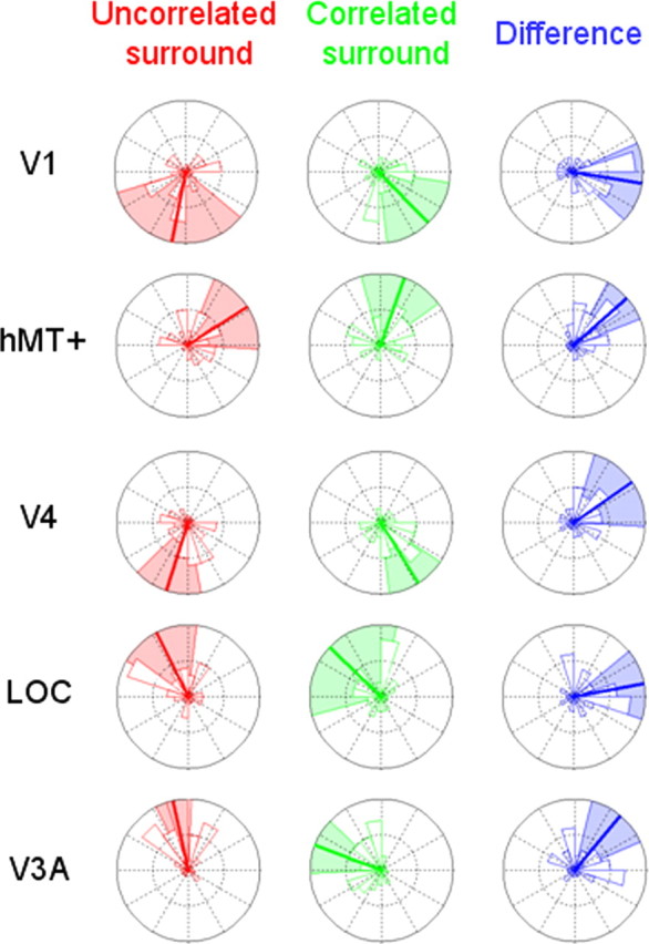
Histograms of the 12 subject phases at the second harmonic (i.e., 2f = 4 Hz) for disparity ranging from 2 to 16 arcmin. See Figure 6 for the details of the display.

At the first harmonic (Fig. 7), the phase difference between uncorrelated and correlated surround conditions are on average about zero (although a confidence interval could not be estimated for the LOC ROI). At the second harmonic, the V1 and LOC ROIs also have an average difference of approximately zero (Fig. 8). Areas hMT+, V4, and V3A show, however, a different behavior as reliable phase lags are obtained. The hMT+ phase difference is 41.6° on average and its 95% confidence interval is 21.46–61.76°. The V4 phase is 34.93° on average (95% confidence interval, −2.94 to 72.8°), and theV3A phase is 50° on average (95% confidence interval, 23.85–76.12°). These phase differences are consistent with either lags of ∼30 ms or leads of ∼220 ms. Given the time intervals, it seems more plausible that they are lags than leads.

The phase histograms suggest that even when averaged across subjects, the distributions of the phases are centered on specific values in different ROIs. These results were mainly confirmed by Rayleigh tests where the corrected p values at the first harmonic for the V1, hMT+, V4, LOC, and V3A ROIs were equal to 2.8e-4, 0.055, 5e-5, 2 and 0.021, respectively; the corrected p values for the second harmonic were 0.017, 2.7e-6, 0.066, 0.003, and 7.4e-4, respectively. The Watson–Williams test also demonstrated that there was a statistically significant main effect of the ROI at the second harmonic (the null hypothesis is rejected with p = 0.0036) but not at the first harmonic (p = 0.7252).

From the phases within the V1 and LOC ROIs, we can conclude that the correlated surround does not introduce changes in the dynamics of these areas. To characterize the results obtained in the other ROIs (i.e., phase lags at the second harmonic, but not at the first), we used the model shown in Figure 6 to explore how changing the timing of the subpopulations in different ways changes the global response waveform and the phase of the different harmonic components. We assume that the surround induces a time delay in either one (either the smallest amplitude population or the largest) or both of the subpopulations. Figure 9 displays the associated variations in the phases at the first and second harmonics. The time delay used in Figure 9 (Δt = 30 ms) corresponds to a phase lag of ∼45° at 4 Hz and is therefore in the ballpark of the values obtained in areas V3A, hMT+, and V4.

Figure 9.

Model of the odd and even harmonic phase variations between two experimental conditions. a, EEG signals associated with two subpopulations for a given condition (top) and its normalized reconstructions from its Fourier coefficients at the first (middle) and second harmonic (bottom). See Figure 6 for the details of the display. b, Effect of a time delay in the processing on the phase. Three different possibilities are examined. In the first one (b, left column), the correlation in the surround induces a delay of ∼30 ms (equivalent to a phase lag of 45° at 4 Hz) only when the disk is in front of the fixation plane. This results in equivalent phase lags at both the first and second harmonics. In the second one (b, middle column), both uncrossed and crossed disparities are affected by the correlated surround, and phase lags appear at the first and second harmonics with a phase lag twice as large in the second harmonic. In the last one (b, right column), only the response to the crossed disparity are delayed, and both the first and second harmonics contain a phase lag with a more important value for the first one. Amp., Amplitude; n.u., normalized units.

Any delay leads to a phase shift at the second harmonic. However, when only one of the subpopulations is affected, this phase shift is also present at the first harmonic with a value that is either equal when only the smaller subpopulation is affected (Fig. 9b, three left panels) or greater when only the larger amplitude subpopulation is affected (Fig. 9b, three right panels). When both subpopulations are delayed, the phase lag at the first harmonic still occurs but is half the size of the lag at the second harmonic. Although our data indicate that there is no phase lag at the first harmonic, the confidence level surrounding the estimated lag is large, so a small phase lag may be buried in the noise.

Our data are certainly more likely to correspond to this last model (Fig. 9b, column 2), which therefore suggests that the effects obtained may be associated with a time delay that would affect both the two subpopulations responding to crossed and uncrossed disparity (or to the transition between them).

Resolution of source-imaged steady-state visual-evoked potential

Source imaging with high-density EEG recordings allows the estimation of the current density at different, well defined cortical locations in individual subjects. However, dispersion of the electric field by the head volume smoothes the electrode signals, making it difficult to precisely estimate their cortical origins. The L2 minimum norm reconstruction approach we applied in our study is related to similar techniques whose localization errors range <10 mm (see Baillet et al., 2001; Bai et al., 2007) for the EEG. These techniques have been successful in reconstructing the retinotopic properties of early visual areas (Im et al., 2007; Sharon et al., 2007; Hagler et al., 2009). Given that the Euclidean distance between the cortical areas used in our study is at least 2 cm (except between ROIs hMT+ and LOC), the resolution of the inverse should be sufficient to resolve responses in the areas that we have chosen. However, to characterize the accuracy of our estimates, we have calculated a “cross-talk” matrix (see the Cross talk section in Materials and Methods). For each ROI, this matrix show how much activity is picked up in a given ROI from activity in each of the other ROIs. The cross-talk magnitude is referenced to activity originating in the ROI where the cross talk is being estimated. Figure 10 provides the average interarea cross talk obtained from our 12 subjects. The visual areas used in the analysis are grouped together within the white dotted line region. Areas V2 and V3, which were excluded from the analysis are also presented outside this region for comparison.

Figure 10.

Theoretical estimates of cross talk between source-imaged EEG signals in retinotopically defined visual areas. Grayscale values at row i and column j represent the relative contribution of area j to the cortical current density estimate in area i. Individual definitions from seven different areas (V1, hMT+, V4, LOC, V3A, V2, and V3) are included. The ROIs used in the study are grouped together within the white dotted line region. Areas V2 and V3, which were excluded from the analysis are also presented for comparison.

Values at row i and column j represent the relative contribution of area j to the cortical current density estimate in area i. The normalization is obtained by dividing by the amplitude obtained in area i when only area i was activated in the simulation set. For example, when we estimated the activity in V1, the absolute amplitudes obtained from hMT+, V4, LOC, and V3A when they were simulated independently (i.e., the second, third, fourth, and fifth columns of the first line of the cross-talk matrix) were respectively 12.39, 10.25, 14.11, and 30.33% of the amplitude in V1 when only V1 was activated (i.e., first line, first column). An ideal estimation of the cortical current densities would lead to zero cross talk, and the associated matrix would be equal to the identity. In our study however, hMT+, LOC, and V3A received on average <30% cross talk from other areas. V4 has higher cross talk, but it is <60% of its own activity. Note that coactivations from hMT+, V4, LOC, and V3A together would not equal a linear summation of their individual contributions as significant cancellations could arise between them (Ahlfors et al., 2010). We excluded areas and V2 and V3 because they pick up large amounts of cross talk from the other areas (Fig. 10, outer rows and columns).

We find that the V1 ROI receives only marginal contributions from most other areas, with the largest contribution coming from area V3A (30% relative to the strength of V1 itself). One major result of our study is that V3A responses are affected by the nature of the surround, whereas V1 responses are not. If V1 tuning functions were corrupted by area V3A, we should have measured this effect in V1 as well. The absence of such an effect suggests that our estimates of activity in V1 are not influenced significantly by our other ROIs. Using the same logic, area hMT+ mainly receives extraneous signals from LOC (40%), but its amplitude is not sensitive to the nature of the surround. The LOC ROI has its largest cross-talk inputs from V1 (33%) and hMT+ (32%), but we find a large surround correlation effect in this ROI at the odd harmonics, unlike V1 and hMT+. Although V3A receives a substantial potential contribution from V1 (45%), the difference in the responses of these two areas to the uncorrelated and correlated surrounds reveals that the response attributed to V3A is dominated by its own activity (see the blue curves in Figs. 2, 3). The cross-talk analysis shows that V4 is undoubtedly affected by V1 and V3A activity. However, unlike V1, the nature of the surround affects the phase of V4 response (although the corrected p value associated with the Rayleigh test is only 0.066). In addition, the SNRs in V4 are clearly different from those estimated in V3A, which suggests that the activity attributed to V4 is largely independent of previous activity.

Although we have estimated the probable contribution of cross talk among our chosen ROIs, one could argue that errors in our estimates may also come from cortical regions that are not included in this simulation. Given the nature of the EEG signals, these errors would be more likely to come from nearby regions (Im et al., 2007). In this context, V1 is completely surrounded by the other areas in the cross-talk matrix, yet V2 and V3 have only a marginal influence on it (26.46 and 14.6%, respectively) (Fig. 10). Because LOC and hMT+ are defined by thresholding the BOLD responses obtained from functional localizers, other areas near their border may have similar functional properties, including their response to disparity that may contribute to activity in these ROIs. Similarly, V4 activity may be partially dependent of other ventral regions such as VO-1 or VO-2 (Brewer et al., 2005). Finally, the effects we attribute to V3A could be due to dorsal areas V3B and V7 (Larsson and Heeger, 2006) that we did not define, although we note that our simulation indicates that the contribution from V3, which is also quite close, is only 23.5%.

As a final check on the robustness of our results against differences in the spatial extent of the ROI definitions, we defined a new version of the visual areas where the visual field extents were limited to 2.5° in radius, the same size as the figure region of our display (see supplemental Fig. 3, available at www.jneurosci.org as supplemental material). The results were very similar to those with the larger ROI extents used in the main analysis. Cross talk coming to areas V2 and V3 was increased slightly (e.g., inputs from V1 were 14.65 and 20% larger than with our initial definition of the ROIs), but the overall cross-talk error across the five ROIs actually used in our study remain unchanged (on average, they were decreased by 0.22%).

Discussion

We used steady-state EEG recordings to measure the population response in five visual ROIs (V1, hMT+, V4, LOC, and V3A) to a large disparity-modulated disk composed of dynamic random dots. The response to the disparity modulation increased with increasing disparity and then decreased at larger disparity values, producing an inverted U-shaped function that peaked at ∼8 arcmin. The tuning function in all five ROIs was similar. This result suggests that disparity tuning in extrastriate areas is largely inherited from the disparity-tuned population in V1. Our disparity tuning functions resemble those from other assays of the population disparity response, including psychophysical estimates (McKee et al., 1997), fMRI estimates (Backus et al., 2001), and early visual-evoked potential estimates that used a low channel count (Norcia et al., 1985). It is well known that at large disparities (>1.0°), human observers cannot discriminate whether a disparity-defined figure embedded in a dense random-dot display is in front or behind the reference plane (Glennerster, 1998). Prince et al. (2002) showed that this limit is consistent with the total range of responses of V1 neurons to random-dot displays. Thus, the decrease in the population response at large disparities undoubtedly arises from the scarcity of neurons coding large disparities in the central visual field.

At small disparities, the weaker values we obtained are in agreement with the predictions made by Backus et al. (2001) from single-cell recordings in V1 (Prince et al., 2002). This reflects the well known size-disparity correlation property of disparity-sensitive cells (Felton et al., 1972; Marr and Poggio, 1979; Ohzawa et al., 1990; Prince et al., 2002). Small receptive fields tuned near zero have high precision for detecting disparity modulation, but their small fields, confined to the central fovea, will produce less activity in response to extended region of disparity modulation, than the cells with large receptive tuned to large disparities.

Our evoked responses contained substantial energy at odd harmonics of the stimulus frequency. Because our stimulus was symmetric in terms of disparity, the presence of odd harmonics in the response indicates an asymmetry in the population response to equal crossed and uncrossed disparities. There is considerable evidence in the literature for a bias favoring crossed disparities. For example, psychophysical studies showed that the orientation of a Landolt C was more easily detected when presented in front of an interfering annulus than behind it (Lehmkuhle and Fox, 1980; Fox and Patterson, 1981). This general preference for crossed disparities has also been found in macaque V1 (Prince et al., 2002), V3 (Adams and Zeki, 2001), V4 (Watanabe et al., 2002; Hinkle and Connor, 2005; Tanabe et al., 2005), and MT/V5 (DeAngelis and Uka, 2003). A bias favoring crossed disparities in fMRI measurements has been seen in a large set of ROIs including LOC, hMT+, V4, and V3A (Preston et al., 2008).

Our very simple population model (Fig. 5) showed that a combination of three well known properties of disparity-tuned cells—limited disparity range, size-disparity correlation, and a bias for crossed disparities—produces a population disparity tuning function that is in substantial agreement with our measured data.

Relative disparity sensitivity

To determine whether any of our areas were potentially responsive to relative disparity, we compared the disparity tuning functions obtained with two different annular surrounds, a binocularly uncorrelated surround (disparity noise) and a correlated surround presented continuously at zero disparity (a reference stimulus). Because dynamic random-dot stereograms contain no monocular cues, this change in the surround correlation only alters the disparity field and introduces a zero disparity reference plane around the modulating center. The tagged response to changing disparity in the center region can thus be used to read out the influence of surrounding disparities on the population that is driven by the changing disparity.

Only the V1 responses were unaffected by relative/surround disparity, which is consistent with the observation from Cumming and Parker (1999), who found that neurons in V1 were selective only for absolute disparity. All extrastriate visual areas contain neurons that respond to relative disparity, beginning in area V2 (Thomas et al., 2002). Our results show that the correlated surround increases the response amplitude in LOC and V3A ROIs, and alters the temporal characteristics in areas hMT+, V3A, and V4. Our analysis of the pattern of increases in the odd and even harmonics suggests that the surround selectively increases the response to crossed disparities in the V3A and LOC ROIs. Other studies have shown that these areas respond preferentially to disparity-defined convexity and to figures presented in front of a surface (Mendola et al., 1999; Gilaie-Dotan et al., 2001; Preston et al., 2008; Vinberg and Grill-Spector, 2009). In addition to confirming this crossed preference, our modeling of the odd and even harmonics suggests that the surround decreases the uncrossed response in a push-pull fashion (Fig. 6) in the LOC ROI.

While it has been suggested that area MT responds primarily to absolute disparity (Neri, 2005)—a reasonable idea given its likely role in the network that generates convergence movements—there is also evidence that some MT neurons respond to disparity gradients (Nguyenkim and DeAngelis, 2003). Moreover, Chandrasekaran et al. (2007) found a strong correlation between their fMRI measurements of the BOLD response in hMT+ and psychophysical performance in a shape discrimination task for disparity-defined figures. Several articles have demonstrated that monkey V4 neurons are influenced by the relative disparity of the stimulus (Tanabe et al., 2004, Umeda et al., 2007), and similar results were obtained in a human study based on adaptation (Neri et al., 2004). Finally, in both humans and monkeys, area V3A has been shown to be involved in the processing of relative disparity (Backus et al., 2001; Tsao et al., 2003; Preston et al., 2008). Our results suggest that the calculation of relative disparity takes additional time in V3A, hMT+, and V4. It would be interesting to explore what accounts for this delay in future neurophysiological studies of the temporal response to disparity.

Admittedly, our imaging approach does not match the spatial resolution of fMRI. However, it does reveal aspects of visual processing that are not readily accessible from fMRI. For example, the most plausible explanation for the phase shifts in our data are that the calculation of relative disparity delays the population response in some visual areas. Furthermore, our frequency analysis demonstrated that in some areas, relative disparity enhances the response of crossed disparity more than uncrossed disparity and suggested that this asymmetrical effect is the basis of enhanced disparity sensitivity in the presence of a reference stimulus.

We have indicated the spatial uncertainty of EEG source imaging relative to fMRI by referring to activity as having arisen from “the V3A ROI” rather than “from V3A.” Our ROIs each have clear operational definitions, so referring to them in this way is valid. Our cross-talk analysis indicates that activity in these ROIs is strongly, but not completely, due to activity generated in the corresponding visual area.

References

- Adams DL, Zeki S. Functional organization of macaque V3 for stereoscopic depth. J Neurophysiol. 2001;86:2195–2203. doi: 10.1152/jn.2001.86.5.2195. [DOI] [PubMed] [Google Scholar]
- Ahlfors SP, Han J, Lin FH, Witzel T, Belliveau JW, Hämäläinen MS, Halgren E. Cancellation of EEG and MEG signals generated by extended and distributed sources. Hum Brain Mapp. 2010;31:140–149. doi: 10.1002/hbm.20851. [DOI] [PMC free article] [PubMed] [Google Scholar]
- Ales JM, Norcia AM. Assessing direction-specific adaptation using the steadystate visual evoked potential: results from EEG source imaging. J Vis. 2009;9:8. doi: 10.1167/9.7.8. [DOI] [PubMed] [Google Scholar]
- Appelbaum LG, Wade AR, Vildavski VY, Pettet MW, Norcia AM. Cue-invariant networks for figure and background processing in human visual cortex. J Neurosci. 2006;26:11695–11708. doi: 10.1523/JNEUROSCI.2741-06.2006. [DOI] [PMC free article] [PubMed] [Google Scholar]
- Backus BT, Fleet DJ, Parker AJ, Heeger DJ. Human cortical activity correlates with stereoscopic depth perception. J Neurophysiol. 2001;86:2054–2058. doi: 10.1152/jn.2001.86.4.2054. [DOI] [PubMed] [Google Scholar]
- Bai X, Towle VL, He EJ, He B. Evaluation of cortical current density imaging methods using intracranial electrocorticograms and functional MRI. Neuroimage. 2007;35:598–608. doi: 10.1016/j.neuroimage.2006.12.026. [DOI] [PMC free article] [PubMed] [Google Scholar]
- Baillet SM, Mosher JC, Leahy RM. Electromagnetic brain mapping. IEEE Signal Process Mag. 2001;18:14–30. [Google Scholar]
- Berens P. CircStat: a MATLAB toolbox for circular statistics. J Stat Softw. 2009;31:1–21. [Google Scholar]
- Berens P, Keliris GA, Ecker AS, Logothetis NK, Tolias AS. Comparing the feature selectivity of the gamma-band of the local field potential and the underlying spiking activity in primate visual cortex. Front Syst Neurosci. 2008;2:2. doi: 10.3389/neuro.06.002.2008. [DOI] [PMC free article] [PubMed] [Google Scholar]
- Brewer AA, Liu J, Wade AR, Wandell BA. Visual fields maps and stimulus selectivity in human ventral occipital cortex. Nat Neurosci. 2005;8:1102–1109. doi: 10.1038/nn1507. [DOI] [PubMed] [Google Scholar]
- Chandrasekaran C, Canon V, Dahmen JC, Kourtzi Z, Welchman AE. Neural correlates of disparity-defined shape discrimination in the human brain. J Neurophysiol. 2007;97:1553–1565. doi: 10.1152/jn.01074.2006. [DOI] [PubMed] [Google Scholar]
- Cumming BG, DeAngelis GC. The physiology of stereopsis. Annu Rev Neurosci. 2001;24:203–238. doi: 10.1146/annurev.neuro.24.1.203. [DOI] [PubMed] [Google Scholar]
- Cumming BG, Parker AJ. Binocular neurons in V1 of awake monkeys are selective for absolute, not relative, disparity. J Neurosci. 1999;19:5602–5618. doi: 10.1523/JNEUROSCI.19-13-05602.1999. [DOI] [PMC free article] [PubMed] [Google Scholar]
- Dale AM, Sereno MI. Improved localization of cortical activity by combining EEG and MEG with MRI cortical surface reconstruction: a linear approach. J Cogn Neurosci. 1993;5:162–176. doi: 10.1162/jocn.1993.5.2.162. [DOI] [PubMed] [Google Scholar]
- DeAngelis GC, Uka T. Coding of horizontal disparity and velocity by MT neurons in the alert macaque. J Neurophysiol. 2003;89:1094–1111. doi: 10.1152/jn.00717.2002. [DOI] [PubMed] [Google Scholar]
- DeAngelis GC, Ohzawa I, Freeman RD. Depth is encoded in the visual cortex by a specialized receptive field structure. Nature. 1991;352:156–159. doi: 10.1038/352156a0. [DOI] [PubMed] [Google Scholar]
- Felton TB, Richards W, Smith RA., Jr Disparity processing of spatial frequencies in man. J Physiol. 1972;225:349–362. doi: 10.1113/jphysiol.1972.sp009944. [DOI] [PMC free article] [PubMed] [Google Scholar]
- Fisher NI. Statistical analysis of circular data, revised edition. Cambridge, UK: Cambridge UP; 1995. [Google Scholar]
- Fox R, Patterson R. Depth separation and lateral interference. Percept Psychophys. 1981;30:513–520. doi: 10.3758/bf03202004. [DOI] [PubMed] [Google Scholar]
- Georgieva S, Peeters R, Kolster H, Todd JT, Orban GA. The processing of three-dimensional shape from disparity in the human brain. J Neurosci. 2009;29:727–742. doi: 10.1523/JNEUROSCI.4753-08.2009. [DOI] [PMC free article] [PubMed] [Google Scholar]
- Gilaie-Dotan S, Ullman S, Kushnir T, Malach R. Shape-selective stereo processing in human object-related visual areas. Hum Brain Mapp. 2002;15:67–79. doi: 10.1002/hbm.10008. [DOI] [PMC free article] [PubMed] [Google Scholar]
- Glennerster A. dmax for stereopsis and motion in random dot displays. Vision Res. 1998;38:925–935. doi: 10.1016/s0042-6989(97)00213-7. [DOI] [PubMed] [Google Scholar]
- Hagler DJ, Jr, Halgren E, Martinez A, Huang M, Hillyard SA, Dale AM. Source estimates for MEG/EEG visual evoked responses constrained by multiple, retinotopically mapped stimulus locations. Hum Brain Mapp. 2009;30:1290–1309. doi: 10.1002/hbm.20597. [DOI] [PMC free article] [PubMed] [Google Scholar]
- Hämäläinen M, Hari R, Ilmoniemi R, Knuutila J, Lounasmaa O. Magnetoencephalography: theory, instrumentation and applications to the non invasive study of human brain function. Rev Mod Phys. 1993;65:413–497. [Google Scholar]
- Hinkle DA, Connor CE. Quantitative characterization of disparity tuning in ventral pathway area V4. J Neurophysiol. 2005;94:2726–2737. doi: 10.1152/jn.00341.2005. [DOI] [PubMed] [Google Scholar]
- Huk AC, Heeger DJ. Pattern-motion responses in human visual cortex. Nat Neurosci. 2002;5:72–75. doi: 10.1038/nn774. [DOI] [PubMed] [Google Scholar]
- Im CH, Gururajan A, Zhang N, Chen W, He B. Spatial resolution of EEG cortical source imaging revealed by localization of retinotopic organization in human primary visual cortex. J Neurosci Methods. 2007;161:142–154. doi: 10.1016/j.jneumeth.2006.10.008. [DOI] [PMC free article] [PubMed] [Google Scholar]
- Kourtzi Z, Kanwisher N. Cortical regions involved in perceiving object shape. J Neurosci. 2000;20:3310–3318. doi: 10.1523/JNEUROSCI.20-09-03310.2000. [DOI] [PMC free article] [PubMed] [Google Scholar]
- Larsson J, Heeger DJ. Two retinotopic visual areas in human lateral occipital cortex. J Neurosci. 2006;26:13128–13142. doi: 10.1523/JNEUROSCI.1657-06.2006. [DOI] [PMC free article] [PubMed] [Google Scholar]
- Lehmkuhle S, Fox R. Effect of depth separation on metacontrast masking. J Exp Psychol Hum Percept Perform. 1980;6:605–621. doi: 10.1037//0096-1523.6.4.605. [DOI] [PubMed] [Google Scholar]
- Marr D, Poggio T. A computational theory of human stereo vision. Proc R Soc Lond B Biol Sci. 1979;204:301–328. doi: 10.1098/rspb.1979.0029. [DOI] [PubMed] [Google Scholar]
- McKee SP, Mitchison GJ. The role of retinal correspondence in stereoscopic matching. Vision Res. 1988;28:1001–1012. doi: 10.1016/0042-6989(88)90077-6. [DOI] [PubMed] [Google Scholar]
- McKee SP, Watamaniuk SN, Harris JM, Smallman HS, Taylor DG. Is stereopsis effective in breaking camouflage for moving targets? Vision Res. 1997;37:2047–2055. doi: 10.1016/s0042-6989(96)00330-6. [DOI] [PubMed] [Google Scholar]
- Mendola JD, Dale AM, Fischl B, Liu AK, Tootell RB. The representation of illusory and real contours in human cortical visual areas revealed by functional magnetic resonance imaging. J Neurosci. 1999;19:8560–8572. doi: 10.1523/JNEUROSCI.19-19-08560.1999. [DOI] [PMC free article] [PubMed] [Google Scholar]
- Neri P. A stereoscopic look at visual cortex. J Neurophysiol. 2005;93:1823–1826. doi: 10.1152/jn.01068.2004. [DOI] [PubMed] [Google Scholar]
- Neri P, Bridge H, Heeger DJ. Stereoscopic processing of absolute and relative disparity in human visual cortex. J Neurophysiol. 2004;92:1880–1891. doi: 10.1152/jn.01042.2003. [DOI] [PubMed] [Google Scholar]
- Nguyenkim JD, DeAngelis GC. Disparity-based coding of three-dimensional surface orientation by macaque middle temporal neurons. J Neurosci. 2003;23:7117–7128. doi: 10.1523/JNEUROSCI.23-18-07117.2003. [DOI] [PMC free article] [PubMed] [Google Scholar]
- Nienborg H, Cumming BG. Macaque V2 neurons, but not V1 neurons, show choice-related activity. J Neurosci. 2006;26:9567–9578. doi: 10.1523/JNEUROSCI.2256-06.2006. [DOI] [PMC free article] [PubMed] [Google Scholar]
- Norcia AM, Sutter EE, Tyler CW. Electrophysiological evidence for the existence of coarse and fine disparity mechanisms in human. Vision Res. 1985;25:1603–1611. doi: 10.1016/0042-6989(85)90130-0. [DOI] [PubMed] [Google Scholar]
- Ohzawa I, DeAngelis GC, Freeman RD. Stereoscopic depth discrimination in the visual cortex: neurons ideally suited as disparity detectors. Science. 1990;249:1037–1041. doi: 10.1126/science.2396096. [DOI] [PubMed] [Google Scholar]
- Parker AJ. Binocular depth perception and the cerebral cortex. Nat Rev Neurosci. 2007;8:379–391. doi: 10.1038/nrn2131. [DOI] [PubMed] [Google Scholar]
- Pascual-Marqui RD, Michel CM, Lehmann D. Low resolution electromagnetic tomography: a new method for localizing electrical activity in the brain. Int J Psychophysiol. 1994;18:49–65. doi: 10.1016/0167-8760(84)90014-x. [DOI] [PubMed] [Google Scholar]
- Poggio GF, Gonzalez F, Krause F. Stereoscopic mechanisms in monkey visual cortex: binocular correlation and disparity selectivity. J Neurosci. 1988;8:4531–4550. doi: 10.1523/JNEUROSCI.08-12-04531.1988. [DOI] [PMC free article] [PubMed] [Google Scholar]
- Preston TJ, Li S, Kourtzi Z, Welchman AE. Multivoxel pattern selectivity for perceptually relevant binocular disparities in the human brain. J Neurosci. 2008;28:11315–11327. doi: 10.1523/JNEUROSCI.2728-08.2008. [DOI] [PMC free article] [PubMed] [Google Scholar]
- Preston TJ, Kourtzi Z, Welchman AE. Adaptive estimation of three-dimensional structure in the human brain. J Neurosci. 2009;29:1688–1698. doi: 10.1523/JNEUROSCI.5021-08.2009. [DOI] [PMC free article] [PubMed] [Google Scholar]
- Prince SJ, Pointon AD, Cumming BG, Parker AJ. Quantitative analysis of the responses of V1 neurons to horizontal disparity in dynamic random-dot stereograms. J Neurophysiol. 2002;87:191–208. doi: 10.1152/jn.00465.2000. [DOI] [PubMed] [Google Scholar]
- Regan D. Human brain electrophysiology. New York: Elsevier; 1989. [Google Scholar]
- Sharon D, Hämäläinen MS, Tootell RB, Halgren E, Belliveau JW. The advantage of combining MEG and EEG: comparison to fMRI in focally stimulated visual cortex. Neuroimage. 2007;36:1225–1235. doi: 10.1016/j.neuroimage.2007.03.066. [DOI] [PMC free article] [PubMed] [Google Scholar]
- Smith SM. Fast robust automated brain extraction. Hum Brain Mapp. 2002;17:143–155. doi: 10.1002/hbm.10062. [DOI] [PMC free article] [PubMed] [Google Scholar]
- Smith SM, Jenkinson M, Woolrich MW, Beckmann CF, Behrens TE, Johansen-Berg H, et al. Advances in functional and structural MR image analysis and implementation as FSL. Neuroimage. 2004;23(Suppl 1):S208–S219. doi: 10.1016/j.neuroimage.2004.07.051. [DOI] [PubMed] [Google Scholar]
- Stephens MA. Multi-sample tests for the fisher distribution for directions. Biometrika. 1969;56:169–181. [Google Scholar]
- Tanabe S, Umeda K, Fujita I. Rejection of false matches for binocular correspondence in macaque visual cortical area V4. J Neurosci. 2004;24:8170–8180. doi: 10.1523/JNEUROSCI.5292-03.2004. [DOI] [PMC free article] [PubMed] [Google Scholar]
- Tanabe S, Doi T, Umeda K, Fujita I. Disparity-tuning characteristics of neuronal responses to dynamic random-dot stereograms in macaque visual area V4. J Neurophysiol. 2005;94:2683–2699. doi: 10.1152/jn.00319.2005. [DOI] [PubMed] [Google Scholar]
- Thomas OM, Cumming BG, Parker AJ. Specialization for relative disparity in V2. Nat Neurosci. 2002;5:472–478. doi: 10.1038/nn837. [DOI] [PubMed] [Google Scholar]
- Tolias AS, Ecker AS, Siapas AG, Hoenselaar A, Keliris GA, Logothetis NK. Recording chronically from the same neurons in awake, behaving primates. J Neurophysiol. 2007;98:3780–3790. doi: 10.1152/jn.00260.2007. [DOI] [PubMed] [Google Scholar]
- Tootell RB, Hadjikhani N. Where is dorsal V4′ in human visual cortex? Retinotopic, topographic and functional evidence. Cereb Cortex. 2001;11:298–311. doi: 10.1093/cercor/11.4.298. [DOI] [PubMed] [Google Scholar]
- Tsao DY, Vanduffel W, Sasaki Y, Fize D, Knutsen TA, Mandeville JB, Wald LL, Dale AM, Rosen BR, Van Essen DC, Livingstone MS, Orban GA, Tootell RB. Stereopsis activates V3A and caudal intraparietal areas in macaques and humans. Neuron. 2003;39:555–568. doi: 10.1016/s0896-6273(03)00459-8. [DOI] [PubMed] [Google Scholar]
- Ukwade MT, Bedell HE, Harwerth RS. Stereopsis is perturbed by vergence error. Vision Res. 2003;43:181–193. doi: 10.1016/s0042-6989(02)00408-x. [DOI] [PubMed] [Google Scholar]
- Umeda K, Tanabe S, Fujita I. Representation of stereoscopic depth based on relative disparity in macaque area V4. J Neurophysiol. 2007;98:241–252. doi: 10.1152/jn.01336.2006. [DOI] [PubMed] [Google Scholar]
- Vialatte FB, Maurice M, Dauwels J, Cichocki A. Steady-state visually evoked potentials: focus on essential paradigms and future perspectives. Prog Neurobiol. 2010;90:418–438. doi: 10.1016/j.pneurobio.2009.11.005. [DOI] [PubMed] [Google Scholar]
- Vinberg J, Grill-Spector K. Representation of shapes, edges, and surfaces across multiple cues in the human visual cortex. J Neurophysiol. 2008;99:1380–1393. doi: 10.1152/jn.01223.2007. [DOI] [PubMed] [Google Scholar]
- Wade AR, Brewer AA, Rieger JW, Wandell BA. Functional measurements of human ventral occipital cortex: retinotopy and colour. Philos Trans R Soc Lond B Biol Sci. 2002;357:963–973. doi: 10.1098/rstb.2002.1108. [DOI] [PMC free article] [PubMed] [Google Scholar]
- Watanabe M, Tanaka H, Uka T, Fujita I. Disparity-selective neurons in area V4 of macaque monkeys. J Neurophysiol. 2002;87:1960–1973. doi: 10.1152/jn.00780.2000. [DOI] [PubMed] [Google Scholar]
- Watson GS, Williams EJ. On the construction of significance tests on the circle and the sphere. Biometrika. 1956;43:344–352. [Google Scholar]
- Westheimer G. Cooperative neural processes involved in stereoscopic acuity. Exp Brain Res. 1979;36:585–597. doi: 10.1007/BF00238525. [DOI] [PubMed] [Google Scholar]
- Wheatstone C. Contributions to the physiology of vision—part the first. On some remarkable and hitherto unobserved phenomena of binocular vision. Philos Trans R Soc. 1838;128:371–394. [Google Scholar]
- Welchman AE, Deubelius A, Conrad V, Bülthoff HH, Kourtzi Z. 3D shape perception from combined depth cues in human visual cortex. Nat Neurosci. 2005;8:820–827. doi: 10.1038/nn1461. [DOI] [PubMed] [Google Scholar]
- Zar JH. Biostatistical analysis. Ed 4. New York: Prentice Hall; 1999. [Google Scholar]