iGLASS: An Improvement to the GLASS Method for Estimating Species Trees from Gene Trees

Abstract

Several methods have been designed to infer species trees from gene trees while taking into account gene tree/species tree discordance. Although some of these methods provide consistent species tree topology estimates under a standard model, most either do not estimate branch lengths or are computationally slow. An exception, the GLASS method of Mossel and Roch, is consistent for the species tree topology, estimates branch lengths, and is computationally fast. However, GLASS systematically overestimates divergence times, leading to biased estimates of species tree branch lengths. By assuming a multispecies coalescent model in which multiple lineages are sampled from each of two taxa at L independent loci, we derive the distribution of the waiting time until the first interspecific coalescence occurs between the two taxa, considering all loci and measuring from the divergence time. We then use the mean of this distribution to derive a correction to the GLASS estimator of pairwise divergence times. We show that our improved estimator, which we call iGLASS, consistently estimates the divergence time between a pair of taxa as the number of loci approaches infinity, and that it is an unbiased estimator of divergence times when one lineage is sampled per taxon. We also show that many commonly used clustering methods can be combined with the iGLASS estimator of pairwise divergence times to produce a consistent estimator of the species tree topology. Through simulations, we show that iGLASS can greatly reduce the bias and mean squared error in obtaining estimates of divergence times in a species tree.

1. Introduction

Gene trees can differ dramatically from the species tree on which they evolve, complicating the inference of species trees from genomic data. Discordance can arise from processes such as horizontal gene transfer and gene duplication, and in a phenomenon known as incomplete lineage sorting, it can also arise simply from randomness in the processes by which genetic lineages evolve (Maddison, 1997; Nichols, 2001; Rannala and Yang, 2008; Degnan and Rosenberg, 2009; Liu et al., 2009a). In recent years, several methods have been developed to infer species trees from gene trees, even in the presence of incomplete lineage sorting. Most of these methods, however, do not estimate branch lengths or are computationally slow (Maddison, 1997; Rannala and Yang, 2003; Edwards et al., 2007; Ewing et al., 2008; Degnan and Rosenberg, 2009; Kubatko et al., 2009; Liu et al., 2009b; Than and Nakhleh, 2009).

The GLASS method of Mossel and Roch (2010), which was also developed independently by Liu et al. (2010), is appealing because it estimates branch lengths, it is computationally fast, and it is a consistent estimator of the species tree topology when incomplete lineage sorting is taken to be the sole source of gene tree/species tree discordance. To estimate the species tree using the GLASS method, for each pair of taxa A and B, one first obtains an estimate of the divergence time τ_AB between A and B. The estimate is given by the minimum interspecific coalescence time between a lineage from taxon A and a lineage from taxon B, where the minimum is taken over all such lineage pairs and over all loci. The species tree is then constructed from the pairwise estimates by single-linkage clustering (Gordon, 1996; Mossel and Roch, 2010).

The data for the GLASS method consist of genotypes at each of L loci for a number of individuals in each taxon. Specifically, for a set of L loci indexed by , let and be sets of lineages sampled at locus ℓ from taxa A and B, respectively. Let be an estimate of the coalescence time between lineages and , and let . 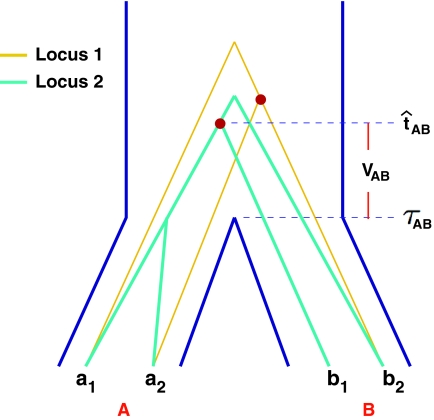If τ_AB is the true divergence time between taxa A and B, then the GLASS estimate of τ_AB is given by , i.e., the shortest time to an interspecific coalescence at some locus (Fig. 1).

FIG. 1.

The GLASS estimate of the divergence time between two taxa, A and B. Lineages a₁, a₂, b₁, and b₂ are sampled from taxa A and B, respectively, and gene trees for these lineages are shown at two loci, Locus 1 and Locus 2. Note that the individuals sampled need not be the same for all loci. The most recent interspecific coalescence at each locus is marked with a red dot. The GLASS estimate is the minimum interspecific coalescence time across loci. V_AB is the difference between the GLASS estimate and the divergence time.

The GLASS estimate of the species tree S is then constructed by applying single-linkage clustering to the set of estimates , where is the taxon set of the species tree. Specifically, the GLASS estimate of the distance between two sets of taxa C and C′ is defined by . The single-linkage clustering procedure involves grouping the two taxon sets with shortest distance, recomputing the distances among groups, and repeating the process until a single cluster remains.

The quantity is a consistent estimator of the pairwise divergence time τ_AB, because for any , the probability is positive that at locus ℓ, will exceed the divergence time by no more than ε time units. Thus, as more loci are sampled, it becomes increasingly likely that an interspecific coalescence at some locus will occur within ε time units of the divergence time τ_AB. The GLASS estimator is a consistent estimator of the species tree topology, because single-linkage clustering constructs a tree with the correct topology whenever is close enough to τ_AB for all A, .

Although the GLASS method is a consistent estimator of pairwise divergence times under the multispecies coalescent, the GLASS estimator systematically overestimates the divergence time τ_AB because interspecific coalescences occur more anciently than the divergence time under the model. It is well known that, at a given locus, the time of the first interspecific coalescence between a pair of taxa can greatly exceed the actual divergence time (Edwards and Beerli, 2000; Rosenberg and Feldman, 2002). Thus, especially when divergence times are small, the bias in GLASS estimates of divergence times can be large relative to the true times, leading to biased estimates of species tree branch lengths.

Here, by deriving the expected waiting time until the first interspecific coalescence occurs among L independent loci for a pair of taxa, we develop a correction to the GLASS estimator . We show that the corrected method, which we call iGLASS for “improved GLASS,” remains consistent for estimating pairwise divergence times in a species tree when incomplete lineage sorting is taken to be the sole source of gene tree discordance. We also show that each member in a particular class of clustering methods can be combined with pairwise iGLASS estimates to produce a statistically consistent estimator of the species tree topology. Through simulations, we demonstrate that in comparison with the GLASS estimator, the iGLASS estimator greatly reduces the bias and mean squared error (MSE) in pairwise estimates of species divergence times.

2. Correcting the Glass Method

To reduce the bias in the GLASS method's estimates of pairwise divergence times under the multispecies coalescent model, we assume that lineages evolve according to the model, and we derive the expectation of the difference between the GLASS estimator and the true divergence time. We then obtain a correction to the GLASS method by subtracting the expected difference from the GLASS estimate .

Under the multispecies coalescent model (Degnan and Rosenberg, 2009), in each branch of the species tree, the waiting time until i lineages coalesce to i − 1 lineages is exponentially distributed with mean coalescent time units of N generations, where N is the haploid effective size of the population in the branch. All of the pairs of lineages are equally likely to coalesce. When two populations merge backwards in time, all lineages remaining in the two daughter populations enter the ancestral population, and the coalescent process resumes in that branch.

To derive the distribution of the difference V_AB, we model the history of each pair of species A and B using two populations with constant haploid sizes N_A and N_B. These populations merge into an ancestral population of constant size N at the divergence time τ_AB (Fig. 1). For simplicity, throughout this article, all times are given in units of N generations. Furthermore, although we keep our derivations general by allowing N_A and N_B to take on arbitrary values, when we consider species trees with more than two taxa, we assume that the effective population sizes are equal in every branch of the species tree, and that the species tree is binary.

At time 0, corresponding to the present, and lineages are sampled at locus from taxa A and B, respectively. The quantities , and are assumed to be known. We also assume that the gene trees of sampled loci have been accurately estimated. Thus, the GLASS estimate is exactly equal to the time of the first interspecific coalescence between taxa A and B at some sampled locus.

We assume that for each pair of taxa A and B in the species tree, each taxon in the pair has the same distance τ_AB (in units of N generations) from the common ancestor of A and B. This assumption implies that when times are expressed in units of N generations, the species tree that we are inferring is ultrametric. In other words, for any three taxa X, Y, and Z, two of the distances , , and are equal and are greater than or equal to the remaining distance (Semple and Steel, 2003). Ultrametricity follows from the fact that one taxon in the triplet {X, Y, Z} is an outgroup to the other two, and we have assumed that the remaining two taxa are equidistant from it. Ultrametricity is required for the shared divergence time between a pair of taxa to be well-defined, and it also will be important for determining which clustering methods can be combined with iGLASS estimates of pairwise divergence times to produce consistent estimators of the species tree topology.

Let denote a particular value of the GLASS estimate computed from data and let denote the GLASS estimator, a random variable. To correct the observed GLASS estimate , we find the divergence time for which the expectation of the GLASS estimator under the multispecies coalescent model is equal to the observed value . Specifically, we solve

(1)

for τ_AB, and we take the solution as our estimate of the divergence time.

When the GLASS estimate is smaller than its smallest possible expected value , it is not meaningful to solve Equation (1). Therefore, we define the iGLASS estimate to be zero whenever . Defining the function , our estimator of the divergence time τ_AB, which we call the iGLASS estimator, is given by

(2)

Because is a polynomial in e^−τ_AB, as we will see, Equation (1) is transcendental and must be solved numerically. We now derive the quantity .

3. The Expected Minimal Interspecific Coalescence Time

Suppose that at locus , n_Aℓ and n_Bℓ lineages are sampled at time 0 from taxa A and B, respectively. Let and be random variables describing the numbers of lineages from taxa A and B remaining at the divergence time τ_AB at locus , and define the random vectors and . The expectation can be expressed as , where is the random difference between the GLASS estimator and the true divergence time. We now derive the expectation of V_AB.

Let denote the expectation of V_AB conditional on the event that K_A = k_A and K_B = k_B. Then

(3)

where h_n,k(τ; N_j) is the well-known probability that n lineages coalesce down to k lineages in time τ units of N generations in a population of constant size N_j (Tavaré, 1984). The distribution h_n,k(τ; N_j) is given by

(4)

where and , and where the factor N/N_j comes from the fact that time is expressed in units of N generations.

The expectation in Equation (3) was derived in the case of a single locus by Takahata (1989) using a recursive approach. A different recursive approach, which we present in Appendix A, can be used to compute in the case of multiple loci. The desired expectation is given by

(5)

in units of N generations, where e_ℓ is the ℓth standard basis vector of .

In addition to the mean, it is also of interest to obtain the distribution of the “overshoot” V_AB. Because both the unconditional probability distribution function and the conditional expectation can be obtained from the conditional distribution , we begin by computing . We first consider the case of a single locus, and we then extend the calculation to multiple loci.

3.1. Derivation of for one locus.

Consider a single locus and let k_A and k_B denote the numbers of lineages from taxa A and B remaining at the divergence time τ_AB. The quantity is then the distribution of the time to the first interspecific coalescence at the locus, measuring from time τ_AB.

To derive , recall that the time T_i until i lineages coalesce to i − 1 lineages is exponentially distributed with mean Thus, if k = k_A + k_B lineages remain at the divergence time, and if the first interspecific coalescence occurs on the Mth coalescence past the divergence time, then the waiting time V_AB until this coalescence can be expressed as the summation .

The location M in the sequence of coalescences of the first interspecific coalescence is itself a random variable and hence, V_AB has a Coxian distribution (Ross, 2007) with probability density function given by

(6)

In Equation (6), , where is the parameter of the ith waiting time T_k−(i−1). For m = 1, we define c_i,m to be unity.

The distribution in Equation (6) was derived by Takahata (1989). In Takahata's result, the probability Pr(M = m) is obtained recursively; however, it is possible to derive a closed-form solution. Rosenberg (2003) derived a closed-form expression that is equivalent to the cumulative distribution function of M. In Appendix B, we derive the closed-form of the probability mass function of M from Equation A8 of Rosenberg (2003). We obtain

(7)

whenever m ≤ k_A + k_B − 1, where , and where, as in Rosenberg (2003), is the number of ways in which k lineages can coalesce down to m lineages. Plugging expression (7) into (6) gives the formula for the distribution of V_AB in the case of one locus.

3.2. Derivation of for L loci.

We now extend formula (6) to multiple loci. Let be the random variable describing the time to the first interspecific coalescence at locus . We assume that all loci are independent, conditional on the species tree and its parameter values. Therefore, the cumulative distribution function of the minimum interspecific coalescence time is given by

(8)

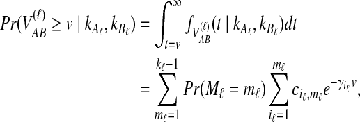
Here, is given by integrating Equation (6):

(9)

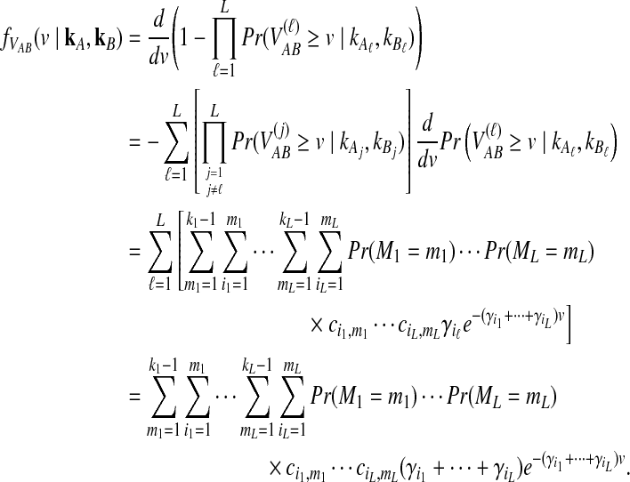
where k_ℓ = k_Aℓ + k_Bℓ is the total number of lineages remaining at the divergence time at locus ℓ. Plugging (9) into (8) and differentiating gives the density function :

(10)

In the last equality, we have brought the outer summation inside.

3.3. Closed-form expressions for and .

Closed-form expressions for and can now be computed using Equation (10). The unconditional density is given by

(11)

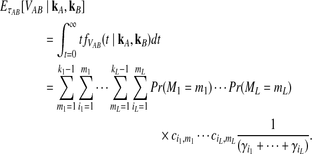
where the summation at a given locus in a given taxon (A or B) ranges from 1 to the number of sampled lineages at that locus in that taxon. The conditional expected value of V_AB for a collection of L loci is obtained by integrating Equation (10). This gives

(12)

The unconditional expected value can be computed by plugging either Equation (12) or the recursive Equation (5) into Equation (3), thereby completing the derivation of .

Thus, to obtain the iGLASS estimate from the GLASS estimate , we evaluate Equation (2), where

(13)

and where is given by either Equation (12) or Equation (5). The product is a polynomial in and thus, the inverse must be evaluated numerically. The iGLASS estimate of the species tree is then constructed by applying an appropriately chosen clustering method to the distance matrix of pairwise iGLASS time estimates. We discuss the choice of clustering method in Section 7.

4. An Approximation

The expectation (3) is expensive to compute either when the exact formula (Equation 12) is used or when the recursion (Equation 5) is used, due to the need to sum over all possible values of and . For this reason, we introduce a deterministic approximation that amounts to an assumption that, with probability one, the number of lineages remaining at the divergence time after coalescence along a species tree branch is the number expected at that time under the coalescent model. Thus, in our approximation, Equation (3) simplifies to

(14)

Using the approximation (14) eliminates the need to sum over all possible values of and , significantly reducing the computational cost.

However, we cannot implement this approximation using our current formulas because our expression for , Equation (12), requires k_A and k_B to be vectors of integers, whereas and need not be integers. Although it is an option to round each expected value, and , to the nearest integer, the approximation that results is somewhat imprecise. Thus, we take a different approach and re-derive an approximation to Equation (12) in such a way that it depends continuously on the number of lineages remaining at the divergence time.

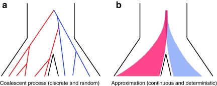
Our approach is to treat the number of lineages as a continuous quantity. We make use of a result from Maruvka et al. (2011), who demonstrated that if the initial number of lineages is large, the number of lineages remaining at time t behaves almost deterministically and is well approximated by simple deterministic functions that approximate the expected number of lineages at time t. We wish to be as accurate as possible, however, and we therefore approximate the number of lineages at time t by the expected number of lineages at that time (Fig. 2), rather than by an approximation to the expectation.

FIG. 2.

Approximation to the coalescent process in a pair of populations. (a) A random genealogy under the standard coalescent process. (b) An approximation to the coalescent process in which the number of lineages at time t is the expected number of lineages. Although the number of lineages remaining from a given taxon is deterministic in our approximation, the number of interspecific coalescences that occur in some time interval Δt is random, and it depends on the approximate numbers of lineages in the two taxa.

Define to be the expected number of lineages at time t units of N generations, given that n lineages exist at time t = 0. The expected number of lineages in a population of size N_j can be computed using Equation (4), or by the following formula from Tavaré (1984):

(15)

Formula (15) applies as long as the number of lineages at time t = 0 is an integer. However, as it is our goal to treat lineages as a continuous quantity, we would like to allow n to be any number greater than or equal to one.

When n is not a integer, we can introduce an “offset” ρ such that . Then for any n ≥ 1, we define the expected number of lineages at time t to be

(16)

where ρ is found by numerically solving using Equation (15). Thus, is a generalization of the expected number of lineages at time t to the case in which n is not integer-valued, and it allows us to treat the number of lineages as a continuous quantity. As we will see, the approximate expectation (14) computed using the approximation (16) is quite accurate even when only one or two lineages are sampled in the population.

We now use the quantity to derive an approximation for that depends continuously on k_A and k_B. We first derive an approximation to the conditional density in the case of a single locus, and we then generalize to many loci.

4.1. An approximation to for one locus.

As before, consider two taxa A and B. Let k_A and k_B be the numbers of lineages, not necessarily integers, that enter the ancestral population at the divergence time from taxa A and B, respectively. For the remainder of this derivation, it will simplify the notation if we measure time from a reference point at the divergence time τ_AB, rather than from the present. Thus, we take and to be the numbers of lineages remaining at time t from taxa A and B, counting from the divergence time.

Although and are deterministic quantities representing the expected numbers of lineages from taxa A and B, we continue to assume that the interactions between lineages are random. We assume that, in a small time interval [t, t + Δt], a coalescent event occurs with rate , given that no interspecific coalescence has occurred by time t. In addition, given that a coalescent event occurs in the interval [t, t + Δt], we approximate the probability that it is interspecific by , the conditional probability that a coalescence at time t involves one lineage from taxon A and one lineage from taxon B if the numbers of lineages are integer-valued. Thus, letting be the event that an interspecific coalescence occurs in the interval [a, b], letting be the event that an interspecific coalescence does not occur in the interval [a, b], and letting be the event that a coalescence of any kind occurs in the interval [a, b], we find that

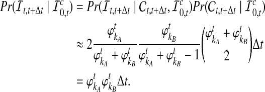Hence, the approximate probability that an interspecific coalescence does not occur in the interval [t, t + Δt], given that none has occurred more recently than time t, is

The probability that no interspecific coalescence occurs in the interval [0, t] can be approximated by the probability that no interspecific coalescence occurs in any of J small intervals of length Δt = t/J:

Thus, as J → ∞ we have Δt → 0, and

(17)

We now generalize this result to the case of many loci.

4.2. An approximation to for L loci.

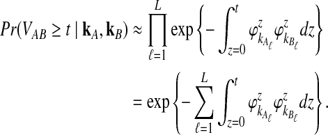
Let and be the deterministic approximations to the numbers of lineages remaining at time t from taxa A and B at locus ℓ. Then the probability that no interspecific coalescence occurs in any one of L independent loci in the interval [0, t] is approximately

(18)

4.3. The approximate iGLASS correction.

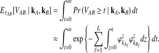
To get the expected time to the first interspecific coalescence at some locus, the approximation to Equation (12), we integrate:

(19)

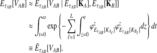
If we assume that the number of lineages remaining at the divergence time is the expected number of lineages at this time, then the approximate iGLASS correction, the approximation to Equation (3), is obtained by making the substitutions and into Equation (19):

(20)

This approximate expression is much faster to evaluate than Equation (3) because it does not require a sum over all possible values of and .

Because the values obtained from the approximation (Equation 20) differ from those obtained from the exact solution (Equation 3), we modify our definition of the iGLASS estimator (Equation 2) accordingly. We now define the function , and we define the approximate iGLASS estimator to be

(21)

As before, the approximate iGLASS estimate of the species tree is then constructed by applying any suitable clustering method to the pairwise approximate iGLASS estimates.

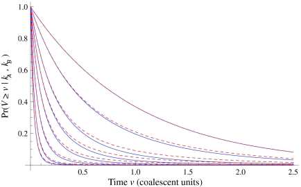
Although Equation (20) is an approximation, it can produce values that are remarkably close to the exact expectations. Figure 3 shows the exact survival function Pr(V_AB ≥ v) of V_AB (Equation 9) and the approximate survival function (Equation 18) for the case of one locus. From Figure 3, it can be seen that the approximation is exact when one lineage is sampled per taxon, because the expected number of lineages used in the approximation is always equal to one, the true number of lineages.

FIG. 3.

Approximate survival function (Equation 18) (red, dashed) and exact survival function (Equation 9) (blue) of the quantity for one locus, conditional on the numbers of lineages k_A and k_B remaining at the divergence time from each taxon. Pr(V ≥ v|K_A = k_A, K_B = k_B) is the probability that the GLASS estimate exceeds the divergence time τ_AB by more than v coalescent units. In order from top to bottom, the numbers of lineages that were used to generate the curves are (k_A, k_B) = (1,1), (1,2), (2,2), (2,3), (3,3), (3,5), (5,5), (5,7), where k_A is the number of lineages remaining in taxon A at the divergence time and k_B is the corresponding number of lineages remaining in taxon B. For the top curve, one lineage is sampled from each taxon and the approximation is exact.

For larger numbers of sampled lineages, as the time v is increased the approximation becomes slightly worse and then improves again. This result is a consequence of the behavior of the variability in the number of lineages over time. For small v, with very high probability the number of lineages is close to the number that were initially sampled, and the variance in the number of lineages is small. For intermediate v, greater variation exists in the number of lineages, and the approximation of the stochastic process of coalescence as a deterministic process is less appropriate. Finally, for large v, the number of lineages is equal to one with high probability, and the variance is again small. Thus, the expectation is a better approximation to the number of lineages for small and large v.

In practice, the approximate iGLASS correction (Equation 20) differs only slightly from the exact iGLASS correction, except in the case of a single locus (Fig. 4). Therefore, in our implementation of the iGLASS correction, we use the approximation (Equation 20), except in the case of a single locus, for which it is fast to compute the exact correction.

FIG. 4.

The difference between the approximate iGLASS correction (Equation 19) and the exact iGLASS correction (Equation 3). Each pixel in the heatmap shows the difference for a given divergence time τ_AB, a given number of lineages sampled per taxon, and a given number of loci. Within each block corresponding to a number of loci, the numbers of lineages sampled from each taxon at each locus are, from left to right, (n_A, n_B) = (1,1), (1,2), (1,3), (1,4), (2,2), (2,3), (2,4), (3,3), (3,4), and (4,4), where n_A is the number of lineages sampled from taxon A and n_B is the number sampled from taxon B.

5. Computational Complexity Of Approximate iGLASS

The computational complexity of the approximate iGLASS method is derived in Appendix C and is given by operations, where n is the maximal number of lineages sampled from any taxon at any locus, L is the number of loci, is the number of taxa, and Q is a tuning parameter that affects the accuracy of the numerical computations (see Appendix C). For fixed Q, the estimation procedure requires at most operations. In comparison, the GLASS method requires operations. Thus, in each parameter, the approximate iGLASS correction has computational complexity no greater than that of GLASS for a given precision Q.

6. Consistency of Exact and Approximate iGLASS

In this section, we show that both the exact and approximate iGLASS estimators (2) and (21) are consistent estimators of pairwise divergence times. We then show that applying any suitable clustering method to either exact or approximate iGLASS estimates of pairwise times produces a consistent estimator of the species tree topology. A family of clustering methods that gives rise to consistent estimation procedures is discussed in Section 7.

6.1. Exact and approximate iGLASS are consistent estimators of pairwise divergence times.

As we show in Theorem (D.1) in Appendix D, the GLASS method is a consistent estimator of pairwise divergence times. The exact and approximate iGLASS estimators (Equations 2 and 21) approach the GLASS estimator asymptotically in such a way that they are also consistent. We now prove this result.

Theorem 6.1

Given two taxa, A and B, the exact iGLASS method (Equation 2) is a consistent estimator of the divergence time τ_AB as the number of loci L → ∞.

Proof

Let τ_AB be the true divergence time, and let be the iGLASS correction to the GLASS method. We wish to show that converges in probability to τ_AB as the number of loci L → ∞. It is shown in Theorem D.1 that in probability as L → ∞. Thus, since convergence in distribution to a constant is equivalent to convergence in probability (Casella and Berger, 2002), it follows that in distribution as L → ∞. By Corollary E.3 in Appendix E, we have that C_AB ≤1/L → 0 as L → ∞. Thus, by Slutsky's theorem (Casella and Berger, 2002), in distribution (and in probability) as L → ∞.   ▪

A similar result holds for the approximate iGLASS method.

Theorem 6.2

Given two taxa, A and B, the approximate iGLASS method (Equation 21) is a consistent estimator of the divergence time τ_AB as the number of loci L → ∞.

Proof

In Lemma E.3 we show that the approximate iGLASS correction to the GLASS estimate also satisfies . The rest of the proof is the same as that of Theorem 6.1.   ▪

6.2. Exact and approximate iGLASS are consistent estimators of the species tree topology.

We now show that both the exact and approximate iGLASS methods are consistent estimators of the species tree topology whenever the clustering procedure applied to the estimates of pairwise divergence times has certain desirable properties. Let be a distance matrix whose elements are pairwise distances between taxa in the species tree S computed according to some distance measure. Let be an estimate of . Let ∥A∥_∞ denote the magnitude of the largest element in a matrix A. Following Atteson (1999), we give the following definition.

Definition 6.3

Let e(S) denote the length of the shortest edge in a binary species tree S. Let be the true matrix of pairwise distances between taxa in the tree S and let be an estimate of . Consider a clustering method that takes a distance matrix as input and returns a tree as output. The L_∞-radius ℓ_∞ of is the supremum over all quantities δ such that, for all species trees S and all estimates , is guaranteed to return the true topology whenever .

In other words, clustering methods with nonzero L_∞-radius construct a tree with the correct topology whenever the estimated distances are close to their true values.

In our case, we are working with pairwise estimates of divergence times rather than with pairwise distances. For an ultrametric tree, the divergence time between two taxa A and B is linearly related to the distance between the taxa and is equal to half the distance in the time units in which the tree is ultrametric: in this case coalescent units, generations, or years. Thus, when the species tree S is ultrametric, the L_∞-radius of a clustering method can be defined using divergence times instead of distances, as the supremum over all quantities δ such that returns a tree with the correct topology whenever .

We now prove that any clustering method with nonzero L_∞-radius, when combined with a consistent estimator of pairwise divergence times, produces a consistent estimator of the species tree topology. This result was assumed by Liu et al. (2010) in their proof that GLASS is consistent. The proof is straightforward; we include it for completeness.

Proposition 6.4

Consider a species tree S and let be a clustering method with nonzero L_∞-radius ℓ_∞. Let be an estimator of pairwise divergence time that is consistent as L → ∞. Then the estimator of the species tree S produced by applying clustering method to the collection of divergence time estimates obtained from is consistent for the tree topology as L → ∞.

Proof

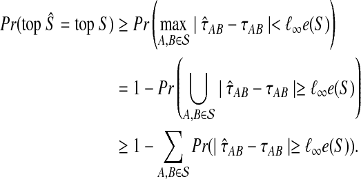
Let top S denote the topology of tree S. We wish to show that We have

(22)

In the first inequality, we have used the fact that the topology of S is correctly reconstructed whenever . Since is a probability, we have . Since is consistent, we have Thus, by the “squeeze theorem,” proving the result.   ▪

It follows from results (6.1), (6.2), and (6.4) that the exact and approximate iGLASS estimators generate consistent estimators of the species tree topology when combined with any clustering method that has nonzero L_∞-radius.

7. Clustering Methods with Nonzero L_∞-Radius

Gascuel and McKenzie (2004) showed that any agglomerative algorithm defined by the following procedure (excerpted from that article) has nonzero L_∞-radius, as long as the true species tree is ultrametric:

1. Input a set of estimates of pairwise distances .

2. Choose the pair of taxa or clusters X and Y that minimize , and combine them into a new cluster U.

3. For each cluster C ≠ X, Y, update the set of distances between C and the newly-formed cluster U according to , where . Leave all other distances unchanged.

4. Repeat (2) and (3) until one cluster remains.

Gascuel and McKenzie (2004) reported that the class of clustering methods that follow this procedure includes single-linkage clustering (Sneath, 1957), complete-linkage clustering (Sørensen, 1948), UPGMA (Sokal and Michener, 1958), and WPGMA (Sokal and Michener, 1958). These methods differ in the choice of λ_UC, which is allowed to depend on U and C. For instance, Gascuel and McKenzie (2004) noted that for single-linkage clustering, λ_UC = 1 when and λ_UC = 0 when (note that it is arbitrary which inequality is strict); for UPGMA, λ_UC = |X|/(|X| + |Y|), where |X| is the number of taxa in cluster X.

Atteson (1999) showed that the neighbor-joining method of Saitou and Nei (1987), which does not strictly follow the procedure of Gascuel and McKenzie (2004), also has nonzero L_∞-radius even when the true species tree is not ultrametric. Therefore, because we have assumed that the true species tree is ultrametric, by Proposition (6.4) we can combine neighbor-joining, or any method satisfying steps 1-4 above, with the iGLASS estimates of pairwise divergence times to produce a consistent estimator of the species tree topology.

8. A Version of the iGLASS Estimator Of Pairwise Divergence Times That is Unbiased When One Lineage is Sampled Per Taxon

Recall that in Equation (2), we forced the iGLASS estimates to be nonnegative. We will show that relaxing this requirement yields an unbiased estimator of pairwise divergence times in the case in which one lineage is sampled from each taxon.

Theorem 8.1

Consider two taxa A and B. If a single lineage is sampled from each taxon at each locus ℓ , then the estimator defined by for all is an unbiased estimator of the divergence time τ_AB.

Proof

Let and be the numbers of lineages remaining at locus ℓ from taxa A and B at the divergence time. When one lineage is sampled from each taxon at each locus, and equal one for all . Therefore, letting 1 be the vector of length L with all entries equal to 1, Equation (5) gives E[V_AB|K_A = 1, K_B = 1] = 1/L, and Equation (3) simplifies to . The function g(τ_AB) is then given by g(τ_AB) = τ_AB + 1/L, and its inverse by . Hence, g⁻¹(t) is defined for all and it is linear. Thus, by the linearity of the expectation operator,    ▪

This result implies that the iGLASS estimator defined by Equation (2) is also unbiased for most values of τ_AB whenever one lineage is sampled per taxon. Specifically, as we have assumed that gene trees are inferred with certainty, the GLASS estimate always exceeds the true divergence time τ_AB. Therefore, when one lineage is sampled per taxon at each locus and the true divergence time is greater than or equal to 1/L, it follows that and the iGLASS estimator is defined by . Thus, by Theorem 8.1, the iGLASS estimator will be unbiased in this case.

Note that when more than one lineage is sampled from either taxon, the probability in Equation (3) contains terms of the form , and thus, the quantity is no longer linear in τ_AB. In this case, is not linear in and therefore, we cannot use the relationship when more than one lineage is sampled per taxon. However, as we will see from simulations, the bias is still very small.

9. Comparison of Methods

We used simulations to compare the performance of iGLASS to that of GLASS, evaluating each method on the basis of bias and mean squared error (MSE). We first evaluated the methods for estimating pairwise divergence times, and we then applied them to larger trees.

9.1. Simulations

We simulated gene trees under the multispecies coalescent model for various species trees S, for various numbers of loci, and for various numbers of lineages sampled per taxon. In all simulations, all population sizes were equal to the same value N across the branches of the species tree.

To simulate a gene tree from a given species tree, we used a method similar to that of Rosenberg and Feldman (2002). Let branch i refer to the branch above node i in the species tree. Let t_i be the time at node i, and let be the time at the node ancestral to node i. Here, we extend our numbering to external branches, with t_i = 0 when i corresponds to a leaf node.

Let n_i be the number of lineages entering branch i at time t_i. If branch i is internal, then n_i is the sum of the numbers of lineages entering from its left and right daughter branches. If branch i is external, then n_i is equal to the number of lineages sampled from the corresponding taxon.

In each branch i, with the enumeration beginning with the external branches and proceeding towards the root in such a way that daughter branches have lower numbers than their parental branches, we first sampled the waiting time T_ni until the first coalescence from an exponential distribution with mean . If the sampled time T_ni exceeded , then we let the set of lineages exiting branch i equal the set that entered. Otherwise, we chose two lineages at random without replacement and allowed them to coalesce. We continued in this way, at each coalescence sampling the time to the next coalescence from an exponential distribution with mean , where q was the number of lineages remaining after the previous coalescence, until the sum of waiting times in the branch exceeded . The set of lineages remaining after the last coalescence to occur within branch i was then merged into the set of lineages entering its ancestral branch, along with the set of lineages entering from its sister branch, and the process was repeated in the ancestral branch. Simulations were run until all lineages coalesced to a single lineage. For trees with more than two taxa, the simulations were carried out using the software program ms (Hudson, 2002).

Let denote the number of lineages sampled from taxon X at locus ℓ . For a given species tree S together with a set of parameters consisting of a number of loci L and numbers of lineages , we first sampled r independent sets of L gene trees . For each set , we computed the GLASS estimate for all pairs of species using the GLASS algorithm (Section 1), without applying the single-linkage clustering step. From each observation , we then computed an observation of the exact iGLASS estimate, and an observation of the approximate iGLASS estimate. We thus obtained the sets of pairwise estimates , , and , for each set of gene trees . For species trees with more than two taxa, only and were computed.

For each set , we computed the GLASS estimate of the species tree by single-linkage clustering, and for each internal node i in this estimated species tree, we estimated the height of the node i by the distance between the two clusters combined on the step of the clustering method that produced the node. The clustering procedure was omitted for trees with two taxa because the estimates already provide estimates of the divergence time τ_AB. We then compared each estimated node height to its true value t_i, and we computed the average difference and the average squared difference .

Average bias in the GLASS method was estimated by , and average MSE by . The average bias and MSE in the exact and approximate iGLASS methods were estimated by the same procedure (using single-linkage clustering), but using the times and .

We denote the average bias and MSE in the exact iGLASS method by and , and we denote the average bias and MSE in the approximate iGLASS method by and .

9.2. Estimating pairwise divergence times.

To evaluate the performance of the three methods for estimating pairwise divergence times, we simulated gene trees under the multispecies coalescent from a species tree with two taxa, for various values of the parameters τ_AB, L, , and , and for r = 50,000 replicates. In varying the parameters and , we maintained the relationships and for all ℓ.

We considered values of 1, 5, 10, and 50 for L. However, because the exact iGLASS estimate is difficult to compute in the case of both multiple loci and large numbers of lineages, only the GLASS estimate and approximate iGLASS estimate were computed when both the number of loci and the number of lineages were large.

9.2.1. Bias

Figure 5 indicates that especially for small divergence times, the bias in the GLASS estimate can be large relative to the divergence time. Whenever a single lineage is sampled from each taxon, the bias in the GLASS method is 1/L in coalescent units of N generations, regardless of the divergence time. One lineage always remains at the divergence time from each taxon at each locus, and therefore, the expected time to the first interspecific coalescence is the expectation of the minimum of L independent exponentially distributed random variables, each with a mean of one coalescent time unit. For example, in a haploid population with an effective size of N = 10, 000, if the GLASS estimate is based on a single lineage sampled from each population at each of 20 loci, then the bias in the GLASS estimate is 10,000/20 = 500 generations.

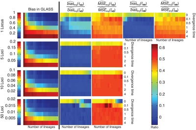
FIG. 5.

Comparison of bias and mean squared error for the GLASS, exact iGLASS, and approximate iGLASS methods for two taxa and one locus. All values were computed using 50,000 simulation replicates. In each of the fourteen small heatmap panels, the divergence time between two taxa A and B is given in coalescent units on the y-axis. In each heatmap, the divergence times are, from top to bottom, τ_AB = 0, 0.1, 0.5, 1, 2, and 4 coalescent units. In each heatmap, the numbers of lineages sampled from each taxon are given on the x-axis in the format (n_A, n_B), where n_A is the number of lineages sampled from taxon A, and n_B is the number sampled from taxon B. From left to right, the numbers of lineages in each column are (n_A, n_B) = (1,1), (1,3), (1,5), (1,10), (1,15), (1,20), (3,3), (3,5), (3,10), (3,15), (3,20), (5,5), (5,10), (5,15), (5,20), (10,10), (10,15), (10,20), (15,15), (15,20), (20,20).

Although sampling multiple lineages from each population can greatly reduce the bias for low divergence times, it does not reduce the bias for larger divergence times. As noted by Mossel and Roch (2010), when τ_AB is measured in units of generations, the probability that a single lineage remains at the top of the branch corresponding to taxon A is bounded below by and the probability that a single lineage remains at the top of the branch corresponding to taxon B is bounded below by (Tavaré, 1984). This bound can be made arbitrarily close to one by increasing the divergence time and, as the divergence time increases, the GLASS estimate approaches the value of the GLASS estimate when one lineage is sampled per taxon, or 1/L coalescent units.

To compare the estimated bias in the exact and approximate iGLASS methods to the estimated bias in the GLASS method, we computed the ratios and (Fig. 5). For most values of the divergence time, the bias in the approximate iGLASS method is negligible compared to the bias in the GLASS method; although it is considerably larger in magnitude for small values of τ_AB, the bias ratio continues to be less than 1. The bias is not entirely negligible in this case because we define the exact and approximate iGLASS estimates to be zero whenever the GLASS estimate is lower than its smallest possible expected time (Equations 2 and 21). Thus, when the GLASS estimate is small, instead of subtracting a positive quantity from the GLASS estimate to produce the iGLASS estimate, we estimate the divergence time to be zero, resulting in an iGLASS estimate (exact or approximate) that is biased upwards. This truncation prevents the iGLASS estimators from completely eliminating the bias, but it also leads to a decrease in variance, which ultimately leads to a lower mean squared error at these divergence times. The decrease in MSE due to lower variance can be seen by the yellow bars across the tops of the MSE graphs in Figure 5.

9.2.2. Mean squared error

The ratios and are shown in Figure 5 for various values of τ_AB, n_A, and n_B. From these plots, we can see that and are roughly 1/2, and that they appear to approach 1/2 as τ_AB increases.

To see why this is reasonable, consider the case in which a single lineage is sampled per taxon at each locus. In this case, the “overshoot” in the GLASS estimate, , is distributed exponentially with mean 1/L. Thus, the bias in the GLASS estimator is , its variance is Var(V_AB) = 1/L², and its MSE is . The variance in the GLASS estimator then accounts for half of the mean squared error when one lineage is sampled per taxon.

When one lineage is sampled per taxon, the iGLASS correction to the GLASS estimator is computed by subtracting a constant quantity 1/L from the GLASS estimate, except when is in the region , which decreases in size as L → ∞. Thus, the variance of the (exact or approximate) iGLASS estimator is nearly equal to the variance of the GLASS estimator. As Theorem 8.1 indicates, when a single lineage is sampled per taxon, the iGLASS estimator is almost unbiased. Thus, when a single lineage is sampled per taxon, the MSE in the (exact or approximate) iGLASS estimator is approximately equal to the variance in the GLASS estimator, which is half the MSE in the GLASS estimator. Because and approach one in probability as τ_AB → ∞, we expect that will approach as τ_AB increases to infinity.

9.3. Exact versus approximate iGLASS

In the majority of our simulations, we have used the approximate iGLASS correction rather than the exact method because the exact correction is difficult to compute. However, consider the panels in the first row of Figure 5 that correspond to the case of one locus. It can be seen that the bias and MSE in the approximate iGLASS method are very similar to the bias and MSE in the exact iGLASS method. This result indicates that making the approximation (Equation 20) has little effect on the performance of the iGLASS estimator in the case of one locus. Because Figure 4 indicates that the approximation is least accurate in the case of a single locus, the similarity of the bias and MSE for the exact and approximate methods in the case of one locus suggests that making the approximation generally has little effect on the performance of the iGLASS method relative to that of GLASS.

9.4. iGLASS for larger trees

Figure 6 shows the ratios and computed over r = 50,000 replicates for two different five-taxon species trees similar to those used by Liu et al. (2010) to evaluate the performance of the GLASS method. One internal branch of the tree is short enough that the most likely gene tree given the species tree does not have the topology of the true tree. In other words, the tree is in the anomaly zone of Degnan and Rosenberg (2006).

FIG. 6.

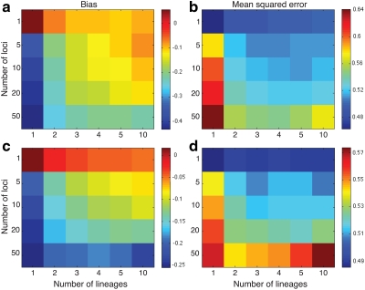
Comparison of mean squared error and bias in the approximate iGLASS and GLASS methods for two five-taxon species trees used in Liu et al. (2010) to evaluate the GLASS method. In Newick format, the tree in (a) and (b), a caterpillar, is given by ((((E:0.5, D:0.5):0.025, C:0.525):0.025, B:0.55):10.0, A:10.55). The tree in (c) and (d), another 5-taxon caterpillar, is ((((E:0.5, D:0.5):0.2, C:0.7):1, B:1.7):10.0, A:11.7). The first tree is in the anomaly zone; the second tree is not. All values were computed using 50,000 replicates. The clustering method applied to the approximate iGLASS estimates was single-linkage. (a) and (c): The ratio . (b) and (d): The ratio .

From Figure 6, we see that the average bias in the iGLASS estimate is often considerably less than that of the GLASS estimate. The improvement in the bias is best for small numbers of loci and decreases as the number of loci increases. However, the bias in the GLASS method itself decreases quickly as the number of loci is increased.

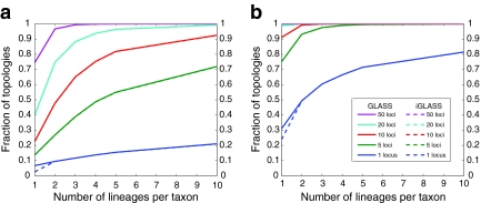
Note that although the iGLASS correction improves the bias and MSE in the estimates of species tree node heights, it does not improve the accuracy in estimating topologies. For both species trees ((((E:0.5, D:0.5):0.025, C:0.525):0.025, B:0.55):10.0, A:10.55) and ((((E:0.5, D:0.5):0.2, C:0.7):1, B:1.7):10.0, A:11.7) that we considered, the GLASS and iGLASS methods have identical accuracies for estimating the topology. However, for the case in which only one lineage is sampled at only one locus, the GLASS method has slightly higher accuracy for inferring the topology (Fig. 7).

FIG. 7.

The fraction of tree topologies correctly inferred by the approximate iGLASS and GLASS methods for two different five-taxon species trees. The tree in (a) is the same tree considered in Figure 6a,b. The tree in (b) is the same tree considered in Figure 6c,d. Plots show the fraction of 50,000 simulated data sets in which the species tree topology was correctly inferred by GLASS and approximate iGLASS.

The reduction in accuracy for the case of one lineage and one locus was due to the fact that in this case, the iGLASS method estimated more than one pairwise divergence time in the species tree to be zero, resulting in ties that were sometimes resolved to produce a clade that was not on the true species tree. Multiple estimates of zero were produced in this case because the smallest possible expected value of the GLASS estimate for a pair of taxa was equal to one, which was greater than at least two of the node heights in each tree that we considered (0.5 and 0.525 for the first tree, and 0.5 and 0.7 for the second tree).

For all other parameter values we considered, was smaller than all of the node heights in either tree, and no estimates of zero were produced. For example, when two lineages were sampled per taxon, the smallest possible expected GLASS estimate was E₀[T_AB] = 0.39, which is smaller than 0.5, the smallest node height in either tree. Similarly, when one lineage was sampled per taxon at 5 loci, the smallest expected interspecific coalescence time was E₀[T_AB] = 0.2. Consequently, for all cases we considered except for the case of one sampled lineage per taxon at one locus, the accuracy of the iGLASS method for estimating topologies was the same as that of the GLASS method.

10. Discussion

For two taxa, A and B, we have derived a closed-form expression for the distribution of , the waiting time to the first interspecific coalescence across L loci, measuring from the divergence time τ_AB. By computing the expectation E_τAB[V_AB], we constructed a correction to the GLASS estimator of pairwise divergence times, which we call the iGLASS estimator.

Maruvka et al. (2011) have demonstrated that simple functions of time t in a population of constant size can provide useful deterministic continuous approximations of the number of lineages remaining at time t under the standard coalescent model. By approximating the number of lineages at time t by , the expected number of lineages remaining at time t when x lineages are sampled at time t = 0 and when x is not necessarily an integer, we derived an approximation to the exact iGLASS estimator that is faster to compute than the exact value, and that is quite accurate even when the number of lineages is small.

Through simulations, we have shown that the exact and approximate iGLASS estimators reduce the bias in the GLASS estimates of pairwise divergence times. In addition, the exact iGLASS estimator and its approximation generally reduce the mean squared error in the GLASS estimate of pairwise divergence times by approximately one half. This reduction accords with a theoretical prediction in the case in which a single lineage is sampled per taxon.

In our simulations, the accuracy of the iGLASS method for estimating topologies was similar to that of the GLASS method. In the case in which one lineage was sampled per taxon at one locus, iGLASS was slightly poorer, due to the fact that iGLASS produces divergence time estimates of zero whenever the GLASS estimate is smaller than its smallest possible expected value, . Because is smaller when the number of sampled lineages or loci is larger, divergence time estimates of zero are less likely when more lineages or loci are sampled. Therefore, the accuracy of the topology estimates produced by iGLASS are likely to be the same as those produced by GLASS whenever sufficiently many lineages or loci are sampled.

We have shown that the exact iGLASS estimator and its approximation are consistent estimators of the pairwise divergence time between a pair of taxa. Further, we have proven that applying any clustering method with nonzero L_∞-radius to the pairwise iGLASS estimates produces a statistically consistent estimator of the species tree topology.

Assuming that gene trees have been correctly inferred, the bias in the GLASS method itself decreases to zero quickly as the number of loci increases. Thus, our correction produces the greatest improvement when information is available for relatively few loci. As we have seen, however, the approximate iGLASS correction is fast to compute even for large numbers of loci, requiring only operations for a given level of precision, compared to operations for GLASS. Consequently, our new estimator provides a method that is reasonable to implement even when information is available at many loci.

11. Appendix A

A recursive formula for

In Appendix A, we derive Equation (5), the expected value of the difference , conditional on the numbers of lineages that remain at each locus at the divergence time. Let C_ℓ be the event that the first coalescence occurs in locus . We then recursively consider what happens on the next coalescent event:

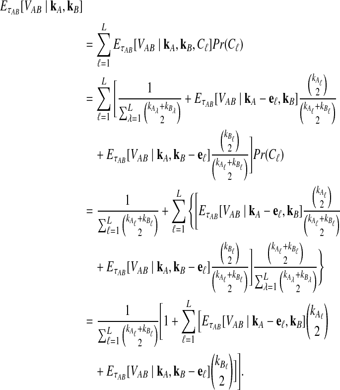Above, λ is a “dummy” summation variable. The second equality can be understood as follows. Because the time to the first coalescent event at locus ℓ is exponentially distributed with mean , the time to the first coalescence at some locus is distributed as the minimum of L such random variables. Therefore, the expected time to the first coalescent event is coalescent units. We must always wait this long on average before the first interspecific coalescent event. Given that the first coalescence occurs at locus ℓ, if the coalescence occurs among lineages from taxon A, an event that occurs with probability , we must wait on average an additional time units. Similarly, with probability , we must wait an additional time units on average. Finally, if the first coalescence at locus ℓ is interspecific, an event that has probability , no further waiting is necessary.

In the third equality, the term does not depend on ℓ and can be brought outside. Additionally, because the time to the first coalescence at locus ℓ is exponentially distributed with mean , the first coalescence occurs at locus ℓ with probability .

12. Appendix B

Derivation of Equation (7)

In Appendix B, we rely on results from Rosenberg (2003) to derive the probability distribution of M, the number of coalescent events up to and including the first interspecific coalescence, counting backwards in time from the divergence time.

Suppose that k_A and k_B lineages from taxa A and B, respectively, remain at time τ_AB. Equation (A8) of Rosenberg (2003) gives the probability that an interspecific coalescence occurs among these lineages on or before the (k − w)th coalescence, where k = k_A + k_B. This probability is

(B.1)

where I_n,k = [n!(n − 1)!]/[2^n−kk!(k − 1)!] (Rosenberg, 2003) is the number of ways in which n lineages can coalesce down to k lineages, and (Rosenberg, 2003) is the number of ways of “interweaving” the coalescent events among lineages only from taxon A with the coalescent events among lineages only from taxon B.

Each term in the summation (B.1) is the joint probability that the first interspecific coalescence occurs when the k_A and k_B lineages have x and y ancestors, respectively, and that the first interspecific coalescence occurs on or before the (k − w)th coalescence. If w = 1, then each term is just the probability that the first interspecific coalescence occurs when the k_A and k_B lineages have x and y ancestors.

Since different choices of x and y (say, (x₁, y₁) and (x₂, y₂) where x₁ ≠ x₂ or y₁ ≠ y₂, or both) correspond to mutually exclusive events, and since the sum x + y specifies M through the relationship x + y = k − M + 1, to derive the probability that the first interspecific coalescence is the Mth coalescence (Equation 7), we can set w = 1 and sum over all x and y such that x + y = k − M + 1, i.e., over all mutually exclusive events corresponding to the case in which the first interspecific coalescence is the Mth coalescence.

To determine the values of x and y corresponding to the case M = m, we can write x = k − m + 1 − y. Note that x is at most k_A and at least 1, and thus, 1 ≤ x ≤ min{k − m, k_A}. Similarly, by symmetry in x and y, 1 ≤ y ≤ min{k − m, k_B}, giving x = k − m + 1 − y ≥ k − m + 1 − min{k − m, k_B} = max{1, k_A − m + 1}. This inequality yields the constraint max{1, k_A − m + 1} ≤ x ≤ min{k − m, k_A}. Thus, we obtain

Making the change of variables η = k_A − x and noting that k_B − y = m − 1 − η because k_A + k_B − m + 1 = x + y, we get

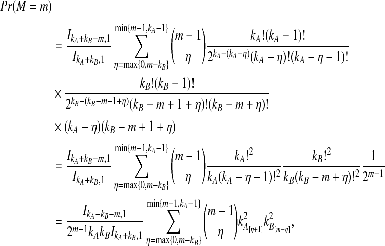
Using I_n,k = [n!(n − 1)!]/[2^n−kk!(k − 1)!] and , we get

(B.2)

where k_[i] = k!/(k − i)!.

When either k_A = 1 or k_B = 1, Equation (B.2) has a particularly simple form. Without loss of generality, suppose that k_B = 1. Then max{0, m − k_B} = m − 1 because m ≥ 1, and min{m − 1, k_A − 1} = m − 1 because m ≤ k_A + k_B − 1 = k_A. Therefore, using k = k_A + 1, Equation (B.2) simplifies as follows:

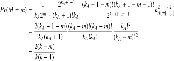(B.3)

13. Appendix C.

Computational complexity of approximate iGLASS

We now compute the computational complexity of the approximate iGLASS method, Equation (21). To compute the iGLASS correction for each pair of taxa X and Y in , we first evaluate Equation (20) for many different values of τ_XY. In particular, to numerically obtain the inverse in Equation (21), we compute Equation (20) for each divergence time estimate τ_XY in the set , where Δt is a fixed time-step and . We then estimate τ_XY by the value that minimizes the quantity .

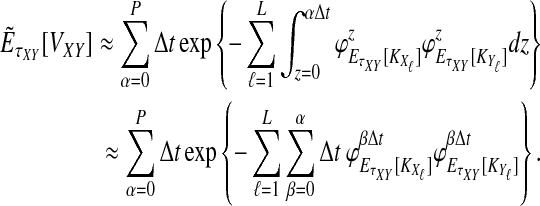
To evaluate the integral in Equation (20), we assume that numerical integration is carried out by computing the Riemann sum with fixed step-size Δt. We truncate the outer integral at PΔt, where P is large enough that the tail of the outer integral in Equation (20) is smaller than some predefined value ε > 0. For a given value of ε, a sufficiently-large value of P can be found by bounding the integral in Equation (20). The bound can be obtained by noting that for all n and z in , and thus, the integrand in Equation (20) is smaller than exp{ − Lt}, which is easily integrated. Converting the integrals in Equation (20) to summations gives

(C.1)

Once and have been pre-computed and stored for all values at which they are evaluated in the summation, the exponent in Equation (C.1) requires O(Lα) operations, where α is the index in the outermost summation. Thus, we have the following result:

After pre-computing the terms in the summand, the summation (C.1) requires O(LP²) operations.

For each taxon , let ; in other words, Γ_XΔt is, to precision Δt, the maximum pairwise divergence time between taxon X and any other taxon. For each and for each , we must ultimately compute for each , and we must compute for each and for each . However, note that , and note that by definition (Equations (15) and (16)). Therefore, we have for all , and thus, it suffices to pre-compute for all for each and for each .

Let be the maximal number of lineages sampled from any taxon, and let . Then for a given taxon and for a given , the amount of time needed to compute for all is bounded by the time needed to compute for all .

Because the summand in Equation (15) requires O(n) operations, (a rising factorial and a falling factorial totaling n multiplications), computing Equation (15) for a given value of t requires O(n²) operations. Therefore, evaluating (15) for each time t in requires O(n²Q) operations, and pre-computing for all also requires O(n²Q) operations. This gives the following result:

Pre-computing for all for all and for all ℓ requires operations.

Once all values of have been pre-computed and stored, Equation (C.1) must be computed for each for each pair of taxa . Equation (C.1) requires O(LP²) operations for each value of τ. Therefore, because Γ_XY ≤ Q, computing (C.1) for a pair of taxa requires O(LP²Q) operations. Because P ≤ Q, this simplifies to O(LQ³) operations. Therefore, computing (C.1) for all pairs of taxa requires operations. Combining this quantity with the number of operations necessary to pre-compute the values of gives the following result:

Including all pre-computations, the total number of operations required to compute Equation (C.1) for all pairs of taxa is .

Note that once all values of have been pre-computed and stored, the cost of computing (C.1) does not depend on the magnitude of the , only on the number of terms in the summation. Thus, the complexity only depends on n through the pre-computation step.

The only other computations needed to compute the approximate iGLASS correction are those associated with finding arg and those associated with the single-linkage clustering step. We must perform searches to find the value of τ that minimizes for each of the pairs of taxa. An exhaustive search is bounded by the number of values of τ, which is always less than or equal to Q. Thus, correcting the GLASS method requires operations. Finally, single-linkage clustering requires at most operations (Gordon, 1996). Thus, the entire correction procedure requires operations. Terms can be combined to get the following result:

The entire approximate iGLASS correction procedure requires operations.

It is useful to compare the complexity of approximate iGLASS to the complexity of GLASS for a given precision. The choices of Δt and P determine the precision in computing the approximate iGLASS correction, in other words, the error between the outcome of the numerical steps that we have just outlined, and the outcome of exactly computing Equation (20) and exactly solving Equation (21). Together, Δt and P determine . Thus, Q is a tuning parameter that affects the precision in our numerical steps. For fixed Q, the complexity of approximate iGLASS is . In comparison, a similar analysis demonstrates that the GLASS method requires operations.

14. Appendix D

Consistency of GLASS for divergence times

Mossel and Roch (2010) proved that the GLASS method is a consistent estimator of the species tree topology as the number of loci approaches infinity. Liu et al. (2010) proved that the GLASS estimator is consistent for pairwise divergence times in the case in which a single lineage is sampled per taxon.

Here, we prove that GLASS is a consistent estimator of pairwise divergence times in the case in which arbitrarily many lineages are sampled per taxon. Our argument is a minor extension of the consistency proof in Liu et al. (2010).

Theorem D.1

Consider two taxa, A and B, with divergence time τ_AB. The GLASS estimator is a consistent estimator of τ_AB.

Proof

At each locus ℓ , consider a lineage a_ℓ sampled at random from taxon A and a lineage b_ℓ sampled at random from taxon B. The time to the first interspecific coalescence at locus ℓ is less than or equal to the coalescence time between a_ℓ and b_ℓ, which we denote by . Therefore, using the fact that the GLASS estimate is given by , and following Liu et al. (2010), we obtain . Here, to obtain the last equality, we have used the fact that is exponentially distributed with mean 1 coalescent unit of N generations. Thus, we have

from which it follows that as L → ∞ by the “squeeze theorem.”   ▪

15. Appendix E

iGLASS and approximate iGLASS are consistent estimators of pairwise divergence times

Here, we prove that the expectation of the difference between the GLASS estimate and the divergence time τ_AB is bounded above by 1/L. Thus, as L → ∞. Using Equation (1), we then show that the difference between the GLASS estimator and the iGLASS estimator is bounded above by 1/L. Thus, the difference goes to 0 as L → ∞. A similar result is proven for the expectation used in the approximate iGLASS correction (Equation 21).

Since GLASS is a consistent estimator of pairwise divergence times, these results can be used to show that exact iGLASS and approximate iGLASS are consistent estimators of pairwise divergence times, as they converge to the same limit as the GLASS estimator in the limit L → ∞.

Lemma E.1

For taxa A and B, let be the expectation of the difference between the GLASS estimate and the divergence time τ_AB. Then .

Proof

In Theorem D.1, we saw that for all . Thus,

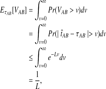proving the result.   ▪

Lemma E.2

The approximation satisfies .

Proof

For any n and t, the expected number of lineages remaining at any given time t is at least 1. Therefore, for any ℓ

Consequently,

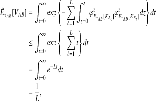proving the result.   ▪

The following corollary proves that after the correction procedure (Equation 2), both the exact and approximate iGLASS estimates differ from the GLASS estimate by at most 1/L coalescent units.

Corollary E.3

For two taxa A and B, let and be the differences between the GLASS estimate and the exact and approximate iGLASS estimates, respectively. Then C_AB ≤1/L and .

Proof

Using Equation (2), if , then the iGLASS estimate is obtained by solving for τ_AB. In this case, the difference C_AB is at most 1/L by Lemma E.1. On the other hand, if , then the iGLASS estimate is given by . Since [0, E₀[V_AB]) ⊆ [0, 1/L) by Lemma E.1, we have . Thus, in both cases, C_AB ≤ 1/L.

The same argument using Lemma E.2 and Equation (21) rather than Lemma E.1 and Equation (2) establishes , proving the result.   ▪

Acknowledgments

We are grateful to Michael DeGiorgio, Lucy Huang, and Laura Helmkamp for helpful discussions, and to Lucy Huang for suggesting the name iGLASS. We also thank two anonymous reviewers for their careful reading and helpful suggestions, and for simplifying the proofs of Theorem D.1 and Lemma E.1. This work was supported by the NSF (grants DEB-0716904 and DBI-1146722), by a grant from the Burroughs Wellcome Fund, and by the NIH (training grant T32 HG00040).

Disclosure Statement

No competing financial interests exist.

References

- Atteson K. The performance of neighbor-joining methods of phylogenetic reconstruction. Algorithmica. 1999;25:251–278. [Google Scholar]
- Casella G. Berger R.L. Statistical Inference. 2nd. Duxbury Press; Pacific Grove, CA: 2002. [Google Scholar]
- Degnan J.H. Rosenberg N.A. Discordance of species trees with their most likely gene trees. PLoS Genet. 2006;2:762–768. doi: 10.1371/journal.pgen.0020068. [DOI] [PMC free article] [PubMed] [Google Scholar]
- Degnan J.H. Rosenberg N.A. Gene tree discordance, phylogenetic inference, and the multispecies coalescent. Trends Ecol. Evol. 2009;24:332–340. doi: 10.1016/j.tree.2009.01.009. [DOI] [PubMed] [Google Scholar]
- Edwards S.V. Beerli P. Gene divergence, population divergence, and the variance in coalescence time in phylogeographic studies. Evolution. 2000;54:1839–1854. doi: 10.1111/j.0014-3820.2000.tb01231.x. [DOI] [PubMed] [Google Scholar]
- Edwards S.V. Liu L. Pearl D.K. High-resolution species trees without concatenation. Proc. Natl. Acad. Sci. USA. 2007;104:5936–5941. doi: 10.1073/pnas.0607004104. [DOI] [PMC free article] [PubMed] [Google Scholar]
- Ewing G.B. Ebersberger I. Schmidt H.A., et al. Rooted triple consensus and anomalous gene trees. BMC Evol. Biol. 2008;8:118. doi: 10.1186/1471-2148-8-118. [DOI] [PMC free article] [PubMed] [Google Scholar]
- Gascuel O. McKenzie A. Performance analysis of hierarchical clustering algorithms. J. Classif. 2004;21:3–18. [Google Scholar]
- Gordon A.D. Hierarchical clustering. In: Arabie P., editor; Hubert L.J., editor; Soete D., editor. Clustering and Classification. World Scientific Publishing Co; River Edge, NJ: 1996. pp. 65–121. [Google Scholar]
- Hudson R.R. Generating samples under a Wright-Fisher neutral model. Bioinformatics. 2002;18:337–338. doi: 10.1093/bioinformatics/18.2.337. [DOI] [PubMed] [Google Scholar]
- Kubatko L.S. Carstens B.C. Knowles L.L. STEM: species tree estimation using maximum likelihood for gene trees under coalescence. Bioinformatics. 2009;25:971–973. doi: 10.1093/bioinformatics/btp079. [DOI] [PubMed] [Google Scholar]
- Liu L. Yu L. Kubatko L., et al. Coalescent methods for estimating phylogenetic trees. Mol. Phylogenet. Evol. 2009a;53:320–328. doi: 10.1016/j.ympev.2009.05.033. [DOI] [PubMed] [Google Scholar]
- Liu L. Yu L. Pearl D.K., et al. Estimating species phylogenies using coalescence times among sequences. Syst. Biol. 2009b;58:468–477. doi: 10.1093/sysbio/syp031. [DOI] [PubMed] [Google Scholar]
- Liu L. Yu L. Pearl D.K. Maximum tree: a consistent estimator of the species tree. J. Math. Biol. 2010;60:95–106. doi: 10.1007/s00285-009-0260-0. [DOI] [PubMed] [Google Scholar]
- Maddison W.P. Gene trees in species trees. Syst. Biol. 1997;46:523–536. [Google Scholar]
- Maruvka Y.E. Shnerb N.M. Bar-Yam Y., et al. Recovering population parameters from a single gene genealogy: an unbiased estimator of the growth rate. Mol. Biol. Evol. 2011;28:1617–1631. doi: 10.1093/molbev/msq331. [DOI] [PubMed] [Google Scholar]
- Mossel E. Roch S. Incomplete lineage sorting: consistent phylogeny estimation from multiple loci. IEEE/ACM Trans. Comput. Biol. Bioinform. 2010;7:166–171. doi: 10.1109/TCBB.2008.66. [DOI] [PubMed] [Google Scholar]
- Nichols R. Gene trees and species trees are not the same. Trends Ecol. Evol. 2001;16:358–364. doi: 10.1016/s0169-5347(01)02203-0. [DOI] [PubMed] [Google Scholar]
- Rannala B. Yang Z. Bayes estimation of species divergence times and ancestral population sizes using DNA sequences from multiple loci. Genetics. 2003;164:1645–1656. doi: 10.1093/genetics/164.4.1645. [DOI] [PMC free article] [PubMed] [Google Scholar]
- Rannala B. Yang Z. Phylogenetic inference using whole genomes. Annu. Rev. Genomics Hum. Genet. 2008;9:217–231. doi: 10.1146/annurev.genom.9.081307.164407. [DOI] [PubMed] [Google Scholar]
- Rosenberg N.A. The shapes of neutral gene genealogies in two species: probabilities of monophyly, paraphyly, and polyphyly in a coalescent model. Evolution. 2003;57:1465–1477. doi: 10.1111/j.0014-3820.2003.tb00355.x. [DOI] [PubMed] [Google Scholar]
- Rosenberg N.A. Feldman M.W. The relationship between coalescence times and population divergence times. In: Slatkin M., editor; Veuille M., editor. Modern Developments in Theoretical Population Genetics. Oxford University Press; Oxford, UK: 2002. pp. 130–164. [Google Scholar]
- Ross S. Introduction to Probability Models. 9th. Academic Press; New York: 2007. [Google Scholar]
- Saitou N. Nei M. The neighbor-joining method: a new method for reconstructing phylogenetic trees. Mol. Biol. Evol. 1987;4:406–425. doi: 10.1093/oxfordjournals.molbev.a040454. [DOI] [PubMed] [Google Scholar]
- Semple C. Steel M. Phylogenetics. Oxford University Press; New York: 2003. [Google Scholar]
- Sneath P.H.A. The application of computers to taxonomy. J. Gen. Microbiol. 1957;17:201–226. doi: 10.1099/00221287-17-1-201. [DOI] [PubMed] [Google Scholar]
- Sokal R. Michener C. A statistical method for evaluating systematic relationships. Univ. Kans. Sci. Bull. 1958;38:1409–1438. [Google Scholar]
- Sørensen T. A method of establishing groups of equal amplitude in plant sociology based on similarity of species content and its application to analyses of the vegetation on Danish commons. K. Dan. Vidensk. Selskab Biol. Skrift. 1948;5:1–34. [Google Scholar]
- Takahata N. Gene genealogy in three related populations: consistency probability between gene and population trees. Genetics. 1989;122:957–966. doi: 10.1093/genetics/122.4.957. [DOI] [PMC free article] [PubMed] [Google Scholar]
- Tavaré S. Line-of-descent and genealogical processes, and their applications in population genetics models. Theor. Popul. Biol. 1984;26:119–164. doi: 10.1016/0040-5809(84)90027-3. [DOI] [PubMed] [Google Scholar]
- Than C. Nakhleh L. Species tree inference by minimizing deep coalescences. PLoS Comput. Biol. 2009;5:e1000501. doi: 10.1371/journal.pcbi.1000501. [DOI] [PMC free article] [PubMed] [Google Scholar]