Improvement of Tablet Coating Uniformity Using a Quality by Design Approach

Abstract

A combination of analytical and statistical methods is used to improve a tablet coating process guided by quality by design (QbD) principles. A solid dosage form product was found to intermittently exhibit bad taste. A suspected cause was the variability in coating thickness which could lead to the subject tasting the active ingredient in some tablets. A number of samples were analyzed using a laser-induced breakdown spectroscopy (LIBS)-based analytical method, and it was found that the main variability component was the tablet-to-tablet variability within a lot. Hence, it was inferred that the coating process (performed in a perforated rotating pan) required optimization. A set of designed experiments along with response surface modeling and kriging method were used to arrive at an optimal set of operating conditions. Effects of the amount of coating imparted, spray rate, pan rotation speed, and spray temperature were characterized. The results were quantified in terms of the relative standard deviation of tablet-averaged LIBS score and a coating variability index which was the ratio of the standard deviation of the tablet-averaged LIBS score and the weight gain of the tablets. The data-driven models developed based on the designed experiments predicted that the minimum value of this index would be obtained for a 6% weight gain for a pan operating at the highest speed at the maximum fill level while using the lowest spraying rate and temperature from the chosen parametric space. This systematic application of the QbD-based method resulted in an enhanced process understanding and reducing the coating variability by more than half.

INTRODUCTION

A majority of pharmaceutical products are marketed in solid dosage form, and coated tablets constitute a major fraction among these. Coating is imparted due to a variety of reasons such as masking unpleasant taste, improving physical and chemical stability, controlling dissolution rate, enhancing appearance, imprinting information, or adding an active compound. It is therefore critical that there is minimal intra- and inter-tablet coating thickness variability. Typically, coating is the last step in the manufacturing process before the product is packaged. Any defects detected at this stage prove very costly for the manufacturer. In order to ensure high product quality, it is important to understand the causes of variability as well as characterize the effect of various process parameters. One of the most commonly used techniques for coating tablets involves a perforated rotating pan wherein the tablets are sprayed from the top using one or more nozzles. Tablets receive different amounts of coating suspension depending on their position within the pan and their (random) pattern of motion during the coating process. The pan baffle configuration, rotation speed, fill level, coating type, spray pattern and rate, as well as the tablet shape and surface properties can all have an effect on coating thickness variability.

A number of studies that attempt to elucidate the effect of processing parameters on coating variability have been reported in the literature. Near-infrared spectroscopic and imaging techniques (1), video imaging (2), and modeling techniques like mathematics-based (3), discrete element method (DEM)-based mechanistic (4,5), and Monte Carlo (6) models have been utilized. Efficient mixing in coating pans has been identified as a critical parameter (5,7). Tobiska and Kleinebudde (8) used the difference in the temperatures of two sensors to characterize mixing in a coating pan and the effect of spray rate, pan tilt, and pan speed. Of the parameters of interest to this study, the effect of increasing speed has generally been enhanced mixing and, hence, reduced coating variability. Lower spray rate has been shown to produce better uniformity (3,4).

The quality by design (QbD) paradigm involves enhanced understanding of both the product and the manufacturing process in order to build quality into the product. Thus, studies were conducted in order to quantify the magnitude of coating thickness variability within a tablet, within a batch, and between different batches. An experimental method based on laser-induced breakdown spectroscopy (LIBS) was developed for measuring coating thickness, and statistical analysis was performed to determine the relative magnitude of coating thickness variability. These experiments determined that inter-tablet variability was the most significant component of coating thickness variability. Typically, the root cause of this type of variability is slow axial mixing in the coating pan. To examine this effect, a set of designed experiments were used to examine the effects of pan speed, weight gain, and coating temperature on coating thickness variability. DEM simulations of the coating process were performed to examine the effect of fill level, pan speed, spray pattern, and spray time on coating thickness variability, though the details of this particular study will not be presented in this paper in the interest of space. Furthermore, process optimization was performed with the help of response surface and the kriging method. The results from these experiments and simulations showed that mixing was indeed a contributing factor and identified fill level, spray rate, average weight gain, and pan speed as important parameters. These results were used to identify optimum conditions for the coating process. Validation batches using different levels of active pharmaceutical ingredient (API) content showed that the variability was not only significantly reduced but that the new process was also robust for different dosage levels.

ANALYTICAL AND COMPUTATIONAL METHODS

Laser-Induced Breakdown Spectroscopy

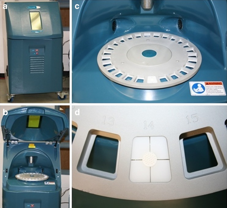
The LIBS technique is based on the atomic emission spectroscopy of laser-produced plasma (9). A laser pulse is focused on the surface of a sample to ablate a small amount of material. A few milligrams of the material are vaporized into a plume, leading to the ionization of its constituent atoms. Such atomic states decay by emission of radiation which is observed in the ultraviolet, visible, and near-infrared ranges. A spectrum composed of atomic lines and molecular bands is obtained by resolving the emitted light using an optical spectrometer. The constituent elements of a tablet (from coating or core) can thus be identified by analyzing the spectrum at wavelengths at which they emit light when decaying from high energy levels. Using this method, a relationship between the emission intensity and the concentration of the species of interest can be constructed using a simple univariate calibration curve, providing for a simple and efficient way to quantify a formulation composition. In this study, PharmaLIBS™250, an instrument manufactured by Pharmalaser, Inc. (10) (Fig. 1), was used for the LIBS analysis. It is divided into two compartments: the ablation chamber on the top is used to house the sample tray and laser guide. The bottom part contains a computer and a spectrometer, among other components. Neodymium-doped yttrium aluminum garnet (Nd:Y₃Al₅O₁₂) or Nd:YAG laser at 1,064-nm wavelength is passed through a beam sampler and a lens before it is redirected using a mirror onto the sample which is fixed in a placeholder on the carrousel. The light signal from the plasma produced as a result of sample ablation is transmitted through a fiber-optic bundle to the spectrometer and the CCD detector. The spectral data are transmitted to a computer which also controls the powder of the laser and monitors it using the signal from a Joule meter.

Fig. 1.

a PharmaLIBS™250 instrument. b The main door open showing the top compartment which contains a carousel and a laser guide above it. c Closer view of the carousel which has 26 slots in it. d Close-up of a slot in the carousel showing a tablet mounted using a holder which is machined to fit the tablet snugly

The main advantages of LIBS compared with other analytical techniques are its speed and the absence of a sample preparation step (e.g., digestion). The signal intensity value proportional to the amount of the element of interest can be compared for each site on a tablet (intra-tablet variability study) or as an average between several tablets for content uniformity evaluation. It can also be used, as in the present case, to assess the variability in thickness of the coating layer on the tablet. Successful application of LIBS for the analysis of pharmaceutical materials has been reported (11–16).

Data-Driven Statistical Models

Lack of first principles knowledge describing the behavior of granular systems has attracted significant attention to data-driven models for characterizing process performance. Hence, applications of such models are often treated as black box operations. The added advantage of methods such as the response surface method (RSM) is that their computational requirements are far less than mechanistic modeling methods. This also makes them good candidates for additional purposes such as real-time optimization and control. This study employs the RSM and kriging—two conceptually different data-based methods. The two methods provide outputs in different forms. The RSM produces non-interpolating surfaces (i.e., sum of squares error from a predefined function is minimized), while kriging produces interpolating surfaces (passing through all the experimental points). Both methods have attracted a significant amount of attention lately owing to their simplicity and computational efficiency (17–22). In this work, both methods are used to develop predictive models for the effects of spray rate, pan speed, exhaust temperature, and weight gain to the modified relative standard deviation (RSD). Kriging is an interpolating response surface method which is formed as a linear combination of basis functions. In the literature, through a comparison between RSM and kriging, it has been shown that in certain cases, fitted quadratic surfaces may not sufficiently capture the shape of the function (23). In addition, kriging has a statistical interpretation that allows the estimation of the potential prediction error. Kriging interpolation requires the tuning of very few parameter values which do not increase significantly when the number of input variables is large. The two methodologies are based on completely different principles, and by looking at their comparison, it becomes clear that kriging is more appropriate for cases where the response surface is expected to be non-convex and nonlinear, while RSM is more appropriate in cases where the output is expected to be a smooth and quadratic function. Finally, kriging may be more suitable in cases where the experimental data are not based on a carefully designed set of experiments since the prediction error is a quantitative measure for the identification of unexplored regions of the multivariable space. In this study, both these models have been used for the optimization and identification of the combination of operating conditions that minimize the coating thickness variability.

The Response Surface Method

RSM, a method first introduced by Box and Wilson in 1951 (24), is a tool that has been widely employed for the optimization of noisy processes. It is a local optimization technique whereby an optimum is achieved after sequential optimization of localized sampling-based models (25). There are three basic steps in the algorithm: (1) specification of a sampling set within the local region, usually accomplished by the design of experiment (DOE) tools; (2) construction of a local model centered at a nominal sampling point; and (3) model optimization with respect to the local region in order to determine the location at which process improvement is maximized. The spatial location of sampling points is an important aspect of RSM modeling since the sampling set should be representative of the entire experimental region and DOE tools are applied in order to address this issue. The experimental design is defined as the specification of a number of treatment levels for each input variable, the experimental units by which responses are measured, and the mechanism by which treatments are assigned to units.

For a problem containing n continuous input variables, an n-dimensional quadratic polynomial is used as the local model since quadratic behavior describes the mathematical geometry in the neighborhood of an optimum. Model accuracy can be improved if bilinear terms capturing the interaction effects between two inputs are also incorporated into the local model. A general second-order response surface model has the following form:

1

The indices i and j differentiate the input variables x_i and x_j, β₀, β_j, β_ij, and β_jj are model coefficients, and z represents the response that describes the predicted output behavior.

The Kriging Method

Kriging was first developed as an inverse distance weighting method to describe the spatial distribution of mineral deposits (26,27). This method has attracted a lot of attention recently due to its ability to model complex functions and to provide error estimates (21). In this method, the prediction f_k is expressed as a weighted sum of the observed function values at sampling points that fall within a set interval around the point that is predicted. The basic idea of kriging is that a function value for a sampling point located close to the test point is generally weighted more heavily in contrast to the function value corresponding to a sampling point located farther away. A lower weight is placed on function values whose sampling points are clustered together in order to minimize the possibility of generating biased estimates. Since a variance for each test point is also calculated, regions where subsequent sampling is required can be linked to a high variance at the regional points.

In the kriging method, the first step is the determination of variogram coefficients from an experimental sample set consisting of N sampling points. A variogram is a quantitative descriptive statistic that graphically characterizes data set roughness. The information obtained from it complements that which is obtained using histograms and other common descriptive statistics. In order to determine the variogram coefficients, (N)(N − 1)/2 squared function differences are obtained for each sampling pair. The squared function differences are then plotted with respect to the L²-norm sampling pair distance, as illustrated in Fig. 2a.

Fig. 2.

a Variogram model. b Semivariance. c Covariance plot

The best variogram model that should be used might not immediately be apparent. Data smoothing is used to improve the fit by replacing clustered scatterpoints falling within an interval [h_i − tol,h_i  + tol], tol being a certain tolerance, with average values defined as semivariances. The semivariance (γ(h)) is determined according to the equation:

2

where N(h) is the number of sampling pairs whose Euclidean distance falls within the range [h_i  − tol, h_i + tol]. Variogram model coefficients are then obtained from a regression of the semivariance scatterpoints to one of the five elementary types: spherical, Gaussian, exponential, power, or linear. The one whose least square error is the lowest is considered to be the type that best captures the trend of the semivariance. The covariance function which is a complementary function of the semivariance is used to calculate the Kriging weights (w_i) by solving the system:

3

where d_ij is the distance between sampling point x_i and sampling point x_j, and d_ik is the distance between sampling point x_i and test point x_k; λ is the Lagrangian multiplier of the optimization problem associated with the unbiased constraint. Similarly, Cov(d_ij) and Cov(d_ik) represent the modeled covariances between the sampled function data whose corresponding input vectors are a distance x_i–x_j or x_i–x_k apart, respectively. The kriging prediction f_k is then evaluated by the following form:

4

where w_i and f_i represent the weight and observed values at sampling point i, respectively. For each test point x_k, a variance is also obtained as follows:

5

where Cov(d_ik) corresponds to the right-hand side of Eq. 3.

MATERIALS AND METHODS

Tablets that were either fully coated or sampled at different stages of coating were used for analytical studies. The first sample, sample set A, contained 240 tablets from six production lots at 40 tablets per lot. The second sample, set B, contained 2,400 tablets from ten placebo lots with 240 tablets per lot sampled intermittently in sets of 40 at six different time points during a coating run. The third sample, set C, contained 120 tablets sampled after completed coating runs from three batches (40 tablets per batch), each with an increasing amount of API in them. A detailed study involving these three sets is presented in this paper. Another sample set, referred to as set M1, was used to develop the analytical method. Complete ANOVA and variance calculations for the method development study are not presented here, but can be found in Dubey et al. (28). Set M1 consisted of 100 tablets sampled from five production batches with 20 tablets per batch. This set was sampled from the same manufacturing plant, but using the old (pre-optimization) process. Hence, it can serve as an initial point for comparison of the overall variance in this study.

Development of LIBS-Based Analytical Method

This section describes the method development process for obtaining data from the LIBS instrument (intensity levels) and expressing it into quantitative measures of tablet coating thickness. The tablet coating was known to consist of titanium dioxide (TiO₂), and Ti gives a clearly identifiable peak in the emission spectrum at a wavelength of 521 nm. Hence, the intensity of Ti signal was chosen as an indicator of the coating. Spectra were collected at 19 sites per tablet, with 30 shots per site. A pattern of a central spot, surrounded by three concentric hexagons, was used to interrogate the entire tablet surface. Figure 3 shows the spatial distribution of the sites analyzed across the tablets, including the numbering scheme used to identify the sites.

Fig. 3.

Schematic description of site distribution on LIBS-analyzed tablets

The Ti signal intensity is high in the initial shots, but it drops as the laser pulses dig through the coating, indicating that the material ablated in the lower layers contains a lesser amount of coating material. The intensity decays slowly with the increasing number of shots. In order to determine a representative measure of coating thickness, a number proportional to the point where the Ti signal decays to 50% of its maximum was chosen. There were 19 measurements of maximum intensity per tablet, one from each site. A half of the average maximum intensity value for each tablet was chosen as the indicator of the average coating thickness for the given tablet. In a plot with the number of laser shots along the x-axis and signal intensity on the y-axis, the number of shots required to reach this average half-intensity was computed using a linear interpolation technique. While the shots are always in integral numbers, the interpolated number could be a value between two successive shots. This number was chosen as a representative of the coating thickness of the given tablet.

The details of the analytical method development and optimization can be found in (28). This study aims to build upon those findings. In summary, there were four main conclusions. First, the 19 locations on the tablet can be clubbed into three position zones. The first zone contained the central position and the six surrounding positions forming an innermost hexagon. The second zone comprised the six positions in the intermediate hexagon, and the third zone consisted of the outermost six locations, again in a hexagonal pattern (Fig. 3). Secondly, it was shown using statistical methods that there was no significant effect of the number of positions sampled, the frequency of data acquisition, the number of tablets chosen (as long as there were over 20 tablets), and that the three-zone method was justifiable. Hence, there are three position-related variables remaining within a tablet. The third inference was that the dome effect due to the curvature of the tablet can be easily modeled. The sites away from the tablet center exhibited consistently higher LIBS scores, but when corrected for the extra thickness that the laser would have to dig due to an oblique impact on the curved surface, it was found that the within-tablet variability that was detected by the technique was not significant. Hence, the perceived intra-tablet variability could be attributed to the curvature of the tablet. The fourth inference was that tablets from lots that were coated under the same conditions did not show statistically significant lot-to-lot variability, but they showed high tablet-to-tablet variability. This study proceeds using the sample sets A, B, and C, with the first two sets being used for systematic DOE while the third one for validation.

Statistical Model

As a starting point, the coating thickness score was expressed as:

6

where Y is the measured coating thickness score, μ is the mean coating thickness score, P is the effect of the radial position, L is the effect of the lot (batch), PL is the position–lot interaction, T is the effect of individual tablets nested within lots, PT is the position–tablet interaction, and ε is the error term, containing all other possible effects. Since the tablets are nested within lots, no three-way PLT interaction is possible in this model.

RESULTS: APPLICATION OF QbD PRINCIPLES FOR PROCESS OPTIMIZATION

First Analytical Study and Method Validation

Six different lots (sample set A) were manufactured under conditions detailed in Table I, and 40 tablets were analyzed from each lot. The variables manipulated in the study were the size of the pan and the load size (which are confounded), the coating thickness, and the type of coating. A summary of results for the entire data set is presented in Table II. Expected mean square (EMS) expressions were constructed using standard techniques.

Table I.

Conditions for Lots Used in the First Set of Designed Experiments Using Sample Set A

Lot no.	Coating type	Target coating weight (%)	Coating pan diameter (in.)	Load (kg)	RSD
8	Opadry II	2.50	60	270	9.51
9	Opadry II	4.50	60	265	10.90
10	Opadry II	4.50	19	15	11.53
11	Opadry II	4.50	19	15	10.07
12	Opadry II	7.50	19	15	7.63
13	Opadry II + HPMC clear coat	4.5 + 1% = 5.5%	19	15	9.93

Table II.

Summary of Calculations for the Data from Sample Set A

Source	Symbol	Fixed or random?	Levels	DOF	Sum of squares (SS)
Position	P i	F	3	2	1,486.39
Lot	L j	F	6	5	16,263.42
Position–lot interaction	PL ij	F	18	10	78.51
Tablets (within lots)	T k(j)	R	238	232	4,758.70
Position–tablet interaction	PT ik(j)	R	417	464	1,632.20
Error	ε m(ijk)	R	4,522	3,808	12,559.12
Totals				4,521	36,778.34

The complete ANOVA for this data set is shown in Table III. Significant position and tablet effects were detected, confirming this source of variability. As expected, since lots were manufactured using different conditions, a significant effect of lots was detected; the P × L interaction was also significant, while the P × T interaction was not.

Table III.

Complete ANOVA of Sample Set A Evaluating the Statistical Significance of All Main Effects and Interactions

Source of variation	SS	df	MS	F	Criteria	p value	F crit.
Between positions (P)	1,486.39	2	743.2	211.27	MS_P/MS_PT	5.82e−66	3.02
Between lots (L)	16,263.42	5	3,252.68	158.58	MS_L/MS_T	9.39e−73	2.25
Between tablets (nested within lots, T)	4,758.7	232	20.51	6.22	MS_T/MS_E	1.19e−140	1.16
Position–lot interaction (P × L)	78.51	10	7.85	2.23	MS_PL/MS_PT	0.015	1.85
Position–tablet interaction (P × T)	1,632.2	464	3.52	1.07	MS_PT/MS_E	0.17	1.12
Error	12,559.12	3,808	3.3
Total	36,778.34	4,521

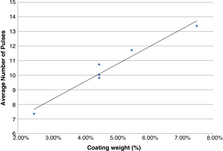
Since the lots contained different amounts of coating, the average LIBS scores for each lot to the amount of coating applied to each lot was compared. Figure 4 plots the lot average LIBS scores against the percent coating weight gain. The mean LIBS score for each lot correlates linearly and very closely to the amount of coating applied to each lot, providing validation to the analytical method. The analytical method is not only sensitive to the effects of processing conditions on different lots but also produces scores in agreement with the amount of coating imparted.

Fig. 4.

Correlation between the mean LIBS score (averaged for each lot) and the amount of coating (in weight gain percent) applied to each lot

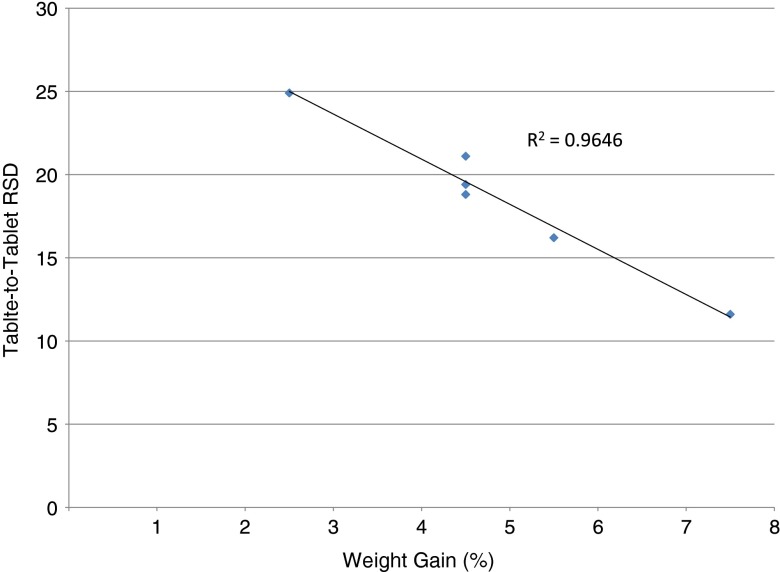
The target coating weight gains for each lot are shown in Table I. An important observation from Fig. 4 was that the correlation between LIBS scores and coating weights does not cross the origin; rather, as shown by the equation displayed in the figure, the intercept with the y-axis occurs at Y = 4.55 shots for 0% weight (no coating). This is a characteristic of the LIBS-based analytical technique. To account for this offset, the RSDs of the average LIBS score for each lot were calculated with a subtraction of a 4.55 constant factor from the mean for each lot. The results displayed in Fig. 5 were thus obtained, indicating a clear decrease of the RSD with increasing weight gain.

Fig. 5.

Tablet-to-tablet RSDs correlate very closely to the inverse of the weight gain

Looking back at the ANOVA in Table III, the effect of position can be explained as the result of the dome effect. As shown by Dubey et al. (28) using the same tablets, instrument, and settings, the thickness encountered by the laser beam when striking at positions away from the center (i.e., the top of the dome) is related to the angular positioning of the spot. Hence, there is perceived intra-tablet coating thickness variability. When the lot averages for each position were plotted as a function of the angular coordinate, excellent correlation was obtained for each percentage coating weight gain. Hence, most of the observed intra-tablet coating variability can be attributed to the dome effect.

Thus, the main effect that remains to be examined is the tablet-to-tablet component of the variance. As a first step in this direction, process simulations using DEM (29) were performed to study the effect of spray pattern, pan fill level, and pan speed on the coating uniformity in the O’Hara coating pan. In summary, the DEM results showed that the axial uniformity of the spray pattern is the most important phenomenon affecting the exposure of individual tablets to the spray zone. Since axial gradients in spray can only be mitigated by transport and mixing in the axial direction (the slowest mixing mode), other parameters that improve axial mixing also have an appreciable effect. The model predicted that better uniformity should be observed for longer process times, higher fill levels and higher rotational speeds. Complete details of this DEM study can be found in (5). While discussion of the modeling is outside the scope of this paper, these outcomes should be kept in mind as the analysis advances further.

Effect of Process Parameters on Tablet-to-Tablet Coating Thickness Variability

To characterize the effect of coating process parameters on variance components, another sample set (B) was collected from a series of designed experiments. Ten lots were manufactured using the conditions detailed in Table IV, and 240 tablets were analyzed for each lot at six sampling times (total 2,400 tablets). Samples were tested in sets of 40 taken from six time points for each lot, corresponding to weight gains of approximately 0.27%, 0.55%, 1.1%, 2.2%, 4.4%, and 6%. Three values of the spray rate were used—S, 1.25S, and 1.5S g/min—corresponding to a low, medium, and a high value of the variable, respectively. The exhaust temperature was measured and grouped into three groups: T to T + 2 (low), T + 3 to T + 5 (medium), and T + 6 to T + 8°C (high). Similarly, the pan speeds were: P, P + 2, and P + 4 rpm (low, medium, high, respectively).

Table IV.

Experimental Conditions Examined in Sample Set B

Run no.	1	2	3	4	5	6	7	8	9	10
Spray rate (g/min)	Medium	Medium	High	High	Low	Low	High	High	Low	Low
Exhaust temperature (°C)	Medium	Medium	High	High	Low	Low	Low	Low	High	High
Pan speed (rpm)	Medium	Medium	High	Low	Low	High	High	Low	Low	High
Sampling points	Weight gain (%)
1	0.29	0.29	0.27	0.27	0.28	0.28	0.27	0.27	0.28	0.28
2	0.58	0.59	0.53	0.53	0.55	0.55	0.53	0.53	0.55	0.55
3	1.15	1.17	1.07	1.07	1.11	1.11	1.07	1.07	1.11	1.11
4	2.30	2.35	2.13	2.13	2.22	2.22	2.13	2.13	2.22	2.22
5	4.61	4.69	4.27	4.27	4.44	4.44	4.27	4.27	4.44	4.44
6	6.00	6.00	6.00	6.00	5.99	5.99	6.00	6.00	5.99	5.99

An overall ANOVA was conducted for the data at a 6% weight gain. Since every lot was manufactured using a different set of manufacturing conditions, the variable “Lot” was treated as a fixed-level variable. The results (Table V) show that all three main effects (positions, lot, tablets) were significant, while no interactions were significant. The effect of position accounted for ∼15% of the total variance and correlated directly to the angular coordinate of the position (R² = 0.88). The effect of lots was significant and was attributed to the differences in process parameters used to manufacture each lot. However, lot-to-lot differences accounted for only ∼3.5% of the total variance. Finally, the effect of tablets within lots was also highly significant and also accounted for ∼15% of the total variance.

Table V.

Overall ANOVA Analysis of Sample Set B

Source of variation	SS	df	MS	F	Criteria	p value	F crit.
Between positions (P)	4,001.16	2	2000.58	548.4	MS_P/MS_PT	0.00	3.0
Between lots (L)	1,425.28	9	158.36	8.87	MS_L/MS_T	0.00	1.9
Between tablets (nested within lots, T)	6,964.05	390	17.86	4.89	MS_T/MS_E	0.00	1.12
Position–lot interaction (P × L)	72.37	18	4.02	1.1	MS_PL/MS_PT	0.345	1.61
Position–tablet interaction (P × T)	2,619.35	780	3.36	0.92	MS_PT/MS_E	0.935	1.09
Error	23,347.29	6,400	3.65
Total	38,429.50	7,599

Effect of Coating Weight Gain

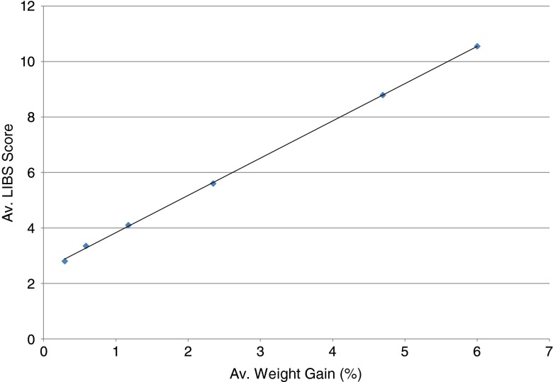
Figure 6 shows the average LIBS score for all ten lots combined as a function of the average weight gain for each sampling point. The increase is linear, and an extremely high degree of correlation is observed for the pooled data. This result compares favorably with a previously published study by Mowery et al. (16). However, as before, the LIBS score shows a systematic bias; rather than intersection with the origin, the average thickness score shows an intercept at 2.664 laser shots for a zero weight gain.

Fig. 6.

Average of the LIBS thickness score, averaged across ten lots

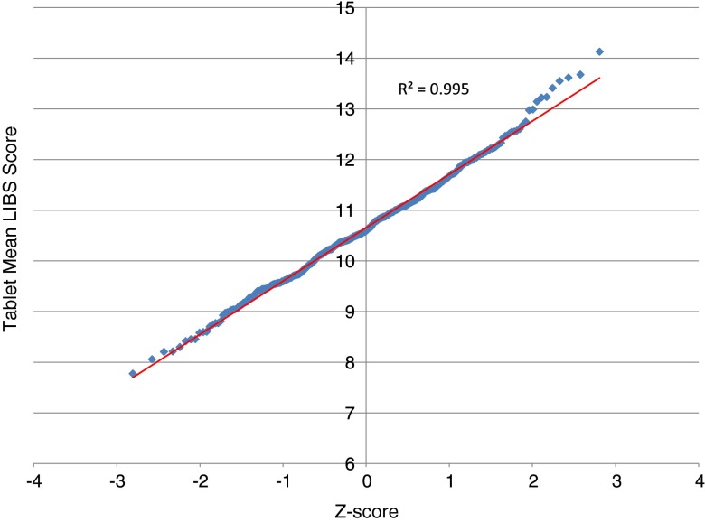
The degree of normality of the pooled tablet-averaged scores was tested before the tablet-to-tablet variability was analyzed. The results are shown in normal probability coordinates in Fig. 7 for a single data set of 400 tablets from all lots, all corresponding to a 6% weight gain. The results are extremely close to a normal distribution (R² ∼ 0.997), indicating that any measure of distribution breadth based on variance (i.e., the RSD) is an appropriate and sufficient quantification of the entire distribution.

Fig. 7.

Tablet-averaged thickness scores, pooled for ten lots, show an extremely close fit to a normal distribution

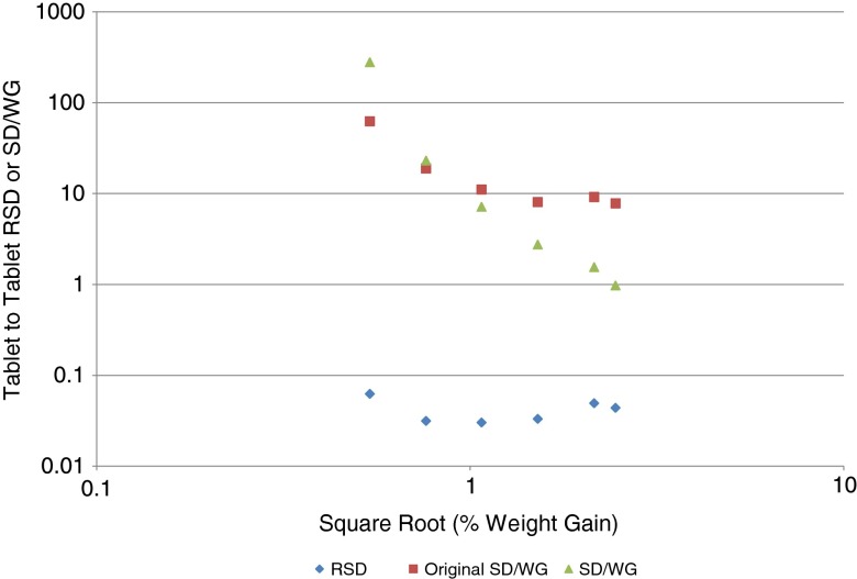
It has been shown in previous studies that the tablet-to-tablet coating variability is inversely proportional to the square root of weight gain (28) or coating time (3,6,30). In this study, the evolution of the RSD as a function of square root of weight gain for all lots is displayed in Fig. 8. Initially, the RSD was obtained using the usual definition, i.e., the SD was normalized by the mean of the set. This procedure yields the blue diamonds in Fig. 8 showing that the RSD decreased only slightly with increasing coating weight. This lack of agreement with the expected behavior was entirely due to the bias in the mean score, which artificially decreases the value of the RSD at low weight gain values. The same data, when normalized using the weight gain instead of SD, show a weak correlation, as displayed by the maroon squares in Fig. 8. To correct for background signal, which has an even higher impact for low coating weights, a constant value of 2.664 shots from the mean was subtracted. The corrected SD/WG shows a good correlation with weight gain, as shown by the green triangles in Fig. 8.

Fig. 8.

RSD of the tablet-averaged LIBS scores vs. average weight gain. Blue diamonds display results obtained when the RSD is normalized using the mean LIBS score averaged across all lots. Green triangles correspond to results obtained when the RSD was normalized by a modified mean score after the bias is subtracted from the mean LIBS score. Maroon squares correspond to results obtained when the RSD was normalized using the weight gain

Effects of Pan Speed, Spray Rate, and Temperature

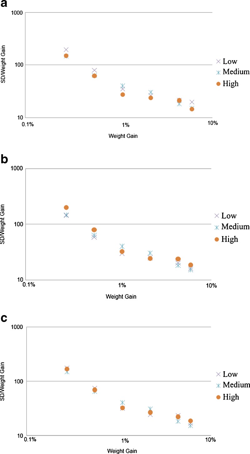
The effect of the pan speed was quantified by pooling all the tablet-averaged LIBS scores corresponding to the same (approximate) weight gains. The results show (Fig. 9a) that, in general, for higher speed, lower values of the SD/WG were observed, indicating that tablet-to-tablet variability decreased with increasing speed. This is in agreement with previously published studies (4,6). However, the effect of pan speed was small compared with other effects (i.e., the effect of weight gain) within the chosen range of speed. The effect of spray rate (Fig. 9b) was also similarly relatively small. A general trend was clear in the data (in agreement with expectations) that the lower spray rate yields slightly more homogeneous results (smaller RSDs). Again, this observation is consistent with other published data (3). Figure 9c shows the effect of temperature. The results indicate that over the range of temperatures examined, the effect was small, if any.

Fig. 9.

Effect of pan speed, spray rate, and temperature on RSD of tablet-averaged LIBS scores

PREDICTIVE MODELING USING DATA-DRIVEN METHODS

Model Validation

When using data-driven statistical methods, it is always important to validate the robustness of the models that are based on a number of fitted parameters. Leave-one-out cross-validation methodology is an iterative procedure during which one observed sample is “left out” at each step and a new model is constructed based on the reduced sampled set. If the sampling set is inadequate for the specific region or there are major outliers in the sampling set, then the removal of one point should not affect the new model parameters. This can be verified by simply using the new reduced sampling set-based model in order to predict the left-out sample (for which the real output is known). A commonly used diagnostic test that can provide a quick evaluation of the robustness and validity of a data-driven model is a plot of the actual function value vs. the cross-validated prediction. If the model is good, the points should show a good fit on a 45° line (22). A quantitative measure of the goodness of fit is the mean least squares error of the predicted left-out points vs. their actual values with respect to the function f(x) = x. The procedure of cross-validation is carried out for 50% of the experimental points which are randomly taken out of the sampling set.

Development of Predictive Models

The ability to produce input–output mappings using data-driven approaches not only allows the construction of a predicted output surface as a function of the input variables but also enables the identification of optimum operating conditions in order to satisfy a specific objective. Four parameters that affect the modified RSD were identified as the spray rate (x₁), pan speed (x₂), temperature (x₃), and weight gain (x₄).

These four variables were used in the response surface model from Eq. 1 (j = 4). However, a quadratic term is only included for variable x₄ (Eq. 7) based on the current experimental design. The optimized parameter values (b_j and b_ij) are shown in Table VI. The optimization was performed in General Algebraic Modeling System (31), where the objective of the optimization problem is the minimization of the least square of the error between predicted and experimental values. Based on the obtained quadratic response surface, a new optimization problem was formed for minimizing the predicted RSD subject to the input variables which were constrained within their experimentally tested ranges. The optimal combination of input variables was found to be:

Table VI.

Optimized Quadratic Response Surface Parameters for Eq. 7 Using Four Input Variables Based on the Experimental Data of Table VII

Parameter	Value
b 0	5.935
b 1	−0.220
b 2	−0.321
b 3	−1.170
b 4	−1.231
b 12	0.216
b 13	0.679
b 14	−0.065
b 23	−0.294
b 24	0.051
b 34	0.288
b 44	0.109

This suggests that in order to minimize the output variability, the process should be operated at minimum spray rate (in agreement with the analytical study), maximum pan speed, and low temperatures where the weight gain is relatively high. The inference that higher speed results in lower RSD is also in agreement not only with the analytical but also the DEM-based modeling study.

However, the input variable ranges had very different scales. The spray rate was in terms of hundreds of grams per minute, the temperature was varied within an 8°C window, and the pan speed was in terms of numbers <10 rpm. Thus, all input variables were normalized to a [0 1] range by division with their maximum level value. The logarithmic transformation of the output was found to be the most appropriate way to generate the data-driven response surface models. An average error of prediction value of 7.87% was obtained when a second-order response surface model was fitted to the experimental data shown in Table VII. Figure 10 shows a comparison between the actual and the predicted RSD. The quadratic response surface equation had the following form:

7

Table VII.

Experimental Data (60 Data Points) Used for the Development of the Data-Driven Method

Spray rate	Pan speed	Exhaust temperature	WG	RSD/WG
Medium	Medium	Medium	0.276	141.2201
Medium	Medium	Medium	0.551	57.391
Medium	Medium	Medium	1.103	42.49853
Medium	Medium	Medium	2.206	32.14512
Medium	Medium	Medium	4.412	16.77561
Medium	Medium	Medium	5.998	12.09731
Medium	Medium	Medium	0.276	137.8366
Medium	Medium	Medium	0.551	64.00527
Medium	Medium	Medium	1.103	30.74885
Medium	Medium	Medium	2.206	24.52377
Medium	Medium	Medium	4.412	17.97682
Medium	Medium	Medium	5.998	18.0915
High	High	High	0.276	180.9221
High	High	High	0.551	65.5858
High	High	High	1.103	26.26155
High	High	High	2.206	24.42879
High	High	High	4.412	21.83489
High	High	High	5.998	18.50271
High	Low	High	0.276	195.5087
High	Low	High	0.551	92.76363
High	Low	High	1.103	35.19413
High	Low	High	2.206	28.27531
High	Low	High	4.412	18.91655
High	Low	High	5.998	20.08049
Low	Low	Low	0.276	165.6004
Low	Low	Low	0.551	66.24541
Low	Low	Low	1.103	32.55265
Low	Low	Low	2.206	25.27056
Low	Low	Low	4.412	18.25478
Low	Low	Low	5.998	17.76121
Low	High	Low	0.276	141.8786
Low	High	Low	0.551	58.99649
Low	High	Low	1.103	25.57197
Low	High	Low	2.206	24.91249
Low	High	Low	4.412	18.05353
Low	High	Low	5.998	12.18082
High	High	Low	0.276	175.1925
High	High	Low	0.551	74.8951
High	High	Low	1.103	30.97355
High	High	Low	2.206	22.7638
High	High	Low	4.412	26.18948
High	High	Low	5.998	13.32663
High	Low	Low	0.276	213.3678
High	Low	Low	0.551	95.66086
High	Low	Low	1.103	35.96868
High	Low	Low	2.206	24.99163
High	Low	Low	4.412	22.07419
High	Low	Low	5.998	16.80901
Low	Low	High	0.276	150.5171
Low	Low	High	0.551	60.74419
Low	Low	High	1.103	35.69729
Low	Low	High	2.206	24.72072
Low	Low	High	4.412	20.455
Low	Low	High	5.998	15.85795
Low	High	High	0.276	113.6789
Low	High	High	0.551	45.54255
Low	High	High	1.103	23.5984
Low	High	High	2.206	24.07998
Low	High	High	4.412	20.41084
Low	High	High	5.998	14.75096

Fig. 10.

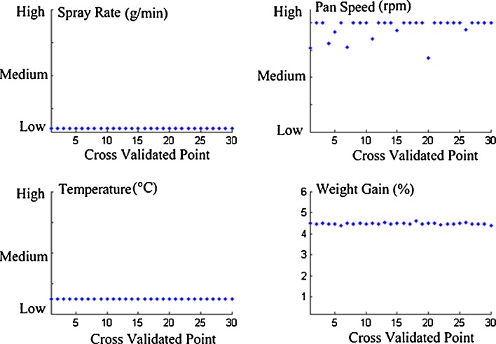
Predicted optimal operating conditions for each iteration of the leave-one-out cross-validation procedure based on the RSM model

In order to test the robustness of the model, leave-one-out cross-validation for a randomly selected portion of the data set was performed. The procedure involved the deletion of one observation at each iteration and the calculation of the model parameters based on the reduced data set. The left-out point was predicted based on the reduced data set model and its real value was compared with the predicted one, resulting in an error value. The overall average error of leave-one-out cross-validation was calculated as the mean squared error of all cross-validation iterations and was equal to 13.44%. In addition, the optimization problem was solved at every iteration based on the model obtained by the reduced data set in order to verify that the optimal operating conditions were not affected by the left-out observations (Fig. 10). Based on the value of the mean squared cross-validation error and taking into account the inherent noise present in the data, it was concluded that there were no major outliers in the data since the model parameters were not significantly affected when observations were randomly removed. This can also be verified by Fig. 10, where it is shown that the optimal conditions do not change significantly in any of the produced models. In fact, the only variable that was shown to be more sensitive was the pan speed, but in all cases, the models predict optimal performance at high values of this variable.

Next, an analogous model was built using kriging methodology. Due to the interpolating nature of kriging algorithm, different steps need to be taken for developing a kriging-based model for the modified RSD as well as for the optimization and validation of the model. Since kriging uses the actual experimental values for observed combinations of input variables, the only way of validating the model is by choosing a subset of the data as the training set and leaving the remaining observations as the test set. In order to eliminate any biased results, this procedure was performed several times for different randomly selected training sets. In each run, the training set comprised 40 points while the remaining 20 (Table VII) were used for calculating the average error of prediction of the model. This procedure eliminates the need for cross-validation of the model since the produced models are based on different data sets in every run.

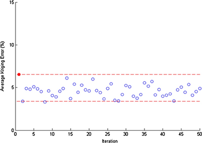
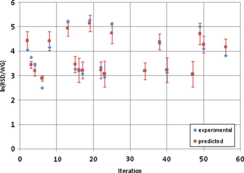
After 50 random simulations, the average kriging error of prediction for the 20 test points did not exceed the maximum value of 6.53% (Fig. 11). The predicted modified RSD is plotted against the actual values of the experimental data for the identified worst case (average kriging error = 6.53%) in Fig. 12. The advantage of using the kriging method for providing error estimates for each calculated prediction becomes obvious here as the majority of the experimental values are found to fall within the interval of the kriging uncertainty.

Fig. 11.

Average error (%) of kriging models based on 40 random training samples in each of the 50 iterations

Fig. 12.

Predicted vs. real model output using kriging model

Optimization based on kriging modeling is also very different from the methodology followed for RSM-based models. In this case, a closed-form expression of the output with respect to the input variables is not available, and hence, gradient-based optimization techniques cannot be applied. Optimization based on interpolating black box methods is based on direct search methods where the algorithm uses its feature of providing kriging variance in order to identify regions of high uncertainty which have not been sufficiently sampled. Once the algorithm converges, the optimal values of the covariance function parameters are used to calculate the predicted output over a fine grid of the input variable space. Finally, the minimum observed output is identified as the optimal. The optimal operating conditions identified by this procedure were the following:

Except for the pan speed which was predicted to have a lower optimal value, the kriging-optimized variables agree with the ones identified by the RSM.

Prediction of the Design Space

The concept of design space was formally introduced in 2005 (32,33) by the International Society of Pharmaceutical Engineering as one of the building blocks of the Product Quality Lifecycle Implementation initiative. In simple terms, it is the area of the parametric space within which an acceptable product can be produced. The identification and graphical representation of process design space is critical for locating not only the feasible but also the optimum operating variable ranges and design configurations. In Boukouvala et al. (34), the mapping of the design space of pharmaceutical processes was achieved using the ideas of process operability and flexibility under uncertainty. Optimal process design under uncertainty was defined as a rigorous formulation in the 1980s (35), where the effects of parameters that contain considerable uncertainty on the optimality and feasibility of a chemical plant were studied. The objective of solving such problems was to ensure optimality and feasibility of operation for a given range of uncertain parameter values by identifying a measure of the size of the feasible region of operation.

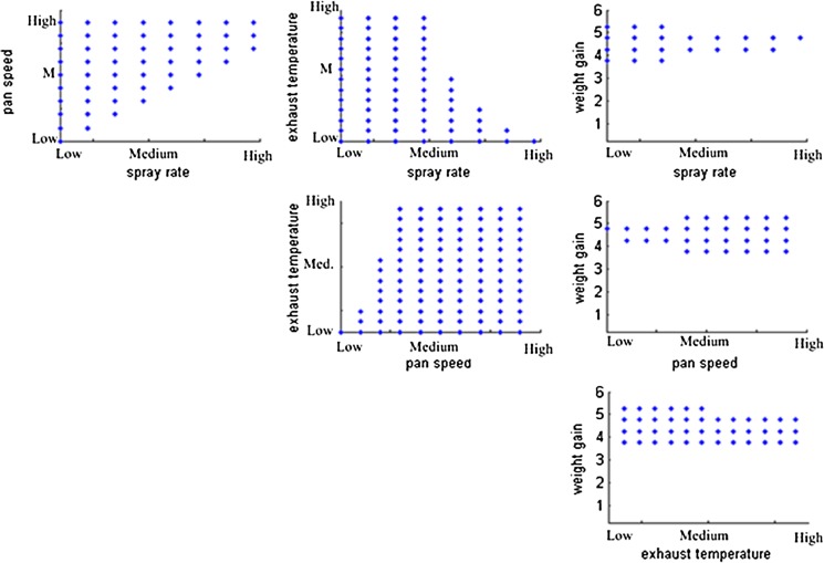
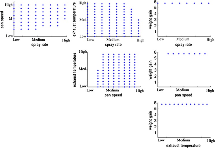
For the current study, the RSM and kriging can be used to identify the maximum deviations of the input variables that result in acceptable process variability. For example, if a maximum value of ln(RSD/WG)_max = 2.65 is considered to be the upper bound of acceptable variability, Figs. 13 and 14 illustrate the predicted acceptable regions of input variables that will result in equal to or lower than this bound.

Fig. 13.

Design space of coating process predicted by RSM model for

Fig. 14.

Design space of coating process predicted by kriging model for

With this analysis, it can be concluded that low weight gains lead to an increase in the output variability of the process since feasible operation is achieved for a small subset of the entire range of this variable. In addition, this analysis shows that regions where pan speed is very low while the spray rate is at its maximum value should be avoided.

VALIDATION AND EVALUATION OF THE QbD-BASED STUDY

Analysis of Validation Batches

Three batches, corresponding to potencies of p1, p2, and p3 (milligrams of active ingredient) were analyzed (sample set C). Each lot was manufactured under standard conditions and then coated using the modified coating process with the optimal process parameters determined in this study. A summary of results for the entire data set is presented in Table VIII. EMS expressions were constructed using standard techniques and used subsequently to compute variance components.

Table VIII.

Summary of Calculations for the Validation Data Set

Source	Symbol	Fixed or random?	Levels	DOF	Sum of squares (SS)
Position	P i	F	3	2	732.62
Lot	L j	F	3	2	290.79
Position–lot interaction	PL ij	F	9	4	70.83
Tablets (within lots)	T k(j)	R	120	117	1,838.98
Position–tablet interaction	PT ik(j)	R	360	234	746.88
Error	ε m(ijk)	R	2,280	1,920	6,056.58
Totals				2,279	9,736.69

The complete ANOVA for this data set is shown in Table IX. As in previous studies, all three main effects (positions, tablets, lots) were found to be statistically significant. Error accounted for approximately 70% of total observed variance. The effect of tablets (within lots) was by far the largest systematic effect, accounting for about 15% of the total observed variance. The effect of position (within tablets) was also quite large and accounted for about 11% of the total observed variability. As expected, since different coatings are applied to each lot, a statistically significant effect of the lots was also detected, although the contribution of the lots was a bit below 4% of the total observed variance (and essentially identical to that observed for the designed experiments using placebo tablets of sample set B). The P × L interaction was also statistically significant, although it contributed only about 1% of the total observed variance.

Table IX.

Complete ANOVA of Validation Data Set Evaluating the Statistical Significance of All Main Effects and Interactions

Source of variation	SS	df	MS	F	Criteria	p value	F crit.
Between positions (P)	732.62	2	366.31	114.76	MS_P/MS_PT	1.85E−35	3.03
Between lots (L)	290.79	2	145.4	9.25	MS_L/MS_T	1.86E−04	3.07
Between tablets (nested within lots, T)	1,839.00	117	15.72	4.98	MS_T/MS_E	7.89E−53	1.23
Position–lot interaction (P × L)	70.84	4	17.71	5.55	MS_PL/MS_PT	2.77E−04	2.41
Position–tablet interaction (P × T)	746.88	234	3.19	1.01	MS_PT/MS_E	0.44	1.17
Error	6,056.58	1,920	3.15
Total	9,736.69	2,279

Among the two large systematic main effects, tablets (within lots), and positions (within tablets), the latter can again be explained by examining the effect of the curvature of the tablet dome. Once again, when the lot averages for each position were plotted in terms of the geometric correction factor, excellent correlation was obtained for each coating thickness, demonstrating that the effect of position within tablets is caused by the increased thickness that the laser beam must cross when it intersects the coating at an angle due to the curvature of the tablet dome.

The degree of normality of the deviations with respect to the lot mean were tested in a similar fashion as it was done for sample set B. It was found that the results were extremely close to a normal distribution (with a R² ∼ 0.98), indicating that any measure of distribution breadth based on variance (e.g., the RSD) is an appropriate quantification of the breadth of the entire distribution of tablet-averaged scores for each lot.

Comparison of Validation and the Pre-validation Batches

In order to assess the effectiveness of this process improvement exercise, the RSD and the SD/WG index for each lot from the pre-validation sample set B and the validation set C were computed (Table X). Both RSD and SD/WG results were found to lie within the range observed in the designed placebo experiments, demonstrating the robustness of the new coating process. Moreover, for all three lots containing API, the results for both indices average lower than the mean of each index for the placebo lots, indicating that efforts to optimize the process were successful and that the new coating process was optimized (within the limitations of statistical methods). In order to provide an appropriate context for the degree of variability reduction achieved by the optimization of the process, the RSD of LIBS scores was compared for all data sets collected in the study.

Table X.

Summary of Tablet-to-tablet Variability Results

Lot	RSD	SD/WG
B1	0.068	13.197
B3	0.103	19.736
B3	0.102	20.185
B4	0.117	21.906
B5	0.102	19.376
B6	0.067	13.288
B7	0.073	14.538
B8	0.103	18.337
B9	0.083	17.300
B10	0.080	16.092
C1	0.093	19.012
C2	0.075	14.233
C3	0.083	16.012

Lots B1–B10 belong to sample set B and lots C1–C3 to sample set C

Evolution of Tablet-to-Tablet RSD over the Whole Study

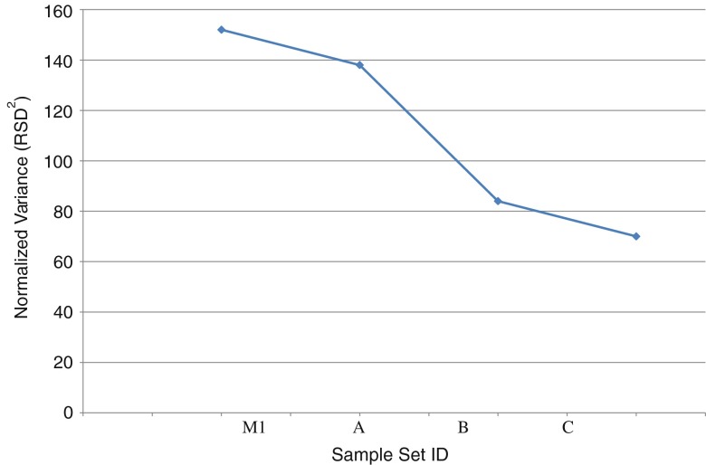
As the QbD-based study was carried out, the coating variability was systematically decreased. The highest variability (largest LIBS RSD) was observed during the initial trials. Information from the sample set M1 from a previous study (28) can also be included for comparison. During these trials, the coating process was characterized, and an initial DOE was conducted to examine the effect of coating parameters. A significantly lower variability was observed for sample set A which examined the effect of using different coating thicknesses and/or different types of coatings. Variability was decreased further during the main DOE conducted as part of the project (sample set B). When these experiments were conducted, the lessons learned during the previous sets of experiments were used to select the coating material and the sets of conditions to be examined, and the design space was marked. These also provided inputs for the data-driven methods that were subsequently used to optimize the process. Finally, the confirmation lots (sample set C) were, as expected, close to the lower end of the range of values observed during the main DOE of sample set B.

The significance of the progressive reduction in variability achieved during the sequence of experiments conducted in this study is further highlighted in Fig. 15, which shows the evolution of the normalized variance (RSD^2), averaged for all lots in each set. The initial sample set M1, which was from production lots from the old process, showed the highest variance. The variance was subsequently reduced for sample sets A, B, and C. Ultimately, it was decreased by more than half.

Fig. 15.

Normalized variance averaged over all lots in each sample set used in this study. The variability was reduced to less than a half of its original value as a result of the development of optimized process

CONCLUSION

These results reported here demonstrate that the new coating process optimized by this QbD study was robust and produced consistent results. The new set of results obtained for the three lots of commercial product confirms all of the main observations previously reported:

1. The main source of avoidable variability in the coating process was tablet-to-tablet (within lot) variability which, as previously demonstrated, was caused by mixing limitations of the coating pan.

2. Variability due to position (within tablets) was simply an artifact of the curvature of the tablet dome.

3. A small variability component due to the lot-to-lot differences was also detected, but accounted only for a few percent of the total variability.

Moreover, the process conditions selected in the previous studies (using sample sets A and B) were used successfully to manufacture commercial products having a coating variability that was consistent (slightly lower) with the average of the placebo lots, thus confirming that the conditions selected as the result of the DOE study indeed minimize coating variability (within the constraints of the approved manufacturing process). Overall comparison showed that the variance was reduced by more than half by optimizing coating composition, coating thickness, and the parameters of the coating process.

References

- 1.Roggo Y, Jent N, Edmond A, Chalus P, Ulmschneider M. Characterizing process effects on pharmaceutical solid forms using near-infrared spectroscopy and infrared imaging. Eur J Pharm Biopharm. 2005;61(1–2):100–110. doi: 10.1016/j.ejpb.2005.04.005. [DOI] [PubMed] [Google Scholar]
- 2.Kandela B, Sheorey U, Banerjee A, Bellare J. Study of tablet-coating parameters for a pan coater through video imaging and Monte Carlo simulation. Powder Technol. 2010;204(1):103–112. doi: 10.1016/j.powtec.2010.07.024. [DOI] [Google Scholar]
- 3.Joglekar A, Joshi N, Song Y, Ergun J. Mathematical model to predict coat weight variability in a pan coating process. Pharm Dev Technol. 2007;12(3):297–306. doi: 10.1080/10837450701247442. [DOI] [PubMed] [Google Scholar]
- 4.Sahni E, Chaudhuri B. Experiments and numerical modeling to estimate the coating variability in a pan coater. Int J Pharm. 2011;418:286–296. doi: 10.1016/j.ijpharm.2011.05.041. [DOI] [PubMed] [Google Scholar]
- 5.Dubey A, Hsia R, Saranteas K, Brone D, Misra T, Muzzio FJ. Effect of speed, loading and spray pattern on coating variability in a pan coater. Chem Eng Sci. 2011;66(21):5107–5115. doi: 10.1016/j.ces.2011.07.010. [DOI] [Google Scholar]
- 6.Pandey P, Katakdaunde M, Turton R. Modeling weight variability in a pan coating process using Monte Carlo simulations. AAPS PharmSciTech. 2006;7(4):E2–E11. doi: 10.1208/pt070483. [DOI] [PubMed] [Google Scholar]
- 7.Sahni E, Yau R, Chaudhuri B. Understanding granular mixing to enhance coating performance in a pan coater: experiments and simulations. Powder Technol. 2011;205(1–3):231–241. doi: 10.1016/j.powtec.2010.09.019. [DOI] [Google Scholar]
- 8.Tobiska S, Kleinebudde P. A simple method for evaluating the mixing efficiency of a new type of pan coater. Int J Pharm. 2001;224(1–2):141–149. doi: 10.1016/S0378-5173(01)00742-6. [DOI] [PubMed] [Google Scholar]
- 9.Miziolek AW, Palleschi V, Schechter I. Laser-induced breakdown spectroscopy (LIBS): fundamentals and applications. Cambridge: Cambridge University Press; 2006. [Google Scholar]
- 10.Pharmalaser. www.pharmalaser.com.
- 11.Green RL, Mowery MD, Good JA, Higgins JP, Arrivo SM, McColough K, et al. Comparison of near-infrared and laser-induced breakdown spectroscopy for determination of magnesium stearate in pharmaceutical powders and solid dosage forms. Appl Spectrosc. 2005;59(3):340–347. doi: 10.1366/0003702053585354. [DOI] [PubMed] [Google Scholar]
- 12.Madamba MC, Mullett WM, Debnath S, Kwong E. Characterization of tablet film coatings using a laser-induced breakdown spectroscopic technique. AAPS PharmSciTech. 2007;8(4):E103. doi: 10.1208/pt0804103. [DOI] [PMC free article] [PubMed] [Google Scholar]
- 13.Mukherjee D, Cheng MD. Characterization of carbon-containing aerosolized drugs using laser-induced breakdown spectroscopy. Appl Spectrosc. 2008;62(5):554–562. doi: 10.1366/000370208784344451. [DOI] [PubMed] [Google Scholar]
- 14.St-Onge L, Archambault JF, Kwong E, Sabsabi M, Vadas EB. Rapid quantitative analysis of magnesium stearate in tablets using laser-induced breakdown spectroscopy. J Pharm Pharm Sci. 2005;8(2):272–288. [PubMed] [Google Scholar]
- 15.St-Onge L, Kwong E, Sabsabi M, Vadas EB. Quantitative analysis of pharmaceutical products by laser-induced breakdown spectroscopy. Spectrochim Acta Part B At Spectrosc. 2002;57(7):1131–1140. doi: 10.1016/S0584-8547(02)00062-9. [DOI] [Google Scholar]
- 16.Mowery MD, Sing R, Kirsch J, Razaghi A, Béchard S, Reed RA. Rapid at-line analysis of coating thickness and uniformity on tablets using laser induced breakdown spectroscopy. J Pharm Biomed Anal. 2002;28(5):935–943. doi: 10.1016/S0731-7085(01)00705-1. [DOI] [PubMed] [Google Scholar]
- 17.Boukouvala F, Dubey A, Vanarase AU, Ramachandran R, Muzzio FJ, Ierapetritou MG. Computational approaches for studying the granular dynamics of continuous blending processes—II: Population balance and data-based methods. Macromol Mater Eng. 2011. doi:10.1002/mame.201100054.
- 18.Boukouvala F, Muzzio FJ, Ierapetritou MG. Predictive modeling of pharmaceutical processes with missing and noisy data. AICHE J. 2010;56(11):2860–2872. doi: 10.1002/aic.12203. [DOI] [Google Scholar]
- 19.Davis E, Ierapetritou M. A kriging-based approach to MINLP containing black-box models and noise. Ind Eng Chem Res. 2008;47(16):6101–6125. doi: 10.1021/ie800028a. [DOI] [Google Scholar]
- 20.Davis E, Ierapetritou M. A kriging based method for the solution of mixed-integer nonlinear programs containing black-box functions. J Glob Optim. 2009;43(2):191–205. doi: 10.1007/s10898-007-9217-2. [DOI] [Google Scholar]
- 21.Jia Z, Davis E, Muzzio F, Ierapetritou M. Predictive modeling for pharmaceutical processes using kriging and response surface. J Pharm Innov. 2009;4(4):174–186. doi: 10.1007/s12247-009-9070-6. [DOI] [Google Scholar]
- 22.Jones DR, Schonlau M, Welch WJ. Efficient global optimization of expensive black-box functions. J Glob Optim. 1998;13(4):455–492. doi: 10.1023/A:1008306431147. [DOI] [Google Scholar]
- 23.Jones DR. A taxonomy of global optimization methods based on response surfaces. J Glob Optim. 2001;21(4):345–383. doi: 10.1023/A:1012771025575. [DOI] [Google Scholar]
- 24.Box GEP, Wilson KB. On the experimental attainment of optimum conditions. J R Stat Soc Ser B Methodol. 1951;13(1):1–45. [Google Scholar]
- 25.Myers RH, Montgomery DC. Response surface methodology: process and product in optimization using designed experiments. New York: Wiley; 1995. [Google Scholar]
- 26.Cressie N. Statistics for spatial data (Wiley Series in Probability and Statistics) New York: Wiley-Interscience; 1993. [Google Scholar]
- 27.Isaaks E, Srivastava R. Applied geostatistics. New York: Oxford University Press; 1989. [Google Scholar]
- 28.Dubey A, Keyvan G, Hsia R, Saranteas K, Brone D, Misra T, et al. Analysis of pharmaceutical tablet coating uniformity by laser-induced breakdown spectroscopy (LIBS) J Pharm Innov. 2011;6(2):77–87. doi: 10.1007/s12247-011-9103-9. [DOI] [Google Scholar]
- 29.Dubey A, Sarkar A, Ierapetritou MG, Wassgren CR, Muzzio FJ. DEM based approaches for studying the granular dynamics of continuous blending processes. Macromol Mater Eng. 2011;296(3–4):290–307. doi: 10.1002/mame.201000389. [DOI] [Google Scholar]
- 30.Pandey P, Song Y, Kayihan F, Turton R. Simulation of particle movement in a pan coating device using discrete element modeling and its comparison with video-imaging experiments. Powder Technol. 2006;161(2):79–88. doi: 10.1016/j.powtec.2005.09.003. [DOI] [Google Scholar]
- 31.GAMS (General Algebraic Modeling System). http://www.gams.com/default.htm.
- 32.Garcia T, Cook G, Nosal R. PQLI key topics—criticality, design space, and control strategy. J Pharm Innov. 2008;3(2):60–68. doi: 10.1007/s12247-008-9032-4. [DOI] [Google Scholar]
- 33.Lepore J, Spavins J. PQLI design space. J Pharm Innov. 2008;3(2):79–87. doi: 10.1007/s12247-008-9034-2. [DOI] [Google Scholar]
- 34.Boukouvala F, Muzzio F, Ierapetritou M. Design space of pharmaceutical processes using data-driven-based methods. J Pharm Innov. 2010;5(3):119–137. doi: 10.1007/s12247-010-9086-y. [DOI] [Google Scholar]
- 35.Halemane KP, Grossmann IE. Optimal process design under uncertainty. AICHE J. 1983;29(3):425–433. doi: 10.1002/aic.690290312. [DOI] [Google Scholar]