Variation Transmission Model for Setting Acceptance Criteria in a Multi-staged Pharmaceutical Manufacturing Process

Abstract

Pharmaceutical manufacturing processes consist of a series of stages (e.g., reaction, workup, isolation) to generate the active pharmaceutical ingredient (API). Outputs at intermediate stages (in-process control) and API need to be controlled within acceptance criteria to assure final drug product quality. In this paper, two methods based on tolerance interval to derive such acceptance criteria will be evaluated. The first method is serial worst case (SWC), an industry risk minimization strategy, wherein input materials and process parameters of a stage are fixed at their worst-case settings to calculate the maximum level expected from the stage. This maximum output then becomes input to the next stage wherein process parameters are again fixed at worst-case setting. The procedure is serially repeated throughout the process until the final stage. The calculated limits using SWC can be artificially high and may not reflect the actual process performance. The second method is the variation transmission (VT) using autoregressive model, wherein variation transmitted up to a stage is estimated by accounting for the recursive structure of the errors at each stage. Computer simulations at varying extent of variation transmission and process stage variability are performed. For the scenarios tested, VT method is demonstrated to better maintain the simulated confidence level and more precisely estimate the true proportion parameter than SWC. Real data examples are also presented that corroborate the findings from the simulation. Overall, VT is recommended for setting acceptance criteria in a multi-staged pharmaceutical manufacturing process.

INTRODUCTION

Pharmaceutical manufacturing processes consist of a series of unit processes or unit operations, referred to as stages in this paper, to generate the active pharmaceutical ingredient (API). For example, a process starts with a chemical reaction and is followed by workup, filtration, and crystallization to isolate the API. The quality attributes of the API are affected by the earlier stages. To assure that the final drug product meets its quality requirement, the in-process control (IPC) and the API need to be controlled within their respective specified acceptance criteria.

Several works have been published for calculating acceptance criteria (1–3). These employ some type of a statistical interval (confidence, prediction, and tolerance) to incorporate process average and process variability. These works, however, are applied to only a single-unit operation. Methods applicable to a process with sequential unit operations are of interest.

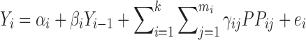
Per the ICH Q6A Justification of Specifications, one of the sources from which acceptance criteria may be established is relevant process development data. Process development usually entails exploratory screening, optimization, and robustness studies using factorial experiments. These design-of-experiments (DOEs) type of studies purposely vary input materials and process parameters relevant to a stage to determine their effect on the output. Separate DOE studies are typically performed at each stage for ease of execution. An example process development DOE scheme of a k-staged process is diagrammed in Fig. 1.

Fig. 1.

Diagram of sequential k-staged manufacturing process where separate DOE studies are performed at each stage. Notations: Y _i = monitored quality attribute (e.g., impurity level); PP _ij = jth process parameters (e.g., temperature, pressure) studied at ith stage; e _i = error at each stage

The monitored quality attributes are impurities which are either generated from side reaction of the reactants, transformed from one isomer to another, or carried across the stages as inert chemical species. For a well-defined pharmaceutical manufacturing process, the pathways that impurities follow across the stages are known. Hence, it is possible to track a particular impurity at each stage and infer empirical relationships between Y_i and Y_i−1 and/or PP_ij’s, whether the impurity remains untransformed or does undergo some chemical transformation.

Given a dataset generated from a scheme such as Fig. 1, the key question is how should variation from a previous stage be taken into account in setting acceptance criteria for subsequent intermediate stages and ultimately for the final stage? A simplified risk minimization strategy practiced in the industry is referred to in this paper as serial worst case (SWC) approach. This entails determination of maximum output level for Y_i that would be expected to be generated at stage i by calculating an upper limit of a statistical interval when input starting materials and process parameters are set at their worst-case settings. Since the monitored quality attribute is an impurity, the higher its output level, the “worse” it is from a safety perspective. The maximum (worst) expected output of stage i is then carried over as input material to stage i + 1 wherein again the process parameters are fixed at worst-case settings. This procedure is serially repeated from one stage to the next until the final kth stage, hence the name for the approach. The calculated upper limits of statistical intervals at intermediate and final stages are then used as basis for establishing IPC and API acceptance criteria. Although the SWC does result in deriving acceptance criteria with minimized risk of excursion, the calculated limits can be artificially high and may not reflect the actual process performance. An alternate, more realistic approach to SWC is needed to establish statistically-based acceptance criteria for each stage of the process.

Several papers studying variation in product quality attributes as it moves through multiple stages of manufacturing process have been published. The terminologies introduced and the particular industries the works have been applied to are: variance synthesis (4,5); stream of variation in automotive body assembly (6); variation transmission using autoregressive model in automobile manufacturing (7); variation propagation using state space model in machining processes (8); and variation transmission in ceramic tile manufacturing (9).

In this paper, the concept of variation transmission (VT) by (7) is combined with tolerance interval calculations as a proposed method to derive acceptance criteria for a multi-staged process. The method is presented in the context of having generated process development data using but not limited to factorial experiments at each process stage. The paper is subdivided into the following: (1) introduction of variation transmission model in a generalized k-staged process; (2) brief review of tolerance interval concept; (3) simulation study and real data examples to compare tolerance intervals calculated using SWC and the proposed VT.

METHODS

Variation Transmission in a k-Staged Process

Consider the diagram of a k-staged manufacturing process depicted in Fig. 1. At each stage, factorial DOE would have been performed during process development. Assuming the quality attribute of the output (Y_i) is linearly correlated to the input starting material (Y_i−1) and the process parameters (PP_ij’s), the multiple linear regression equation (Eq. 1) applies:

1

where subscript i refers to ith stage (i = 1, …, k); subscript j refers to jth process parameter in stage i (j = 1, …, m_i; where m_i is the number of process parameters studied at stage i); α_i is the intercept; β_i and γ_ij are the regression coefficients for Y_i−1 and PP_ij predictor variables, respectively. For the purpose of introducing the concept of variation transmission, the simple case where only Y_i−1 influences Y_i is first presented (i.e., γ_ij's = 0). This case may occur in a process robustness study wherein the ranges of the PP_ij’s are chosen such that varying the PP_ij’s within this range have no statistically significant effect on Y_i. The quality of the input starting material Y_i−1 almost always influences Y_i based on mass balance principles. Other cases where both Y_i−1 and PP_ij’s influence Y_i and also where neither influences Y_i will be presented later in the Real Data Examples section.

For the case considered in this section, it can be modeled by a simple linear regression:

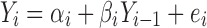2

with 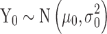. Equation 2 is an example of a first-order autoregressive model in which the distribution of Y_i depends only on Y_i−1 (10). The errors at each stage, e_i’s, are assumed to be independent of each other (recursive error structure) and normally distributed N(0,). The expected value and variance of Y_i are:

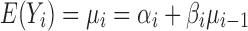3

4

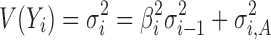
Equation 4 estimates variation transmitted through the i^th stage of the process. The first term () on the right-hand side is the variation transmitted to Y_i from stage i − 1, while the second term () is the variation added at stage i. The regression coefficient (β_i) is a measure of the extent of variation transmission. By using Eq. 4 recursively, the variation transmitted through the final kth stage can be generalized as:

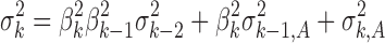5

Tolerance Interval

A tolerance interval is an interval expected to contain at least a specified proportion, p, of the population with a specified degree of confidence, (1 − α). Since tolerance interval estimates the capability limits of a process manufacturing products in large quantities (11), this type of interval is appropriate for setting acceptance criteria. An upper tolerance limit for a univariate linear regression model of the form shown in Eq. 6 (12) is used in this paper.

6

where is the predicted mean in vector notation of the ordinary least squares regression; k(x) is the tolerance factor which is dependent upon proportion p, confidence level (1−α, and sample size n), and can be calculated from (13) or obtained from statistical textbooks; S is an estimate of variability.

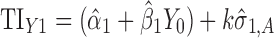
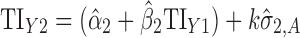
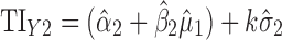
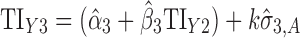
Applications of Eq. 6 to set acceptance criteria via SWC and VT differ slightly by virtue of how the respective methods work. To illustrate and contrast the difference, the resulting tolerance interval calculations for the two methods are written out for a k = 3 process in Table I. For example, using SWC at stage 2, the predicted mean 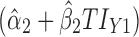is evaluated at the maximum output level of stage 1 (TI_Y1) but S used is variation contributed solely by stage 2 (). In essence, the variation from stage 1 is incorporated to stage 2 via the calculated TI_Y1 (i.e., the maximum or worst-case scenario from stage 1). 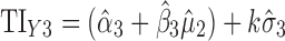Using VT at stage 2, the predicted mean 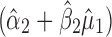is evaluated at the predicted mean of stage 1 but S used is the total variation transmitted up to stage 2 ().

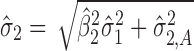Table I.

Tolerance Interval (TI) Calculations for k = 3 Staged Process Using Serial Worst-Case (SWC) and Variation Transmission (VT)

Stage	SWC	VT
1
2
3

Simulation Study

A computer simulation experiment is performed to compare tolerance limits at each of process stages calculated using SWC and VT. The process considered is Fig. 1 with k = 3 and no effects of process parameters PP_ij’s (i.e., γ_ij's = 0). Conditions of varying extent of variation transmission (β_i = 0.1 or 1.0) and varying stage variability (σ_i,A = 0.1 or 1.0) are simulated. The selected (β_i,σ_i,A) combination is assumed to apply to each of the k stages. Since this work is presented in the context of having performed some process development studies, sample sizes (n = 10, 40, 80) are used. These values are typical number of experimental units performed during process development of a pharmaceutical drug. The simulated scenarios are tabulated in Table II.

Table II.

Simulated Scenarios Varying β _i and σ _1,A with Each Combination Sampled at n = 10, 40, and 80

Extent of variation transmission (β i)	Variability at each stage (σi,A)
	0.1	1.0
0.1
1.0

The specific steps followed in the simulation are: (a) specify arbitrary values for intercepts (α_i = 1) and input starting material quality (Y₀ = 5) in Eq. 2; (b) select (β_i,σ_i,A) combination applied to each of the k stages; (c) simulate Y_i’s at each (β_i,σ_i,A) combination using the RANNOR random number generator function in SAS taking into account the autoregressive relationship (i.e., output in stage 1 becomes input for stage 2, etc.); (d) perform ordinary least squares regressions (Eq. 2) at each stage; (e) construct upper one-sided (p = 0.99, 1 − α = 0.95) tolerance intervals at each stage for SWC and VT using formulas in Table I; (f) repeat steps c to e 2,000 times.

The metrics for the simulation study are: (1) confidence coefficient, which is empirically derived as the fraction of constructed tolerance intervals that correctly contain at least the true proportion (p = 0.99) of the simulated population and (2) average tolerance interval length. The method with confidence coefficient that is closer to the true confidence level and with shorter average tolerance interval length is deemed the better method.

Real Data Examples

Three cases of varying scenarios on extent of variation transmission and on stage variability as well as different number of process stages and correlation (or lack thereof) of Y_i with Y_i−1 and/or PP_ij’s are presented to further illustrate the simulation findings. The description of each case is presented in more detail in the next section along with the calculations using Eq. 1 and the formulas in Table I.

RESULTS

Simulation Study: Confidence Coefficient

Figure 2 presents the simulated confidence coefficients as process stage progresses (Y₁→Y₂→Y₃). The results are given for the two methods (SWC and VT) and three sample sizes (n = 10, 40, 80) tested. The four panels correspond to the different (β_i,σ_i,A) combinations. Using the normal approximation to the binomial, if the true confidence level is 0.95, a simulated confidence level based on 2,000 iterations has only a 0.025 probability of being less than 0.94. A reference line at 0.94 is drawn in the plots.

Fig. 2.

Plot of simulated confidence coefficients as process stage progresses (Y₁→Y₂→Y₃) for method (VT=variation transmission, SWC=serial worstcase) and sample size (n) in each of (β _i,σ _i,A) simulated scenarios. The reference line at 0.94 is the simulated confidence level

At low extent of variation transmission (β_i = 0.1) for both levels of variability (σ_i,A = 0.1 and 1.0), the simulated confidence coefficients for SWC at smaller sample sizes (n = 10 and 40) fall further below 0.94 as stage progresses (Fig. 2, upper left and right panels). VT approaches the simulated confidence level for all σ_i,A and n levels as stage progresses. At large size (n = 80), the confidence level of both methods improve and become comparable to each other.

At high extent of variation transmission (β_i = 1.0), SWC exceeds 0.94, approaching or even reaching 1.0 for both σ_i,A levels as stage progresses (Fig. 2, lower left and right panels). VT also exceeds 0.94 at low variability (σ_i,A = 0.1) but not as severely as SWC; the exceedance is attenuated as sample size is increased. At high variability (σ_i,A = 1.0), VT effectively maintains simulated confidence level with results approaching 0.94 as stage progresses for all sample sizes.

Simulation Study: Average Tolerance Interval Length

Figure 3 presents the average tolerance interval lengths as process stage progresses. The average TI length is re-scaled by subtracting from it the “true” 99th percentile of the simulated N() population. The smaller this difference is, the more precise the estimate of the true proportion parameter. This re-scaling makes it easier to graphically compare the two methods across the four (β_i,σ_i,A) simulated scenarios.

Fig. 3.

Plot of average tolerance interval lengths (less the true proportion p values of the simulated population) for process stages progresses (Y₁→Y₂→Y₃) for method (VT variation transmission; SWC serial worst case) and sample size (n) in each of (β _i,σ _i,A) simulated scenarios

At low extent of variation transmission (β_i = 0.1), the average TI lengths of SWC are longer than VT although only slightly (Fig. 3, upper left and right panels). The difference from the true proportion parameter is widened as stage progresses, more so with SWC than with VT. As expected, increased sample size improves the precision of the estimates. These trends are similar between σ_i,A = 0.1 and σ_i,A = 1.0, only differing by an order of magnitude in the Y-axis scale.

At high extent of variation transmission (β_i = 1.0), the average TI lengths of SWC are drastically much longer than VT (Fig. 3, lower left and right panels). The disparity between the two methods becomes even more pronounced as stage progresses. Again, improved precision is achieved by increasing sample size. Just like in β_i = 0.1 scenario, trends between σ_i,A = 0.1 and σ_i,A = 1.0 are similar in β_i = 1.0 scenario except for scaling of Y-axis by an order of magnitude.

Taking together the results of the confidence coefficients and average TI lengths for the scenarios tested, SWC is verified to be a conservative method—it exceeds the simulated confidence level, even reaching 1.0 as stage progresses, and it gives longer tolerance limits thus less precise estimates of true proportion parameter. In contrast, VT is more effective in maintaining the simulated confidence level and provides more precise estimates of true proportion parameter. These contrasts in performance are especially observed when extent of variation transmission is high and process stage variability is also high.

Real Data Examples

In this section, real data examples are presented to further illustrate setting acceptance criteria using the SWC and VT methods. The data comes from actual retrospective historical data and/or prospective DOE studies that have been slightly modified for proprietary reasons. The identities of the chemical impurities measured in these studies are blinded for confidentiality.

Case 1 is a three-staged process wherein the output of a stage, Y_i, appears to be influenced solely by its input material, Y_i−1. This is similar to the hypothetical case considered in the simulation, only the estimates of σ_i’s and σ_i,A’s vary from stage to stage. Case 2 is a two-staged process wherein Y_i also appears to be influenced by Y_i−1. In addition, two process parameters PP₂₁ and PP₂₂ also appear to influence the output of stage 2, Y₂. Case 3 is a three-staged process wherein for stages 1 and 3, the outputs Y₁ and Y₃ appear to be correlated with their input materials, Y₀ (upon log-transformation) and Y₂, respectively. However for stage 2, neither its starting material Y₁ nor any of its PP_ij’s appear to influence the output Y₂. This may occur, for example, in robustness studies wherein the goal is to demonstrate that within the selected range of the input parameters, there is no significant effect on the output. This may also occur when the process is inherently variable such that any signal due to systematic sources of variation could not be detected.

In all of these three cases, when systematic sources of variation (Y_i−1 and PP_ij’s) appear significant, they are modeled in Eq. 1 as fixed effects. Modeling them as random effects is probably more reflective of how these factors behave in real applications. For example, the chemical impurity of interest Y₀ contained in the starting material supplied by a vendor is likely distributed as a normal random variable, . Likewise, the setting at which a process parameter PP_ij is actually operated may also have some random distribution (e.g., uniform or triangular) within its normal operating range. The scope of the current paper, however, is on how to account for random sources of variation in each stage, σ_i,A. Therefore, in evaluating the expected stage output Y_i, the systematic sources of variation are fixed at their worst-case scenarios (Y₀ at input material specification; PP_ij at the setting that gives the highest level of Y_i), in keeping with the overall risk minimization strategy. For accounting for the stochastic nature of the systematic sources of variation, the reader is referred to these papers (3,14,15).

Figures 4, 5, and 6 show the experimental data, the predicted mean of the fitted regression model (solid line generated from Eq. 1), and the constructed tolerance intervals (dashed lines) using formulas in Table I for SWC and VT methods. Estimates of the variation at each stage (), and the total transmitted variation up to a stage ( from Eq. 4) are also presented. Reference lines on X-axis are drawn corresponding to the levels at which to evaluate the input material Y_i−1 to obtain the Y_i tolerance interval.

Fig. 4.

Case 1 example: High extent of variation transmission, low-stage variability. Three-staged process where Y_i’s appear correlated solely with respective Y_i−1’s

Fig. 5.

Case 2 example: Low extent of variation transmission, low-stage variability. a Stage 1 of a two-staged process where Y₁ appears correlated with Y₀. b Stage 2 of a two-staged process where Y₂ appears correlated with Y₁ and process parameters PP₂₁ and PP₂₂

Fig. 6.

Case 3 example: Variable (low, “zero,” and high) extent of variation transmission, low-stage variability. Three-staged process where Y₁ and Y₃ appear correlated with respective input materials but Y₂ does not appear correlated with Y₁ or any PP_2j’s

For case 1 (Fig. 4), the slopes of the regression lines at each stage are all large . This exemplifies the high extent of variation transmission scenario in the simulation. The variabilities at each stage are relatively small . The reference line in stage 1 (Fig. 4a) is 0.15 corresponding to Y₀ specification. The predicted mean 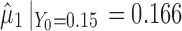and the calculated TI = 0.24. This value is identical for both SWC and VT methods at stage 1 since it is assumed that the total transmitted variation up to the first stage equals the variation at that stage (i.e., ). For stage 2 (Fig. 4b) using SWC, Y₁ is evaluated at the worst-case output of stage 1 (TI_{Y1_SWC} = 0.24) and using variation at stage 2 (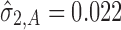), the calculated TI_{Y2_SWC} = 0.35. For stage 2 using VT, the Y₁ is evaluated at the predicted mean output of stage 1 (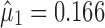) and using the total transmitted variation up to stage 2 (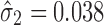), the calculated TI_{Y2_VT} = 0.31. This procedure is repeated for stage 3 (Fig. 4c) and the calculated TI’s are 0.46 and 0.36, for SWC and VT, respectively. For this case scenario of high extent of variation transmission with low stage variability, the calculated TI at the final process stage using VT is 0.1 lower than SWC.

For case 2 (Fig. 5), the slopes are relatively small and stage variability are also small 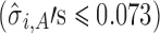.The reference line in stage 1 (Fig. 5a) is 6.5 corresponding to Y₀ specification. At stage 2, PP₂₁ and PP₂₂ along with Y₁ appear to significantly influence Y₂. Figure 5b groups the observations according to the PP_2j settings (center points for historical data and low–high factorial settings for DOE data). PP_2j’s are fixed at settings that give the highest value of Y₂ (PP₂₁ = 16 and PP₂₂ = 0.75) as a risk minimization strategy. For stage 2 using SWC, Y₁ is evaluated at the worst-case output of stage 1 (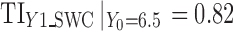) and using , the calculated TI_{Y2_SWC} = 0.22. For stage 2 using VT, Y₁ is evaluated at the predicted mean output of stage 1 (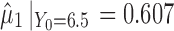) and using 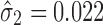, the calculated TI_{Y2_VT} = 0.20. In this case of low extent of variation transmission and low stage variability, the calculated TI at the final process stage using VT is 0.02 lower than SWC.

For case 3 (Fig. 6), the ′s are 0.043, 0, and 0.924 for stages 1, 2, and 3, respectively, and the ′s are all relatively low (≤0.025). The reference line in stage 1 is LN(1) = 0 corresponding to natural-log-transformation of Y₀ = 1 specification (Fig. 6a). The apparent lack of correlation between Y₂ and Y₁ or with any of the process parameters PP_2j’s () in stage 2 (Fig. 6b), may occur, as discussed earlier, during process robustness studies or in a highly variable process. With , the total transmitted variation up to stage 2 using Eq. 4 is . This means that has “zero” extent of transmission into stage 2 and only comprises . Since the regression model in stage 2 is no better than the overall mean of the Y₂ observations (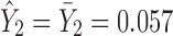), the predicted mean will be 0.057 whether Y₁ is evaluated 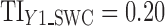at or at 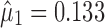. Because of this and since , then the calculated TI_Y2 = 0.12 is identical for SWC and VT. For stage 3 (Fig. 6c) using the SWC method, Y₂ is evaluated at the worst-case output of stage 2 (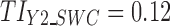) and using 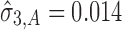, the calculated TI_{Y3_SWC} = 0.17. For stage 3 using the VT method, Y₂ is evaluated at the predicted mean output of stage 2 (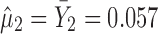) and using 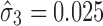, the calculated TI_{Y3_VT} = 0.14. For this case of variable (low, “zero,” and high) extent of variation transmission with low stage variability, the calculated TI at the final process stage using VT is 0.03 lower than SWC.

DISCUSSION

Simulation results indicate that at low extent of variation transmission, at both low- and high-stage variability, and at small sample size, SWC performs poorly relative to VT. With increased sample size, the two methods become practically comparable with the average TI lengths of VT only slightly shorter than those of SWC. This trend is corroborated in the low (or variable) extent of variation transmission, low-stage variability real data examples (cases 2 and 3); VT is only slightly shorter than SWC by 0.02 or 0.03.

The superiority of VT over SWC is especially demonstrated in simulation of high extent of variation transmission and high stage variability. In this scenario, VT more effectively maintains the nominal confidence level and more precisely estimates the true 99th percentile parameter than SWC. The real data example case 1 involves high extent of variation transmission but with low-stage variability. The calculated tolerance limit for VT is 0.1 shorter than SWC and had the stage variability been high, this difference would have been much bigger.

An impurity is introduced in the pharmaceutical drug manufacturing process either from its initial level in the starting material or as a by-product of chemical reaction. If the efficiency of the process in reducing/eliminating this impurity is low (i.e., poor purging), its level going into a stage will approximately remain unchanged from the previous stage. This chemical specie mass balance is a manifestation of high extent of variation transmission which is not uncommon in pharmaceutical drug manufacturing process. The high extent of variation transmission, specifically coupled with high-stage variability, is where the industry practice method SWC performs particularly poorly as shown in the simulation. Setting impurity control limits that exceed the true capability of the process, even by small exceedances, as can be the case using SWC, may have critical implications on the safety of the drug in human patients. Thus, it becomes more imperative to set a more realistic basis for setting control limits by properly accounting for transmission of variation through a multi-staged process using the VT method.

Generalization of Calculation Procedure

The variation transmission concept presented in the simulation and real data examples can be generalized into practical, procedural steps for setting acceptance criteria: (1) screen for the pertinent sources of variations at each stage of a multi-staged process using available studies (e.g., process development data including retrospective historical database and/or prospective factorial DOE studies), (2) estimate effects of systematic and random sources of variation at each stage from the fitted regression model (Eq. 1), (3) estimate total variation transmitted up to stage i using Eq. 4, (4) calculate upper one-sided tolerance limits for each quality attribute at each stage using Eq. 6 wherein S is estimated from step 3, (5) use the calculated tolerance limits as the basis for setting acceptance criteria in the intermediate and the final stages.

CONCLUSION

This paper addresses the question of how variation in previous stages of a multi-staged pharmaceutical manufacturing process can be appropriately accounted for in subsequent stages. The end goal is establishing a method for setting statistically-based acceptance criteria for intermediate and final stages of the process. Computer simulations are used to compare serial worst case (SWC) and variation transmission (VT) approaches in terms of maintaining the simulated confidence level and estimating the true proportion parameter. When the extent of variation transmission is low, SWC performs poorly but with increased sample size, it is practically comparable with VT. When the extent of variation transmission is high and especially when stage variability is high, VT is the superior method. The real data examples which considered various cases of extent of variation transmission, stage variability, and apparent correlation (or lack thereof) of output with input and/or process parameters corroborate the findings from the simulation. Therefore, variation transmission (VT) approach is recommended for setting acceptance criteria in a multi-staged pharmaceutical manufacturing process.

REFERENCES

- 1.Seely RJ, Munyakazi L, Haury J. Statistical tools for setting in-process acceptance criteria. Biopharm. 2001;14(10):28–34. [PubMed] [Google Scholar]
- 2.Orchard T. Setting acceptance criteria from statistics of the data. Biopharm Int. 2006;19(11):34–46. [Google Scholar]
- 3.Burdick R, Gleason T, Rausch S, Seely J. Using tolerance intervals for setting process validation acceptance criteria. Biopharm International. 2007; June:40–46.
- 4.Morrison SJ. The study of variability in engineering design. Appl Stat (Royal Stat Soc). 1957;6(2):133–138. doi: 10.2307/2985509. [DOI] [Google Scholar]
- 5.Morrison SJ. Variance synthesis revisited. Qual Eng. 1998;11(1):149–155. doi: 10.1080/08982119808919220. [DOI] [Google Scholar]
- 6.Hu SJ, Koren Y. Stream-of-variation theory for automotive body assembly. CIRP Ann Manuf Technol. 1997;46(1):1–6. doi: 10.1016/S0007-8506(07)60763-X. [DOI] [Google Scholar]
- 7.Lawless J, MacKay R, Robinson J. Analysis of variation transmission in manufacturing processes—part I. J Qual Technol. 1999;2(31):131–142. [Google Scholar]
- 8.Huang Q, Zhou S, Shi J. Diagnosis of multi-operational machining processes through variation propagation analysis. Robot Comput Integr Manufac. 2002;18(3–4):233–239. doi: 10.1016/S0736-5845(02)00014-5. [DOI] [Google Scholar]
- 9.Heredia J, Gras M. Statistical estimation of variation transmission model in a manufacturing process. Int J Adv Manuf Tech. 2010;52:789–795. doi: 10.1007/s00170-010-2735-y. [DOI] [Google Scholar]
- 10.Greene, W. Econometric Analysis. 2nd ed. Prentice Hall. 1993.
- 11.Hahn, GJ, Meeker, WQ. Statistical intervals: a guide for practitioners. John Wiley & Sons, Inc. 1991.
- 12.Krishnamoorthy K, Mathew T. Statistical tolerance regions. Theory, applications, and computation. John Wiley & Sons, Inc. 2009.
- 13.Natrella, MG. Experimental Statistics, NBS Handbook 91, US Department of Commerce. 1963.
- 14.Diwekar UM, Rubin ES. Stochastic modeling of chemical processes. Comput Chem Eng. 1991;15(2):105–114. doi: 10.1016/0098-1354(91)87009-X. [DOI] [Google Scholar]
- 15.Johnson DB, Bogle DL. Handling uncertainty in the development and design of chemical processes. Reliab Comput. 2006;12(6):409–426. doi: 10.1007/s11155-006-9012-7. [DOI] [Google Scholar]