Early stages of the recovery stroke in myosin II studied by molecular dynamics simulations

Abstract

The recovery stroke is a key step in the functional cycle of muscle motor protein myosin, during which pre-recovery conformation of the protein is changed into the active post-recovery conformation, ready to exersice force. We study the microscopic details of this transition using molecular dynamics simulations of atomistic models in implicit and explicit solvent. In more than 2 μs of aggregate simulation time, we uncover evidence that the recovery stroke is a two-step process consisting of two stages separated by a time delay. In our simulations, we directly observe the first stage at which switch II loop closes in the presence of adenosine triphosphate at the nucleotide binding site. The resulting configuration of the nucleotide binding site is identical to that detected experimentally. Distribution of inter-residue distances measured in the force generating region of myosin is in good agreement with the experimental data. The second stage of the recovery stroke structural transition, rotation of the converter domain, was not observed in our simulations. Apparently it occurs on a longer time scale. We suggest that the two parts of the recovery stroke need to be studied using separate computational models.

Introduction

Myosin is a motor protein involved in the contractile movement of muscle filaments. Driven by the hydrolysis of adenosine triphosphate (ATP), the functional cycle of myosin head contains a series of steps consisting of conformational changes combined with binding to actin filaments and ATP.¹ Key among these steps are (1) the power stroke, a post-hydrolysis transition that occurs in actin-bound protein and results in force generation and (2) the recovery stroke, a transition that takes the protein back to its active state and occurs in ATP-bound state but when myosin is detached from actin. The end points of the recovery stroke are referred to as pre-recovery, M*, and post-recovery, M** states accordingly. The recovery stroke is reversible in myosin with bound ATP^2,3 as well as with the product of ATP hydrolysis, ADP and Pi,⁴ but occurs on a vastly different time scale for these two ligands. The equilibrium between two states is controlled by environmental factors including temperature and pressure.²

In this work we focus on myosin II, for which multiple crystallographic studies⁵ show that the differences between M* and M** structural states are limited to three areas, as illustrated in Figure 1. First, it is the ATP binding pocket, where switch II (SWII) loop can be either in open or close state. Second, it is the converter domain, which is strongly coupled to the lever arm, mediating contractile movement. And third, it is the relay helix that interfaces with both the converter domain and the SWII loop. It is believed that the SWII loop closure triggers a structural chain reaction that leads to the bending of the relay helix and rotation of the converter domain toward M** structural state. This transition was followed experimentally by observation of intrinsic fluorescence changes during temperature jump,^2,6 in electron paramagnetic resonance (EPR)³ and fluorescence resonance energy transfer (FRET) studies⁷ of myosin liganded with non-hydrolizable ATP analogs. While producing valuable structural information about M* and M** conformations, such as inter-residue distances,^3,7 such experiments however fall short of providing full microscopic detail.

Figure 1.

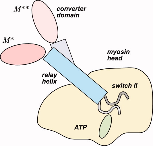
Cartoon explaining two alternative structural states of ATP-bound myosin: pre-recovery stroke state M* and post-recovery state M**. SWII loop is open in M* state. Its closure triggers a cascade of conformational changes that result in bending of the relay helix and rotation of the converter domain in M** state. [Color figure can be viewed in the online issue, which is available at wileyonlinelibrary.com.]

Alternative, theoretical methods are able to access atomic resolution directly and thus offer a competitive advantage. Much of our current understanding of the recovery step transition in myosin is based on computational studies at the atomic resolution, a large number of which have been conducted in the past several years.^4,8–17 Despite these recent efforts, however, an integrated and widely accepted view of how myosin functions remains elusive. Because of the large size of the protein, the observation of the recovery transition, occurring on millisecond time scale,³ directly in simulations is not possible at present. The longest simulations reported to date are limited to the 1–5 ns range.^11,12 To circumvent the long relaxation time problem, many studies employ biased sampling of conformations, either in the form of umbrella potential^14–17 or a pre-arranged reaction coordinate.^9,13 While efficient in generating transitions between two end points, these approaches employ approximations that may adversely affect the transition pathways.

In this work, we extend the microscopic simulations of myosin beyond their present scale. We report a series of long unbiased atomistic molecular dynamics simulations of M* and M** states at constant temperature in implicit and explicit solvent. The time scales of 10–50 ns and the number of generated trajectories in this work, 5–10, far exceed those reported previously. For the first time, in our simulations we observe spontaneous closure of SWII loop in trajectories started from the pre-recovery conformation M*. The dynamics of the ATP-binding pocket has a multi-state character with the stable open and closed conformations. Although the complete M*-to-M** transition was not seen in our simulations, structural signatures of its initial steps are consistent with experiment. In particular, the distances between K498 and A639 residues correlate well with the corresponding distances measured in EPR and FRET experiments.³ Taken together, our results support a multi-step model for the recovery stroke transition, in which SWII loop closure does not communicate to the converter domain immediately but rather is separated from it by a time delay.^13,15,16

Results

The quality of computational models is judged by comparison with experiment. In addition to atomic structures of myosin in two end-points of the recovery stroke, M* (pre-recovery stroke structural state), and M** (post-recovery stroke structural state), there are recent spectroscopic studies^7,18 reporting on structures and structural kinetics of myosin during M*–M** transition. The distance and distance distribution between labeled residues K498 and A639 in myosin liganded with non-hydrolizable ATP and ADP.Pi analogs were measured with pulsed EPR and FRET. Interprobe distance distribution exhibited two maxima which were interpreted as corresponding to myosin structural states M* and M**. We compare the results of our simulations with experimental results for K498:A636 distance, obtained from myosin atomic structures and the results of spectroscopic studies^7,18 to validate our computational approaches.

Dynamics of inter-residue distances in unbiased simulations

First, we test whether the two-state dynamics can be modeled directly in unbiased simulations without any assumptions on myosin intermediate states during M*–M** transition. The protein was modeled in atomic detail, using explicit solvent. The distance distributions between N_ζ atom of K498 and C_β atom of A639 observed in 50 ns aggregated simulations of M* and M** structural states are shown in Figure 2, together with experimental pulsed EPR data.⁷ The distribution functions are focused around the average values of 3.4 nm for M** state and 3.8 nm for M* state, in excellent agreement with experimental data. The average distance departs farther from its initial value in M* simulations than in M** simulations, indicating greater conformational freedom of the former structural state. In both M* and M** states there are no discernible signs of multi-state dynamics. Figure 2 thus suggests that on the time scale of the performed simulations, 50 ns in aggregate, myosin undergoes only local fluctuations with no conformational states sampled that could be relevant for the recovery stroke transition. It follows therefore that the model employing explicit solvent is too slow to yield qualitative agreement with experiment for the K498–A639 distance distribution.

Figure 2.

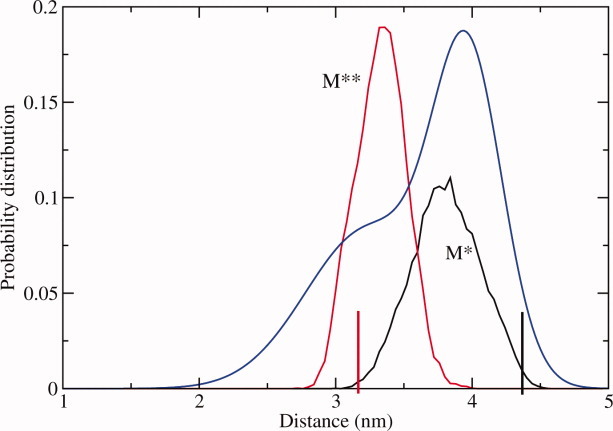
Probability distribution functions for the distance between N_ζ atom of K498 and C_β atom of A639 observed in explicit solvent simulations at T = 300 K. Vertical lines correspond to the initial values of the distance in crystallographic M* and M** states. Blue line is the experimental EPR interprobe distance distribution.⁷ [Color figure can be viewed in the online issue, which is available at wileyonlinelibrary.com.]

In order to make the model more computationally efficient it has to be simplified. First and most natural simplification concerns the treatment of the solvent. In contrast to explicit solvent, which treats every water molecule in atomic detail, implicit solvent represents the effect of water molecules through effective potentials acting on the protein. As a consequence, a large reduction in the total number of degrees of freedom in the simulated system is achieved. In the present work, simulations with implicit solvent model ran about five times faster than the equivalent explicit solvent model, allowing us to extend the total simulation time by that amount. Another benefit of treating solvent implicitly is accelerated conformational dynamics of the protein. In explicit solvents, the dynamics of solute molecules is controlled by the solvent's viscosity or internal friction. The magnitude of the friction is used as a parameter in implicit solvent simulations and thus can be varied to obtain faster or slower dynamics. We used the friction coefficient of 0.5 ps⁻¹.To estimate the resulting acceleration rate, we computed the diffusion coefficient for a methane molecule in implicit and explicit solvents for this friction coefficient at T = 300 K and all other conditions similar to our myosin simulations. The diffusion coefficient for methane molecule, measured in implicit solvent was 0.3 nm²/ps, and in explicit solvent was 0.005 nm²/ps, resulting in approximately 50 times slower dynamics. We thus estimate that our 50 ns implicit solvent simulations should be able to probe conformational transitions within myosin, such as loop closing, occurring on microsecond time scale in explicit solvent under equivalent thermodynamic conditions. One weakness of implicit solvent models is that they are built on a number of approximations that may or may not be accurate.¹⁹ The latest generation of implicit solvents, however, especially those based on generalized Born (GB) formalism, were shown to be of excellent quality.^19,20 We employ in this work the GB model developed by Onufriev et al.²¹ which yields electrostatic solvation energy in excellent agreement with the Poisson–Boltzmann equation.

The interprobe distance distribution functions obtained in implicit solvent simulations at T = 300 K are shown in Figure 3. The M* state distance distribution is in good agreement with the explicit solvent simulations, sharing both a similar unimodal shape and a similar position of the maximum probability. In M** simulations, the distance distribution is shifted toward larger distances. Importantly, neither M* nor M** distance distribution has a multi-modal nature, which is a characteristic of several alternative conformations sampled during the simulations. We thus conclude that even the longer scale implicit solvent simulations are not sufficiently long to reveal recovery stroke transition in myosin. In order to achieve even higher conformational dynamics, the common tool is to increase the temperature of the simulated system. If the transitions are controlled by a free energy barrier ΔF, their rate can be increased according to ΔF/kT ratio, where k is the Boltzmann constant. To test the efficiency of this tool in the present study, all simulations were repeated with the temperature set at T = 350 K. The resulting distribution functions are shown in Figure 3. Clear qualitative changes can be seen compared to T = 300 K. First, the distance distributions for M* and M** structural states become considerably broader. Second and most important, a multi-modal character of the distribution functions clearly emerges. Two maxima are observed for M* simulations and three maxima for M** simulations. The width of both M* and M** distance distributions is about the same, but their shapes are different. This is expected, as we do not believe that the equilibration has occurred in our simulations. We expect that the conformational ensembles sampled in both simulations have some overlap, but we do not anticipate a full convergence. We conclude that our simulations at T = 350 K qualitatively agree with the experiment regarding the distance between K498 and A639. Given that we use accurate protein and solvent models, myosin conformations sampled in our simulations are relevant to those obtained experimentally.

Figure 3.

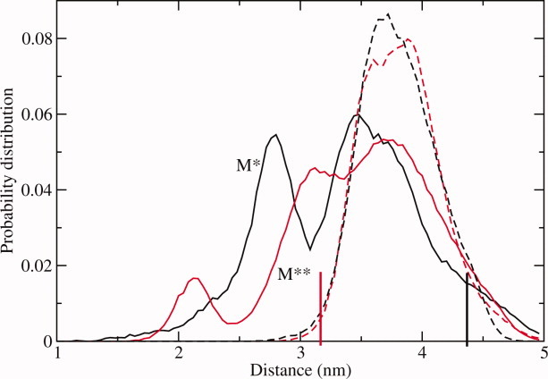
Same as Figure 2 but for implicit solvent modeling at T = 350 K, solid lines, and T = 300 K, broken lines. [Color figure can be viewed in the online issue, which is available at wileyonlinelibrary.com.]

Implicit solvent simulations reveal switch II loop closure

A hydrogen bond between nitrogen atom of G457 and P_γ atom of ATP is the hallmark signature of the post-recovery step conformation M** observed in crystallographic studies. It results from the loop spanning residues D454–I460 in pre-recovery stroke state M* moving closer to the ATP binding site and completing what is known as SWII closure. The closing event activates ATP hydrolysis^14,22,23 and was suggested to serve as a trigger that sets the recovery stroke in motion.⁹ Our simulations are perfectly suited to probe the early stages of this process. Figure 4 shows the distribution function of the distance between atoms G457:N and ATP:P_γ obtained in explicit solvent simulations of M** state where H-bond is present. The distribution is narrowly peaked around 0.42 nm with a small subpopulation at 0.36 nm, showing that the bond remains intact throughout the simulations. In contrast, the distribution obtained in implicit solvent at T = 300 K with M* initial structure, without the hydrogen bond present, shows four maxima all of which are located at distances greater than 0.5 nm. There is virtually no overlap with the reference distribution indicating that there are no hydrogen bonds formed in these simulations. Clearly, the simulations at low temperature are not able to observe SWII closure.

Figure 4.

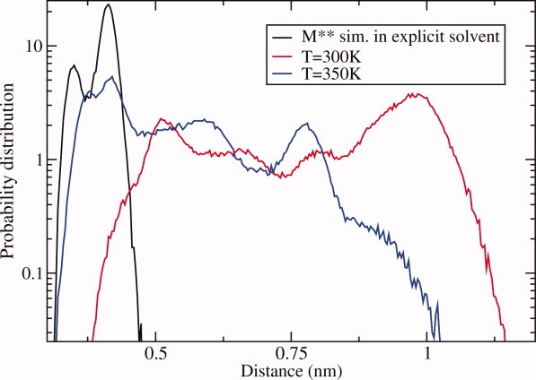
Distribution function of the distance between N atom of G457 and P_γ of ATP molecule. Black line: simulations in explicit solvent started from M** structural state with the SWII closed. Colored lines are for implicit solvent simulations started from M* state with the switch open. Red line: T = 300 K, blue line: T = 350 K. Spontaneous closure of the switch is seen at T = 350 K temperature only. [Color figure can be viewed in the online issue, which is available at wileyonlinelibrary.com.]

Higher temperatures accelerate conformational dynamics, increasing transitions probability. The distribution function obtained at T = 350 K in implicit solvent (Fig. 4) displays three maxima with the highest of them located at 0.42 nm. This is the same distance as in the reference distribution showing that the hydrogen bond was formed in these simulations. An analysis of all 10 trajectories revealed 6 events of SWII closure. One of these events was reversible, where H-bond creation was followed by H-bond breaking and subsequent re-establishment. Overall, the number of SWII closures is small suggesting that the free energy barrier controlling them is high. Additionally, the dynamics of the interatomic G457–ATP distance has multi-state character, as Figure 4 shows, where at least two minima are seen between open and closed states. Whether the multiplicity of the intermediate states is a consequence of the limited sampling in our simulations or it reflects the true nature of SWII closure remains to be studied. In the latter case, the dynamics of SWII loop will be defined by more than one free energy barrier, each potentially playing a unique role in the recovery stroke transition.

Correlation of events at the nucleotide binding pocket

This is the first time the spontaneous closure of SWII loop is observed in an unbiased simulation. As SWII closure leads to the recovery stroke, it is important to examine myosin conformations that accompany it. For that purpose, myosin conformations with G457:N-ATP:P_γ distance, less than 0.46 nm (the first minimum of SWII position probability distribution for T = 350 K implicit solvent simulation in Fig. 4), were collected at SWII-closed states and grouped into clusters. Clustering was done using mutual root-mean square deviation (RMSD) over C_α atoms of fragments G175–N188, N233–R238, S456–E459, and P_γ atom of ATP, all of which are located within 1 nm of ATP molecule and thus constitute the “nucleotide binding pocket.” One major family of structures that emerged from such clustering is shown in Figure 5 in comparison with the M** conformation determined experimentally. The two structures overlap almost perfectly with the mutual C_α RMSD of less than 0.1 nm.

Figure 5.

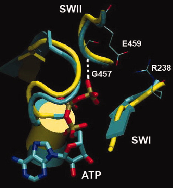
Conformation of the ATP binding pocket. Yellow: crystallographic M** structure, cyan: high-temperature implicit solvent simulations. Hydrogen bond between G457 and ATP and a salt bridge between E459 and R238 are observed in both structures. [Color figure can be viewed in the online issue, which is available at wileyonlinelibrary.com.]

An important structural motif, observed in the ATP binding pocket is the salt bridge between residues R238 and E459. From the structural perspective, it brings together SWII and SWI loops (Fig. 4). To examine the relationship between two events, formation of a H-bond between G457:N-ATP: P_γ, and a salt bridge between R238:C_ζ-E459:C_δ, we plot in Figure 6 free energy map defined as a function of two order parameters d1 and d2, denoting the distance between pairs of atoms G457:N-ATP: P_γ and R238:C_ζ-E459:C_δ accordingly. Initially, SWII is open and the salt bridge is absent in state M*, with d1 and d2 close to 1 nm [green dot in Fig. 6(a)]. As the simulations progress, both distances decrease rapidly. The most stable configuration appears to be for d1,d2 < 0.4 nm where the SWII is closed and the salt bridge is formed. However, there is no strong correlation between two order parameters. We observed a significant population of states, where the salt bridge is established but the SWII loop is open (d1 ∼ 0.8 nm and d2 ∼ 0.4 nm). The same is true for the closed SWII loop and the salt bridge absent, d1 ∼ 0.4 nm and d2 ∼ 0.6 nm, suggesting that the two structural motifs can act independently of one another. Analysis of M** simulations led to the same conclusion [Fig. 6(b)]. Started from SWII closed and the salt bridge formed state [green dot in Fig. 6(b)], the hydrogen bond between G457:N-ATP: P_γ and the salt bridge between R238:Cz-E459:C_δ can dissociate at different times. The shape of the free energy map is consistent in both M* and M** simulations.

Figure 6.

2D free energy map observed in implicit solvent simulations at T = 350 K for (a) pre-recovery state M* and (b) post-recovery state M**. The order parameters d1 and d2 characterize the state of SWII and the R238–E459 salt bridge and are defined as the distance between atoms G457:N and ATP:P_γ and R238:C_ζ and E459:C_δ. The green circles represent initial configurations with SWII open and salt bridge absent in (a) and SWII closed and salt bridge present in (b). Although the most stable configuration is with SWII closed and the salt bridge formed, the two events are not strongly correlated. Energy in all free energy graphs in this work is given in kT where k is the Boltzmann constant. [Color figure can be viewed in the online issue, which is available at wileyonlinelibrary.com.]

Site directed mutagenesis studies^24,25 showed that the salt bridge is essential for ATP hydrolysis and communication between different myosin domains, but the mechanism of this effect is still unknown. Yamanaka et al.¹² report that the bridge dissociates upon ATP hydrolysis. Our simulations are consistent with this conclusion, showing that the salt bridge is not very stable. The weak coupling between switches I and II allows for a step-wise progression of their corresponding transitions and thus is presumably favored from the functional perspective.

Conformational states of the relay helix and the converter domain

In order to model the recovery stroke transition between M* and M** structural states, we need a reliable metric to distinguish between these two states. Crystallographic studies provide atomic configurations of myosin molecules enabling the use of the RMSD as a measure of structural differences. But atomic structures do not have information on fluctuations that occur in proteins in their natural environment, leading to inaccuracies in establishing equivalency of states. We compared a full set of five-residue consecutive segments of the two atomic structures of M* and M**, considered in this work, and found more than 20 dissimilar segments with C_α RMSD > 0.5 Å. Usage of short segments allowed us to locate areas of structural divergence with high resolution. Not all of these segments, however, remain sufficiently different when fluctuations are taken into account. We estimated the extent of fluctuations for explicit solvent simulations at T = 300 K. The same RMSD calculations were performed on every myosin conformation observed in our simulations. If the minimal recorded RMSD for some five-residue segment is greater than 0.5 Å, then its structure in M* and M** states is considered different. Otherwise, they are identical in the statistical sense. We ran simulations of M* and M** structural states, to produce lists of diverging segments. The same segments in both lists are residues 484–489, 497–502, 504–512, and 700–709. The last segment belongs to the N-terminal part of the converter domain. Since the converter domain is truncated in the considered myosin structure, the local fluctuations in the segment 700–709 are very likely to be affected by the crystallographic artifacts. We, therefore, did not consider the RMSD difference of the converter domain in our analysis. The first three segments belong to the relay helix and the relay loop and appear to be the only parts of the considered myosin structures in which significant changes occur upon the conformational transition. We, therefore, chose to use the RMSD over the 484–512 residues in our simulations as one order parameter that successfully identifies M* and M** states.

But local structure does not necessarily give a complete picture of the differences between two protein conformations. It is possible that large structural domain rearrangements result in small values of RMSD for short segments. To account for large-scale conformational changes, we examined structural fluctuations in M* and M** states observed in our explicit solvent simulations. First, root-mean square fluctuation (RMSF) relative to the average structure was plotted for each C_α in M* state simulation after aligning all saved timeframes to the crystallographic conformation. Variations in structural flexibility were observed (Fig. 7), with the most immobile atoms appearing between residues 100 and 400. Then, all structures in M** simulation were aligned to M* conformation along C_α of residues 100–400 and the RMSF of all C_α atoms was measured (Fig. 7) relative to the reference structure. The largest deviation between M* and M** occurs in the converter domain, residues 700–759. Visual inspection of the aligned structures reveals that their converter domains are rotated with respect to one another, which is the signature of the power stroke transition in myosin. This converter domain rotation thus appears as the most pertinent structural difference characterizing M* to M** transition globally. To quantify the rotation, we introduced a dihedral angle θ formed by the line passing through C_α of L730 in the converter domain and the plane formed by C_α atoms of the relay and the SH1 helices (E497, R689, and S465, Fig. 8). The angle θchanges by approximately 30° on M* to M** transition.

Figure 7.

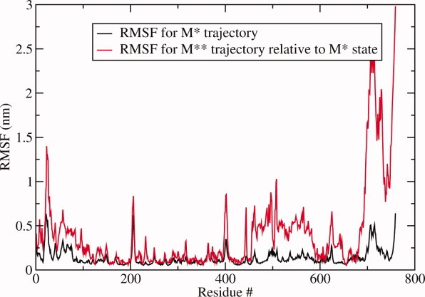
Root-mean-square fluctuations (RMSF) measured for C_α atoms. Black line: values obtained for the M* trajectory in explicit solvent with respect to the average structure after aligning all timeframes to M* conformation. Red line: the same quantity for M** trajectory computed relative to M* conformation after alignment along residues 100–400. Converter domain is seen as the region in which greatest divergence occurs. [Color figure can be viewed in the online issue, which is available at wileyonlinelibrary.com.]

Figure 8.

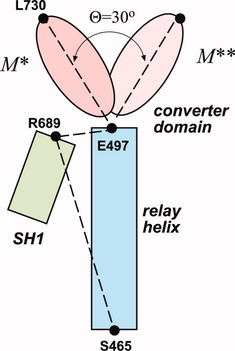
Cartoon defining the dihedral angle θ we use in this work to distinguish M* and M** states. The angle is formed by the line passing through C_α atoms of E497 and L730 with the plane formed by C_α atoms of E497, R689, and S465. [Color figure can be viewed in the online issue, which is available at wileyonlinelibrary.com.]

Two order parameters, RMSD over the 484–512 residues and angle θ, can be used to characterize structural transitions in myosin at both local and global levels. Figure 9 shows free energy estimate as a function of these two parameters obtained in implicit solvent simulations started from M* state. In the ATP-bound state, myosin should experience reversible M* to M** transitions, as demonstrated experimentally.² The locations of M* and M** states on the free energy map, shown by contours, suggest that such transition does not happen in our implicit solvent simulations. Observed changes in angle θare not accompanied by simultaneous restructuring in the relay helix and loop, as evidenced by high RMSD value in that region. We, therefore, conclude that our simulations do not show the recovery stroke transition in myosin. Similar conclusion is reached when the simulations are started from M** state (data not shown).

Figure 9.

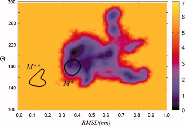
Estimate obtained from the implicit solvent M* simulations for free energy as a function of two order parameters: RMSD deviation from M** state over C_α of residues 484–512 and the angle θ characterizing the rotation state of the converter domain. Contours show the location of M** and M* states as seen in explicit solvent simulations. No global M* to M** transition is observed. Free energy is measured in units of kT, where k is the Boltzmann constant. [Color figure can be viewed in the online issue, which is available at wileyonlinelibrary.com.]

Discussion

Loose coupling between nucleotide binding site and force generation region in myosin

Our simulations offer new insights into the recovery stroke transition in myosin. It is believed that the recovery stroke is triggered by the SWII closure,⁹ initiating conformational changes that lead to the converter domain rotation. There are two interpretations of the communication mechanism between the nucleotide binding site and the force-generation region. First, based on minimal energy calculations, Fischer et al.⁹ argue that a definite path of intermediate steps exists between M* and M** states along which the transition takes place. In the early proposal,⁹ the R238–E459 salt bridge formation helps to close SWII, which in turn pulls on the N-terminal end of relay helix through the side chain of N475. As a result, the relay helix see-saws around the anchor point formed by F652–F481–F482 hydrophobic cluster. Since the relay helix has only limited range of movement in M* state, the continuing pull causes the hydrogen bonds to rupture between residues 486 and 487, creating a kink in the helix and leading to subsequent rotation of the converter domain. In later models,^8,10 the initial SWII closure remains the same but the converter rotation is caused by the piston-like displacement of SH1 helix, mediated by a wedge loop of residues 572–574. Although the microscopic details differ in these models, what they have in common is an ordered sequence of transitions among clearly defined intermediate states along which the reaction progresses. This mechanistic view has been questioned by the second group of proposals,^13,15–17 arguing against strong coupling between SWII and the force-generation domain. Evidence from enhanced sampling simulations^15,16 shows that SWII may remain closed while the rotation of the converter domain is not complete. The same is true for rotated converter while the SWII is open. Although there is a correlation between the states of two structural elements, it is not strong enough to warrant a mechanistic interpretation. Instead, the authors advance a statistical explanation based on “ensemble shifts,” according to which the rotated converter is statistically favored for closed SWII state, but not linked to it in a deterministic manner. The ensembles argument admits a significant role for the entropy in the transition,¹⁶ supported by a large entropy difference between M* and M** states observed experimentally.³

Our simulations support this second, statistical interpretation. Starting from the initial pre-recovery state M* we see that the closure of the SWII occurs early on in the process, consistent with it being the trigger of the transition.⁹ Despite the SWII closure, we do not see a concomitant rotation of the converter domain in our simulations, suggesting that it occurs later on and on a longer time scale. Our results are thus most consistent with the idea of the recovery stroke being a two-step process consisting of the SWII trigger and the converter rotation, which are separated by a time delay.¹³ The coupling between the two steps appears to be weak but its exact mechanism cannot be learned in our simulations.

Is SWII closure a single step reaction?

As it is observed in our simulations, all SWII closing events lead essentially to the same configuration of the nucleotide binding pocket, identical to that observed experimentally. The lack of structural variability suggests that the trigger step is a simple reaction devoid of any detectable intermediates. The simplicity implies that the one-dimensional representation of the reaction is reasonable, justifying earlier studies based on one order parameter.¹⁵ The possibility of 1D modeling raises the following question: what is the reaction coordinate of that reaction? An obvious choice is the distance between hydrogen bonding atoms G457:N and ATP:P_γ. But with only a handful of SWII closing events, it is not possible to judge the quality of this choice at the moment. With the implicit solvent model described in this work it should be possible to generate better statistics in the future to give more definitive answers. The outcome of such studies is the ability to model properly the early stage of the recovery stroke. This includes the ability to rationalize the effect of mutations on the trigger reaction.²⁶

SWII closure: related experimental data

SWII in closed and open structural states was observed experimentally with X-ray crystallography, when myosin is trapped with a nucleotide analog.^27–29 These data were in agreement with nucleotide chase experiments,^4,30–32 which show slower rate of ATP dissociation than ADP, indicating closed conformation of SWII when ATP is bound and open SWII conformation with bound ADP. According to atomic structures, closed and open structural state of SWII is accompanied with bent and straight relay helix accordingly, and initially it was proposed that closed SWII and bent relay helix are rigidly coupled in one myosin structural state (M**). These structural rearrangements were interpreted as a reason for myosin intrinsic fluorescence change, observed earlier in kinetic studies of skeletal myosin.³³ Indeed, the surface accessibility area of one of myosin tryptophans (W501) changes substantially during the M* → M** structural transformation. But myosin W501 single tryptophan mutant shows unexpected drop of intrinsic fluorescence at initial stage of myosin–ATP interaction, indicating that other tryptophans (there are five tryptophans total in the skeletal myosin head) play a role in the intrinsic fluorescence change. Skeletal myosin has two tryptophans close to the nucleotide binding site, and the attempt to detect nucleotide binding kinetics and possibly kinetics of structural rearrangement of SWII was made with single tryptophan myosin mutants, when tryptophan was engineered near nucleotide binding site (W113, W129, and W131).³⁴ Unfortunately, these tryptophans were insensitive to SWII closure upon myosin–ATP interaction. Studies of spin labeled nucleotide analogs, bound to myosin, showed immobilization of the spin label upon nucleotide binding, but it was concluded that spin labeled nucleotide was not sensitive to SWII structural state.³⁵ Studies of fluorescent (mant) nucleotide binding to myosin concluded that fluorescence change of mant nucleotide upon its binding to myosin reflects only binding event and not SWII closure.³² Temperature jump studies^2,6 showed that intrinsic fluorescence of myosin, trapped with a nucleotide analog, changes upon temperature jump, reflecting myosin conformation change with the same nucleotide analog bound. These were the first experimental results indicating that structures of the SWII and the relay helix are not rigidly coupled in M* and M** structural states of myosin. Recently, continuous wave EPR, pulsed EPR, and FRET studies of myosin, labeled with spin or fluorescent probes and trapped with nucleotide analogs, confirmed loose coupling between biochemical state of myosin (determined by bound nucleotide and as a result, closed or opened SWII) and the structural state of the force generating region.⁷ Our simulations confirm these recent experimental results, showing the absence of strict correspondence between the SWII and the relay helix structural states, and proposing that the SWII closure and structural changes in the force generating region are occurring at different times during the recovery stroke.

Methods and Models

Proteins in this work were modeled at the all-atom level using the AMBER99³⁶ force field modified by Hornak et al.³⁷ All simulations were performed by GROMACS4^38,39 package, with the implementation of the force field by Sorin and Pande.⁴⁰ The explicit solvent simulations were carried out using TIP3 water model.⁴¹ The generalized Born (GB)²⁰ implicit solvent model, as implemented by Onufriev et al.,²¹ was used in implicit solvent simulations. The dielectric constant ɛ was set to 80 in these simulations. The chemical bonds in water molecules were held constant by the SETTLE⁴² algorithm. The bonds involving hydrogen atoms in the protein were constrained according to the LINCS⁴³ algorithm.

In explicit solvent simulations, atomic structures, prepared as reported by Agafonov et al.,⁷ were placed in cubic boxes of 12–13 nm across containing 66,000–67,000 water molecules, and equilibrated with the heavy atoms constrained to their initial positions. Productive simulations were conducted at constant temperature using Nose-Hoover thermostat⁴⁴ with a 0.05 ps time constant. A single cut-off of 1 nm was used for the van der Waals interactions with the neighbor lists updated every 10 time steps. Smooth-particle mesh Ewald (PME)⁴⁵ was used to treat electrostatic interactions. In implicit solvent, a single cut-off of 1.2 nm was used for electrostatic and van der Waals forces. The time step was set 2 fs in all simulations.

A number of simulations were conducted at different temperatures and with different initial structures. The summary of all generated simulations, with the aggregate time of more than 2 μs, is shown in Table I.

Table I.

Summary of MD Simulations Performed in this Work

	Solvent	Simulations	Temperature
Initial conformation M*	Explicit	5 trajectories 10 ns each	300 K
	Implicit	10 trajectories 50 ns each	300 K, 350 K
Initial conformation M**	Explicit	5 trajectories 10 ns each	300K
	Implicit	10 trajectories 50 ns each	300 K, 350 K

Details of force-fields and solvent models are in the main text.

References

- 1.Lymn RW, Taylor EW. Mechanism of adenosine triphosphate hydrolysis by actomyosin. Biochemistry. 1971;10:4617–4624. doi: 10.1021/bi00801a004. [DOI] [PubMed] [Google Scholar]
- 2.Malnasi-Csizmadia A, Pearson DS, Kovacs M, Woolley RJ, Geeves MA, Bagshaw CR. Kinetic resolution of a conformational transition and the ATP hydrolysis step using relaxation methods with a Dictyostelium myosin II mutant containing a single tryptophan residue. Biochemistry. 2001;40:12727–12737. doi: 10.1021/bi010963q. [DOI] [PubMed] [Google Scholar]
- 3.Agafonov RV, Nesmelov YE, Titus MA, Thomas DD. Muscle and nonmuscle myosins probed by a spin label at equivalent sites in the force-generating domain. Proc Natl Acad Sci USA. 2008;105:13397–13402. doi: 10.1073/pnas.0801342105. [DOI] [PMC free article] [PubMed] [Google Scholar]
- 4.Gyimesi M, Kintses B, Bodor A, Perczel A, Fischer S, Bagshaw CR, Malnasi-Csizmadia A. The mechanism of the reverse recovery step, phosphate release, and actin activation of Dictyostelium myosin II. J Biol Chem. 2008;283:8153–8163. doi: 10.1074/jbc.M708863200. [DOI] [PubMed] [Google Scholar]
- 5.Sweeney HL, Houdusse A. Structural and functional insights into the myosin motor mechanism. Annu Rev Biophys. 2010;39:539–557. doi: 10.1146/annurev.biophys.050708.133751. [DOI] [PubMed] [Google Scholar]
- 6.Wray J, Urbanke C. A fluorescence temperature-jump study of conformational transitions in myosin subfragment 1. Biochem J. 2001;358:165–173. doi: 10.1042/0264-6021:3580165. [DOI] [PMC free article] [PubMed] [Google Scholar]
- 7.Agafonov RV, Negrashov IV, Tkachev YV, Blakely SE, Titus MA, Thomas DD, Nesmelov YE. Structural dynamics of the myosin relay helix by time-resolved EPR and FRET. Proc Natl Acad Sci USA. 2009;106:21625–21630. doi: 10.1073/pnas.0909757106. [DOI] [PMC free article] [PubMed] [Google Scholar]
- 8.Mesentean S, Koppole S, Smith JC, Fischer S. The principal motions involved in the coupling mechanism of the recovery stroke of the myosin motor. J Mol Biol. 2007;367:591–602. doi: 10.1016/j.jmb.2006.12.058. [DOI] [PubMed] [Google Scholar]
- 9.Fischer S, Windshugel B, Horak D, Holmes KC, Smith JC. Structural mechanism of the recovery stroke in the myosin molecular motor. Proc Natl Acad Sci USA. 2005;102:6873–6878. doi: 10.1073/pnas.0408784102. [DOI] [PMC free article] [PubMed] [Google Scholar]
- 10.Koppole S, Smith JC, Fischer S. The structural coupling between ATPase activation and recovery stroke in the myosin II motor. Structure. 2007;15:825–837. doi: 10.1016/j.str.2007.06.008. [DOI] [PubMed] [Google Scholar]
- 11.Koppole S, Smith JC, Fischer S. Simulations of the myosin II motor reveal a nucleotide-state sensing element that controls the recovery stroke. J Mol Biol. 2006;361:604–616. doi: 10.1016/j.jmb.2006.06.022. [DOI] [PubMed] [Google Scholar]
- 12.Yamanaka K, Okimoto N, Neya S, Hata M, Hoshino T. Behavior of water molecules in ATPase pocket of myosin. J Mol Struct-Theochem. 2006;758:97–105. [Google Scholar]
- 13.Elber R, West A. Atomically detailed simulation of the recovery stroke in myosin by Milestoning. Proc Natl Acad Sci USA. 2010;107:5001–5005. doi: 10.1073/pnas.0909636107. [DOI] [PMC free article] [PubMed] [Google Scholar]
- 14.Yang Y, Yu HB, Cui Q. Extensive conformational transitions are required to turn on ATP hydrolysis in myosin. J Mol Biol. 2008;381:1407–1420. doi: 10.1016/j.jmb.2008.06.071. [DOI] [PMC free article] [PubMed] [Google Scholar]
- 15.Yu HB, Ma L, Yang Y, Cui Q. Mechanochemical coupling in the myosin motor domain. I. Insights from equilibrium active-site simulations. Plos Comput Biol. 2007;3:199–213. doi: 10.1371/journal.pcbi.0030021. [DOI] [PMC free article] [PubMed] [Google Scholar]
- 16.Harris MJ, Woo HJ. Energetics of subdomain movements and fluorescence probe solvation environment change in ATP-bound myosin. Eur Biophys J. 2008;38:1–12. doi: 10.1007/s00249-008-0347-3. [DOI] [PubMed] [Google Scholar]
- 17.Woo HJ. Exploration of the conformational space of myosin recovery stroke via molecular dynamics. Biophys Chem. 2007;125:127–137. doi: 10.1016/j.bpc.2006.07.001. [DOI] [PubMed] [Google Scholar]
- 18.Nesmelov YE, Agafonov RV, Negrashov IV, Blakely SE, Titus MA, Thomas DD. Structural kinetics of myosin by transient time-resolved FRET. Proc Natl Acad Sci USA. 2011;108:1891–1896. doi: 10.1073/pnas.1012320108. [DOI] [PMC free article] [PubMed] [Google Scholar]
- 19.Feig M, Brooks CL. Recent advances in the development and application of implicit solvent models in biomolecule simulations. Curr Opin Struct Biol. 2004;14:217–224. doi: 10.1016/j.sbi.2004.03.009. [DOI] [PubMed] [Google Scholar]
- 20.Bashford D, Case DA. Generalized Born models of macromolecular solvation effects. Annu Rev Phys Chem. 2000;51:129–152. doi: 10.1146/annurev.physchem.51.1.129. [DOI] [PubMed] [Google Scholar]
- 21.Onufriev A, Bashford D, Case DA. Exploring protein native states and large-scale conformational changes with a modified generalized born model. Proteins-Struct Funct Bioinformatics. 2004;55:383–394. doi: 10.1002/prot.20033. [DOI] [PubMed] [Google Scholar]
- 22.Geeves MA, Holmes KC. Structural mechanism of muscle contraction. Annu Rev Biochem. 1999;68:687–728. doi: 10.1146/annurev.biochem.68.1.687. [DOI] [PubMed] [Google Scholar]
- 23.Sasaki N, Shimada T, Sutoh K. Mutational analysis of the switch II loop of Dictyostelium myosin II. J Biol Chem. 1998;273:20334–20340. doi: 10.1074/jbc.273.32.20334. [DOI] [PubMed] [Google Scholar]
- 24.Onishi H, Kojima S, Katoh K, Fujiwara K, Martinez HM, Morales MF. Functional transitions in myosformation of a critical salt-bridge and transmission of effect to the sensitive tryptophan. Proc Natl Acad Sci USA. 1998;95:6653–6658. doi: 10.1073/pnas.95.12.6653. [DOI] [PMC free article] [PubMed] [Google Scholar]
- 25.Furch M, Fujita-Becker S, Geeves MA, Holmes KC, Manstein DJ. Role of the salt-bridge between switch-1 and switch-2 of Dictyostelium myosin. J Mol Biol. 1999;290:797–809. doi: 10.1006/jmbi.1999.2921. [DOI] [PubMed] [Google Scholar]
- 26.Murphy CT, Rock RS, Spudich JA. A myosin II mutation uncouples ATPase activity from motility and shortens step size. Nat Cell Biol. 2001;3:311–315. doi: 10.1038/35060110. [DOI] [PubMed] [Google Scholar]
- 27.Gulick AM, Bauer CB, Thoden JB, Rayment I. X-ray structures of the MgADP, MgATPgammaS, and MgAMPPNP complexes of the Dictyostelium discoideum myosin motor domain. Biochemistry. 1997;36:11619–11628. doi: 10.1021/bi9712596. [DOI] [PubMed] [Google Scholar]
- 28.Fisher AJ, Smith CA, Thoden JB, Smith R, Sutoh K, Holden HM, Rayment I. X-ray structures of the myosin motor domain of Dictyostelium discoideum complexed with MgADP.BeFx and MgADP.AlF4. Biochemistry. 1995;34:8960–8972. doi: 10.1021/bi00028a004. [DOI] [PubMed] [Google Scholar]
- 29.Smith CA, Rayment I. X-ray structure of the magnesium(II) ADP vanadate complex of the Dictyostelium discoideum myosin motor domain to 1.9 A resolution. Biochemistry. 1996;35:5404–5417. doi: 10.1021/bi952633+. [DOI] [PubMed] [Google Scholar]
- 30.Phan BC, Cheung P, Stafford WF, Reisler E. Complexes of myosin subfragment-1 with adenosine diphosphate and phosphate analogs: probes of active site and protein conformation. Biophys Chem. 1996;59:341–349. doi: 10.1016/0301-4622(95)00127-1. [DOI] [PubMed] [Google Scholar]
- 31.Woodward SKA, Eccleston JF, Geeves MA. Kinetics of the interaction of 2′(3′)-O-(N-methylanthraniloyl)-ATP with myosin subfragment-1 and actomyosin subfragment-1—characterization of 2 Acto.S1.Adp Complexes. Biochemistry. 1991;30:422–430. doi: 10.1021/bi00216a017. [DOI] [PubMed] [Google Scholar]
- 32.Jahn W. The association of actin and myosin in the presence of gamma-amido-ATP proceeds mainly via a complex with myosin in the closed conformation. Biochemistry. 2007;46:9654–9664. doi: 10.1021/bi700318t. [DOI] [PubMed] [Google Scholar]
- 33.Johnson KA, Taylor EW. Intermediate states of subfragment-1 and actosubfragment-1 ATPase—re-evaluation of mechanism. Biochemistry. 1978;17:3432–3442. doi: 10.1021/bi00610a002. [DOI] [PubMed] [Google Scholar]
- 34.Kovacs M, Malnasi-Csizmadia A, Woolley RJ, Bagshaw CR. Analysis of nucleotide binding to Dictyostelium myosin II motor domains containing a single tryptophan near the active site. J Biol Chem. 2002;277:28459–28467. doi: 10.1074/jbc.M202180200. [DOI] [PubMed] [Google Scholar]
- 35.Naber N, Purcell TJ, Pate E, Cooke R. Dynamics of the nucleotide pocket of myosin measured by spin-labeled nucleotides. Biophys J. 2007;92:172–184. doi: 10.1529/biophysj.106.090035. [DOI] [PMC free article] [PubMed] [Google Scholar]
- 36.Wang JM, Cieplak P, Kollman PA. How well does a restrained electrostatic potential (RESP) model perform in calculating conformational energies of organic and biological molecules? J Comput Chem. 2000;21:1049–1074. [Google Scholar]
- 37.Hornak V, Abel R, Okur A, Strockbine B, Roitberg A, Simmerling C. Comparison of multiple amber force fields and development of improved protein backbone parameters. Proteins-Struct Funct Bioinformatics. 2006;65:712–725. doi: 10.1002/prot.21123. [DOI] [PMC free article] [PubMed] [Google Scholar]
- 38.van der Spoel D, Lindahl E, Hess B, Groenhof G, Mark AE, Berendsen HJC. GROMACS: fast, flexible, and free. J Comput Chem. 2005;26:1701–1718. doi: 10.1002/jcc.20291. [DOI] [PubMed] [Google Scholar]
- 39.Hess B, Kutzner C, van der Spoel D, Lindahl E. GROMACS 4: algorithms for highly efficient, load-balanced, and scalable molecular simulation. J Chem Theory Comput. 2008;4:435–447. doi: 10.1021/ct700301q. [DOI] [PubMed] [Google Scholar]
- 40.Sorin EJ, Pande VS. Exploring the helix-coil transition via all-atom equilibrium ensemble simulations. Biophys J. 2005;88:2472–2493. doi: 10.1529/biophysj.104.051938. [DOI] [PMC free article] [PubMed] [Google Scholar]
- 41.Jorgensen WL, Chandrasekhar J, Madura JD, Impey RW, Klein ML. Comparison of simple potential functions for simulating liquid water. J Chem Phys. 1983;79:926–935. [Google Scholar]
- 42.Miyamoto S, Kollman PA. SETTLE—an analytical version of the SHAKE and RATTLE algorithm for rigid water models. J Comput Chem. 1992;13:952–962. [Google Scholar]
- 43.Hess B, Bekker H, Berendsen HJC, Fraaije J. LINCS: a linear constraint solver for molecular simulations. J Comput Chem. 1997;18:1463–1472. [Google Scholar]
- 44.Nose S. Constant temperature molecular-dynamics methods. Prog Theor Phys Supp. 1991;103:1–46. [Google Scholar]
- 45.Essmann U, Perera L, Berkowitz ML, Darden T, Lee H, Pedersen LG. A smooth particle mesh Ewald method. J Chem Phys. 1995;103:8577–8593. [Google Scholar]