

Abstract
Quantification of exposure to traffic-related air pollutants near highways is hampered by incomplete knowledge of the scales of temporal variation of pollutant gradients. The goal of this study was to characterize short-term temporal variation of vehicular pollutant gradients within 200–400 m of a major highway (>150 000 vehicles/d). Monitoring was done near Interstate 93 in Somerville (Massachusetts) from 06:00 to 11:00 on 16 January 2008 using a mobile monitoring platform equipped with instruments that measured ultrafine and fine particles (6–1000 nm, particle number concentration (PNC)); particle-phase (>30 nm) , , and organic compounds; volatile organic compounds (VOCs); and CO2, NO, NO2, and O3. We observed rapid changes in pollutant gradients due to variations in highway traffic flow rate, wind speed, and surface boundary layer height. Before sunrise and peak traffic flow rates, downwind concentrations of particles, CO2, NO, and NO2 were highest within 100–250 m of the highway. After sunrise pollutant levels declined sharply (e.g., PNC and NO were more than halved) and the gradients became less pronounced as wind speed increased and the surface boundary layer rose allowing mixing with cleaner air aloft. The levels of aromatic VOCs and , and organic aerosols were generally low throughout the morning, and their spatial and temporal variations were less pronounced compared to PNC and NO. O3 levels increased throughout the morning due to mixing with O3-enriched air aloft and were generally lowest near the highway reflecting reaction with NO. There was little if any evolution in the size distribution of 6–225 nm particles with distance from the highway. These results suggest that to improve the accuracy of exposure estimates to near-highway pollutants, short-term (e.g., hourly) temporal variations in pollutant gradients must be measured to reflect changes in traffic patterns and local meteorology.
1 Introduction
Exposure to traffic-related air pollutants near highways is associated with adverse health effects including cardiopulmonary disease, asthma and reduced lung function (Brugge et al., 2007; Brunekreef et al., 1997; Gauderman et al., 2007; Hwang et al., 2005; McConnell et al., 2006; Nicolai et al., 2003; Van Vliet et al., 1997; Venn et al., 2001). These findings have motivated research to better understand the kinds and amounts of pollutants in the near-highway environment as well as the factors governing the temporal and spatial variations in pollutant concentrations. Much attention has been focused on ultrafine particles (UFP; diameter <100 nm) because they are more toxic per unit mass than particles with larger diameters (Dockery et al., 2007; Oberdörster et al., 1995). Studies have shown that concentrations of UFP as well as other primary vehicular emissions are elevated near highways but then decrease to background within several hundred meters primarily as a result of dilution (see Table 1). The factors that impact the magnitude and extent of these gradients include traffic conditions, temperature, relative humidity, topography, wind direction and speed, atmospheric stability, and mixing height.
Table 1. Summary of near-highway air pollution monitoring studies.
| Study | Location; highway | Distance from highway (m) | Time and season of measurement | Vehicles countsa | Pollutants measuredb |
|---|---|---|---|---|---|
| Zhu et al., 2002a | Los Angeles; I-710 | 17–300c | 10:00–16:00; summer, fall | 12 180 h−1 | UFP + FP (6–220 nm), BC, CO |
| Zhu et al., 2002b | Los Angeles; I-405 | 30–300c | 10:30–16:00; spring, summer | 13 900 h−1 | UFP + FP (6–220 nm), BC, CO |
| Zhu et al., 2004 | Los Angeles; I-405 + I-710 | 30–300 (I-405); 17–300 (I-710) | 10:00–16:00; winter | 200–270 min−1 (I-405); 280–230 min−1 (I-710) | UFP + FP (6–220 nm), BC, CO |
| Zhu et al., 2006 | Los Angeles; I-405 | 30–300 c | 23:30-05:00; winter | 20–70 min−1 | UFP + FP (6–220 nm), BC, CO |
| Hu et al., 2009 | Santa Monica, CA; I-10 | 30–2600c | 1–2 h before sunrise; winter, summer | 715 5-min−1 (winter); 340 5-min−1 (summer) | UFP, PM2.5, BC, CO, NOx |
| Hagler et al., 2009 | Raleigh, NC; I-440 | 20–300c | 00:00-23:59; summer | 125 000 d−1 | UFP + FP (20–1000 nm), PM2.5, PM10, BC, NOx, CO |
| Beckerman et al., 2008 | Toronto; Highway 401 | 0–1000 | Continuous and peak daily traffic periods; summer | ∼400 000 d−1 | UFP + FP (10–2500 nm), PM2.5, NOx, NO2, O3, BC, VOCs |
| Kittleson et al., 2004 | Minneapolis – St. Paul, MN; I-494, Hwy 62 | 0, 10, 700 | 13:00–17:00; fall | NR | UFP + FP (3–1000 nm), NOx, CO2, CO |
| Birmili et al., 2008 | Berlin; Highway A100 | 4, 80, 400 | Continuous; summer | 180 000 d−1 | UFP + FP (10–500 nm), |
| Hitchins et al., 2000 | Brisbane; Gateway Motorway + Wynnum Rd | 15–375c | NR | 2130–3400 h−1 | UFP, FP, + CP (15– 20000 nm), PM2.5 |
| Morawska et al., 1999 | Brisbane; Southeast Freeway | 10–210c | 06:00–17:15; spring, summer | NR | UFP + FP (16–626 nm) |
| Gramotnev + Ristovski, 2004 | Brisbane; Gateway Motorway + Wynnum Rd | 25–307 | 11:00–15:00; spring | 3700–5000 h−1 | UFP (4–163 nm) |
| Shi et al., 1999 | Birmingham, UK; A38, A441 | 2–100c | 12:02-18:24; winter | 30 000 d−1 | UFP, FP, + CP (10– 10 000 nm) |
| Roorda-Knape et al., 1998 | South Holland, Netherlands; A4, A12, A13, A20 | 15–330c | NR | 80 000–152 000 d−1 | PM2.5, PM10, BC, VOCs, NO2 |
| Kerminen et al., 2007 | Helsinki; Highway Itäväylä | 9, 65 | 00:00–12:00; winter | 300–400 h−1 (night); ∼3000 h−1 (morning) | UFP + FP (7–1020 nm) |
| Pirjola et al., 2006 | Helsinki; Highway Itäväylä | 0–140c | 07:00–09:30, 15:00–18:30; winter, summer | 40–70 min−1 (winter); 60–90 min−1 (summer) | UFP, FP, + CP (3– 10000 nm), NOx, CO |
| This study | Somerville, MA; I-93 | 27–395c | 06:00–11:00, winter | 6020–8770 h−1 | UFP + FP (6–1000 nm), NOx, CO2, O3, , , organics |
As reported in the article cited.
UFP = ultrafine particles (<100 nm); FP = fine particles (100–2500 nm); CP = coarse particles (>2500 nm); PM2.5 = mass of particles with aerodynamic diameter ≤2.5 μm; PM10 = mass of particles with aerodynamic diameter ≤10 μm; BC = black carbon;
Pollutant measurements were made along a transect(s) measured perpendicular to highway. NR = not reported.
The effects of wind direction and speed on near-highway pollutant gradients have been demonstrated in several studies. For example, Beckerman et al. (2008) reported that UFP and NO2 levels decreased to background within 300–500 m on the downwind side of Highway 401 in Toronto, while on the upwind side UFP and NO2 levels decreased to background within 100–200 m of the highway. Similar upwind-downwind differences have been reported for other highways by Hitchens et al. (2000), Zhu et al. (2002a, 2002b, 2006), and Hagler et al. (2009). Of these, the findings of Zhu et al. (2006) are particularly noteworthy. Zhu et al. showed that upwind-downwind UFP gradients near I-405 in Los Angeles were reversed following a 180-degree change in prevailing wind direction. Also, they showed that UFP levels varied inversely with wind speed: UFP levels decreased by a factor of 2.5 following a 2.4-fold increase in wind speed.
Atmospheric stability and mixing height also strongly influence pollution gradients near highways. Jänhall et al. (2006) showed that peak concentrations of UFP, CO, NO and NO2 measured during the morning rush hour at a fixed site in Göteborg, Sweden, were between 2- and 6-fold higher on days with surface temperature inversions compared to days without inversions. Furthermore, they found that once the surface boundary layer lifted by late morning and surface air layers were able to mix with those aloft, traffic-related pollutant concentrations decreased to the same levels observed on days without inversions. In a year-long study of polycyclic aromatic hydrocarbons (PAH) and other traffic-related pollutants in Quito, Ecuador, Brachtl et al. (2009) found that pollutant levels increased sharply after 05:00, peaked at around 06:00–07:00, and then decreased sharply thereafter despite the relative constancy of traffic flow. This pattern was attributed to near-daily surface temperature inversions that are most pronounced just before sunrise.
Two studies from the Los Angeles Basin further demonstrate the importance of atmospheric stability. Zhu et al. (2006) found that UFP concentrations at 30 m from I-405 were only 20% lower at night (22:30–04:00) than during the day despite a 75% decrease in nighttime traffic flow. This apparent discrepancy was attributed to a combination of higher vehicle speeds, lighter winds, decreased air temperature, and increased relative humidity during the nighttime. Hu et al. (2009) found that pre-sunrise UFP levels were elevated above background as far as 600-m upwind and 2600-m downwind from I-10 despite relatively low traffic flow. Also, pre-sunrise pollutant concentrations were much higher during the winter than summer. These observations were attributed to surface temperature inversions and low wind speeds that are characteristic of the LA Basin in pre-sunrise hours. Seasonal differences in pollutant concentrations may be due in part to differences in boundary layer heights. Hu et al. reported that temperature inversions occurred at a lower elevation in the atmosphere in winter compared to summer, and that this, combined with relatively low nighttime winds in winter, resulted in shallower surface mixed layers during winter monitoring.
Knowledge of the causes of variations in the magnitude and extent of traffic-related pollutant gradients near highways has relevance for minimizing exposure assessment errors in health effects studies. Because pollutant levels at a given location can vary significantly throughout the day, repeated measurements must be made to properly characterize this variation. With the exception of a few recent studies (e.g., Jänhall et al., 2006; Hu et al., 2009), relatively little work has been done to measure the rates of change of near highway air pollution gradients. Therefore, the objective of our study was to measure hourly variations in near-highway air pollutant gradients. We did this using a mobile monitoring platform equipped with rapid response instruments. The pollutants studied included ultrafine and fine particles, gas-phase volatile organic compounds, CO2, NO, NO2, O3, and particle-phase , , and organic compounds. The study was conducted on a weekday morning in winter to capture near-highway air pollutant gradients under heavy traffic conditions during the transition from relatively light pre-sunrise winds to stronger winds following sunrise.
2 Methods
2.1 Study area
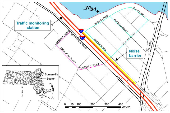
The study was performed near Interstate 93 (I-93) in the eastern part of Somerville, Massachusetts (Fig. 1). I-93 has four north-bound and four south-bound lanes, is 40-m-wide, and carries an average of ∼150 000 vehicles per day (MA Highway Dept, 2008). The highway is elevated 4.5–6m above street level in the study area and is filled underneath except at crossing points for local roads. The northbound lane is flanked on its east side by a 3-m-high concrete sound barrier. Sound barriers are of significance as they tend to impact pollution levels near highways (Baldauf et al., 2008). Massachusetts Route 38, a four-lane highway carrying ∼20 000 vehicles/day (MA Highway Dept., 2008), runs parallel to I-93 through the study area; Massachusetts Route 28, a six-lane highway that carries ∼50000 vehicles/day (MA Highway Dept., 2008), runs at a 60° angle to I-93 southeast of the study area (Fig. 1). Neither Routes 38 nor 28 are elevated above grade. The study area is bordered by the Mystic River to the north, Massachusetts Route 28 to the south and east, and Winter Hill (elevation=40 m) to the west. The area is relatively flat with the exception of a small hill (elevation=18 m) located near the intersection of Putnam Road and Temple Road. The study area is thickly settled with many single-and two-family houses and two- and three-story apartment buildings within 25–400 m of the highway. Other than highway and street traffic (particularly on the west side of I-93), the study area contains no other known significant sources of air pollution. Only one day of monitoring was performed. Our goal was to characterize a relatively typical weekday morning in winter when the combination of light pre-sunrise winds (<4 m/s), rush hour traffic, and cold-temperature combustion conditions would yield high concentrations of traffic-related air pollutants near the highway. 16 January 2008 met those requirements. Monitoring was done between 06:00 and 11:00, before, during, and after morning rush hour.
Fig. 1. Map of monitoring area.
2.2 Data collection
Real-time measurements of particle size distribution and particle number concentration (PNC), CO2, NO, NO2, O3, aromatic volatile organic compounds (AVOC; the sum of benzene, toluene, xylene isomers, ethyl benzene and C3-benzene isomers), and particle-bound nitrate, sulfate, and organics were made using the Aerodyne Research Inc. (ARI) mobile laboratory (AML) (Kolb et al., 2004). The AML is a walk-in panel truck equipped with a suite of air-monitoring instruments, a GPS receiver, computers, a power generator, batteries, and a video camera. NO2 was measured with a quantum cascade tunable infrared laser differential absorption spectrometer (QC-TILDAS; ARI, Billerica, MA) operating at 1606 cm−1. CO2 was measured with a non-dispersive infrared sensor (Model 6262, LI-COR, Lincoln, NB), NO was measured with a chemiluminescence analyzer (Model 42i, Thermo Fischer, Waltham, MA), O3 was measured with an ultra-violet absorption monitor (Model 205, 2B-Tech, Boulder, CO), and AVOCs were measured with a proton-transfer mass spectrometer (PTR-MS, Ionicon Analytik, Austria). Size distributions of airborne particles (6–225 nm) were measured using a scanning mobility particle sizer (SMPS; Model 3076, TSI, Shoreview, MN), and total particle number concentration (7–1000 nm) was measured using a condensation particle counter (CPC; Model 3022A, TSI).
An Aerodyne aerosol mass spectrometer (AMS) (Jayne et al., 2000; Canagaratna et al., 2007) with a C-ToF spectrometer (Drewnick et al., 2005) was used to measure chemical composition of size-resolved submicron particles. The AMS measures chemically-speciated mass loadings of aerosol particles in the 50–1000 nm size range. A collection efficiency of 0.5 (Canagaratna et al., 2007 and references therein) was used in the calculation of the reported mass concentrations. Contributions from inorganic species were identified according to the method published by Allan et al. (2004). Mass spectra were analyzed using positive matrix factorization (Lanz et al., 2007; Ulbrich et al., 2009).
The chemiluminescence sensor and the PTR-MS were both calibrated by successive dilution of air from cylinders containing concentration standards as described elsewhere (Wood et al., 2008; Rogers et al., 2006), leading to uncertainties of 10% for NO (2σ) and 25% for AVOC (1σ). The NO2 measurements were calibrated with a similarly diluted standard (NO2 produced via ozonolysis of 30 ppm NO in nitrogen) with an uncertainty (2σ) of 12%. The CO2 sensor response was checked with a two-point calibration at 0 and 400 ppm CO2 in air (Scott Specialty Gases) with an estimated uncertainty (2σ) of 5%. The manufacturer-stated uncertainty (2σ) of the O3 measurements was 2%.
The particle inlet manifold was made from stainless steel and copper tubing – to minimize particle loss due to electrostatic deposition – and equipped with a cyclone separator to remove coarse (>2.5 μm) particles. The gas inlet manifold was made from perfluoro-alkoxy Teflon™ tubing and contained a 0.45-μm Teflon filter. All instruments were operated at a frequency of 1 Hz with the exception of the SMPS and the AMS, which reported measurements every 110 and 15 s, respectively.
Continuous measurements were recorded throughout the monitoring period as the AML was repeatedly driven along roadways on either side of I-93 (Fig. 1). The wind blew primarily from the northwest throughout the monitoring period (Fig. 2); therefore, Memorial Road, Temple Street, and Mystic Avenue (Route 38) on the west side of I-93 were selected as the upwind transects, while Shore Drive, Bailey Road, Putnam Road, and Temple Road on the east side of I-93 were used as the downwind transects (Fig. 1). The AML was driven as slowly as traffic allowed (2.2–11 m/s) to capture local-scale changes in pollutant levels. It took 45– 60 min to cover all of the transects depending on traffic. The downwind transects were monitored 5 times and the upwind transects 3 times throughout the morning. There is a gap in the data from 08:07 and 09:22 when the AML was monitoring in a different part of the neighborhood (data not shown). Wind speed, wind direction, and air temperature data were recorded at the Hormel Stadium light tower (height=40 m) in the city of Medford, ∼0.5 km north of the study site. Hourly vehicle counts for I-93 station 8449 were provided by the Massachusetts Highway Department.
Fig. 2.
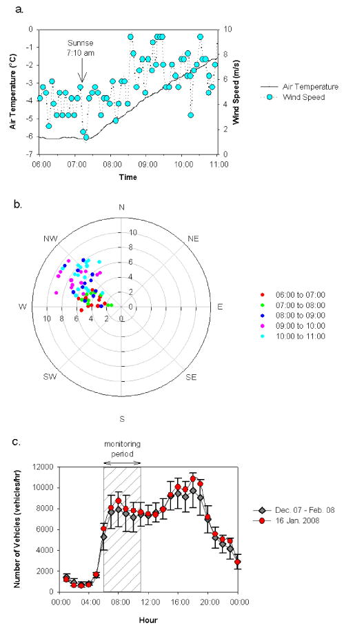
Weather and traffic data from 16 January 2008. (a) Time-series of air temperature and wind speed; (b) 5-min average of wind speed and wind direction data collected between 06:00 and 11:00 at the Hormel Stadium light tower in Medford, ∼0.5 km from monitoring area; (c) time-series of traffic flow on I-93 in both the north and south lanes measured at Somerville-Medford line. Weekday hourly average traffic volume (± one SD) on I-93 during the winter of 2008 are also shown.
2.3 Data reduction
Unusually high concentrations of AVOC – defined as values higher than the upper quartile + 1.5-times the interquartile range based on box plot analysis (Devore, 2004) – were considered indicative of self-sampling or encounters with nearby vehicle exhaust plumes; therefore, they (<10% of the total) were removed from the dataset along with corresponding measurements from the other instruments. Self-sampling episodes and plumes from nearby vehicles were confirmed by the on-board video record and/or the written log. GPS data were analyzed using ArcGIS 9.2 (ESRI, Redlands, CA). Data from the SMPS was adjusted following a laboratory calibration of the instrument after sampling. Due to the frequency of data acquisition by the monitors and the slow speed at which the AML was traveling, several measurements of each pollutant (with the exception of SMPS and AMS measurements) were taken at approximately the same location during a given run. These measurements were averaged prior to data analysis. For example, the “08:07” run took place from 08:06 to 08:10 as the AML was driven from 395 to 35 m from the highway. Each data point for this run represents 10 (±5) 1-s measurements that were averaged together. Also, for times when the AML was not moving (e.g., when it was at a traffic light or had stopped to measure wind speed and direction), data are presented as the mean and standard deviation of the stationary measurements. The averaged data were not significantly different than non-averaged data according to the Wilcoxon Rank Sum Test with p < 0.05.
3 Results and discussion
3.1 Meteorological and traffic conditions
On 16 January 2008 it was partly cloudy from 06:00 to 09:00 and mostly clear thereafter. There was no precipitation during the monitoring period (06:00–11:00); the 24-h mean barometric pressure and relative humidity were 30.20 inches of Hg and 53%, respectively (http://www.wunderground.com, accessed: 29 June 2008). The air temperature was relatively constant (−6.1 °C) between the start of monitoring and sunrise, and rose steadily thereafter to −1.7 °C at 11:00 when monitoring ended (Fig. 2a). The wind was very light (2–5 m/s) before sunrise, and then increased after sunrise to 5–9 m/s by 11:00. The wind direction (WNW) was relatively constant over the 5-h monitoring period (Fig. 2b). These wind conditions are fairly typical for winter (December-February) in the Boston area. In the winter of 2008, the average wind speed one hour before sunrise in our study area was 3.6–5.4 m/s (gentle breeze) 31% of the time and <6.2m/s (light wind) 82% of the time. On 16 January 2008 the average wind speed in our study area for the hour preceding sunrise was ∼4 m/s. The predominant wintertime wind direction in the Boston area is northwesterly, which it was on 16 January 2008.
Traffic on I-93 changed modestly over the monitoring period as shown in Fig. 2c. The traffic flow rate was about 6000 (vehicles/h) at the start of monitoring at 06:00, peaked at 8800 vehicles/h at 08:00, and decreased gradually to 7800 vehicles/h by 11:00. These rates are typical of wintertime, weekday conditions in our study area (Fig. 2c). The fleet composition and average vehicle speed were not measured.
3.2 Spatial and temporal variation of CPC and SMPS measurements
Changes in highway traffic flow rate, wind speed, and surface boundary layer height greatly impacted pollutant gradients near I-93. Particle number concentrations (PNC) were highest early in the morning but then decreased rapidly after sunrise as the surface boundary layer lifted between 08:07 and 09:20 (see Sect. 3.3) and wind speed increased (Fig. 3). Between 06:00 and 08:00 downwind PNC was highest (7×10⁴−9×10⁴ particles/cm3) at 34 m from I-93, the nearest point at which measurements were made, but decreased ∼2-fold within 100–250 m from the highway. Beyond 250 m downwind, PNC values were relatively constant at ∼3×10⁴ particles/cm3. After 09:00 the highest downwind PNC values again occurred nearest to I-93, but were 2-3-fold lower (∼3×10⁴ particles/cm3) compared to measurements made between 06:00 and 08:00. Upwind of I-93 the highest PNC values, measured nearest to the highway (40 m), were about 40% lower than the highest downwind concentrations, and dropped off sharply at 60–70 m. Beyond this distance, the profiles were relatively flat, indicative of well-mixed conditions. It is likely that the PNC spikes immediately upwind of the highway were caused by traffic on Rt. 38. As was observed in the downwind profiles, PNC levels in the upwind profiles were also generally higher early in the morning (06:37) compared to later in the morning (08:15 and 09:47). Our observations are in agreement with those of Hu et al. (2009) who found that above-background UFP levels extended much further from highway I-10 in LA (both upwind and downwind) before sunrise compared to after sunrise.
Fig. 3.
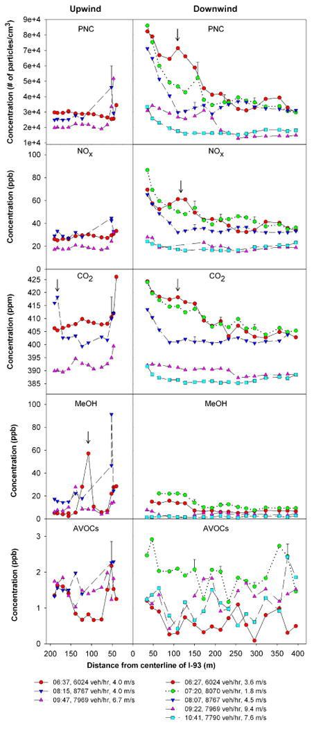
Spatial and temporal variation of particle number concentration (7–1000 nm), NOx, CO2, methanol (MeOH), and aromatic VOCs (AVOC) along transects perpendicular to I-93. Legend shows vehicles per hour on I-93 (both directions) and average hourly wind speed. Pollutant spikes indicated with arrows likely represent the plumes from vehicles passing nearby the AML; spikes immediately upwind of the highway were likely due to traffic on Rt. 38. Error bars (one SD) are shown at locations where the AML stopped briefly and multiple measurements were made.
We did not observe significant particle evolution with distance from the highway. The nearly linear relationship between PNC and CO2 (Fig. 4) suggests that PNC attenuation with distance was largely due to dilution. The slight convex curvature in the 06:27 and 07:20 data suggests some net particle formation (i.e., from nucleation and condensation into the >7-nm window of the CPC), which would be expected given the cold air temperature (−6.1–−1.7 °C), but the overall trend of these two plots is linear (R2 was >0.91 for both datasets), indicating that if evolution was occurring it was indistinguishable from noise in the dataset. This is consistent with Zhang et al. (2004) who compared the effects of particle dynamics (i.e., condensation and evaporation) and dilution on PNC near highways in LA and found that the effects of particle dynamics were generally much lower in winter than summer.
Fig. 4.
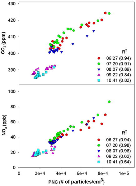
Relationship between CO2 and PNC and between NOx and PNC measured downwind of I-93 throughout the morning on 16 January 2008. Correlation coefficients (R2) are shown in the legends.
Particles <50 nm in diameter dominated the particle size distribution measurements throughout the morning; nearly 80% of particles counted in the 6–225 nm size range were <50nm (Fig. 5). Between 06:00 and 09:00 there were roughly equal number concentrations of particles in the 6–25 and 25–50 nm size ranges at each distance from I-93; however, after 09:00 there was an apparent shift toward relatively more particles occurring in the smallest size range. The relative number concentrations of >50 nm particles did not substantially change either with distance from the highway – which is consistent with other near-highway studies (Zhu et al., 2006; Hu et al., 2009) – or with time.
Fig. 5.
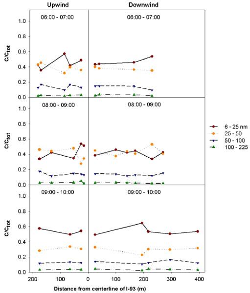
Spatial and temporal variation of particle size distribution along upwind and downwind transects perpendicular to I-93.
3.3 Spatial and temporal variation of gaseous pollutant measurements
Profiles of CO2 and NOx measured downwind of I-93 showed the same general spatial and temporal differences as were observed for PNC (Fig. 3). Between 06:00 and 08:00, CO2 and NOx were highest near I-93 and then decreased to background within 200–300 m downwind of the highway. After 09:00 near-highway concentrations were much lower compared to earlier times and the profiles were generally much flatter. Spatial and temporal variations in CO2 and NOx levels upwind of the highway were generally consistent with upwind variations in UFP Figure 4 shows the relationships between CO2 and PNC and between NOx and PNC downwind of I-93. As expected, the early morning correlations are much stronger – as indicated by higher R2 values – compared to later in the morning when mixing is greater.
O3 levels were nearly three-fold higher (>25ppb) after 09:00 compared to pre-sunrise levels (<10ppb), both upwind and downwind of the highway (Fig. 6). This strongly suggests that mixing with air from aloft was the dominant source of O3. Overlying air layers generally contain low levels of PNC, CO2 and NOx, so concentrations of these pollutants are expected to decrease at ground level after the surface boundary layer mixes. However, the opposite is true for O3: air layers aloft generally contain elevated levels of O3 (Trainer et al., 1987); thus, O3 levels were expected to increase at ground level after sunrise. The relatively low O3 levels measured near the highway – particularly in the 06:27, 07:20, and 08:07 downwind profiles – are likely attributable to reaction of O3 with NO. NO2 photolysis, which regenerates O3, was too slow to overcome O3 losses (Pinto et al., 2007). The post-sunrise increase in O3 is likely due to the breakup of the stable boundary layer, which is caused by nocturnal surface temperature inversions. Vertical temperature data for Boston was not readily available; however, based on data from the Massachusetts Department of Environmental Protection's vertical temperature profiler in Stowe, MA, located about 40 km to the west of our study area, early-morning surface inversions were present on about ∼20% of days from 21 December 2007 to 21 March 2008 (http://madis-data.noaa.gov/cap/profiler.jsp?options=full).
Fig. 6.
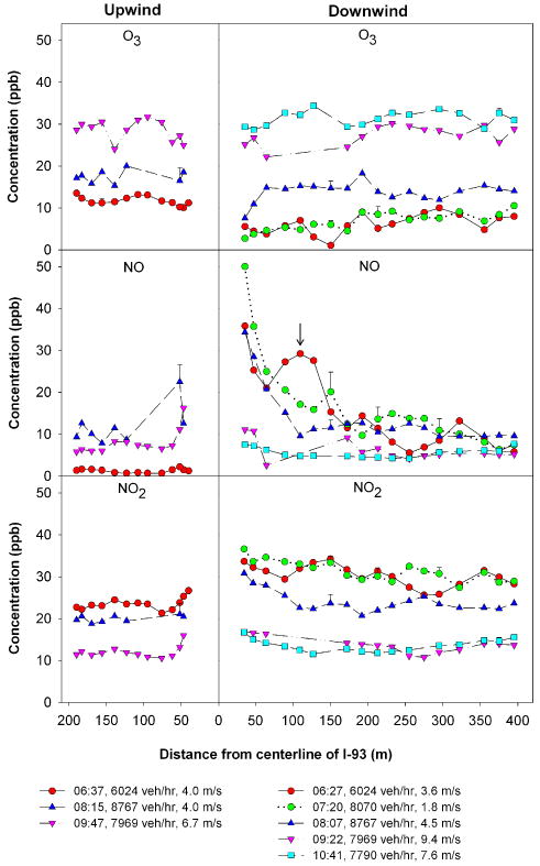
Spatial and temporal variation of O3, NO, and NO2 along transects perpendicular to I-93. Legend shows vehicles per hour on I-93 (both directions) and average hourly wind speed. Error bars (one SD) are shown at locations where the AML stopped briefly and multiple measurements were made. Spike in 06:27 NO profile (indicated with arrow) likely represents the plume from a vehicle passing nearby the AML; spikes immediately upwind of the highway were likely due to traffic on Rt. 38.
The downwind profiles for methanol show similar spatial and temporal variations to those exhibited by the other vehicle exhaust components (Fig. 3). Methanol concentrations downwind of I-93 were highest early in the morning when the winds were the lightest. Methanol is present in both vehicle exhaust and is a major component in windshield wiper fluid (Rogers et al., 2006). These emissions rapidly mix in ambient air and appear as a single source downwind from vehicles. The presence of methanol in windshield wiper fluids makes the methanol measurements sensitive and highly variable due to the presence of vehicles in the direct vicinity of the AML. The interference from local traffic is evident in Fig. 3 by the large spikes in the upwind profile.
The AVOC concentrations (the sum of the signals from benzene, toluene, xylene isomers, ethyl benzene and C3-benzene isomers) remained relatively constant throughout the morning and exhibit only weak spatial and temporal variations (Fig. 3). The high temporal response (100 ms dwell per mass) limited the precision of these measurements. Similar to the methanol, highest downwind AVOC concentrations were observed when winds were lightest. The AVOC concentrations are generally consistent with previous measurements made in the Boston area by Baker et al. (2008), which suggest an ambient AVOC concentration of 0.4 ppb with an enrichment of 4 ppt AVOC/ppb excess CO. Our measurements indicate that CO levels were enhanced by ∼200 ppb above background (results not shown), suggesting an AVOC concentration of ∼1.2 ppb, which is in good agreement with that shown in Fig. 3.
3.4 Spatial and temporal variation of particle composition measurements
Nitrate and sulfate aerosol concentrations (Fig. 7) were relatively low (<1 μg/m3) throughout the morning, and the profiles showed little spatial variation with distance from the highway. This was expected because vehicles are not significant direct emitters of nitrate aerosol, and the mandated use of ultra low sulfur diesel fuel (maximum sulfur content 15 ppm) leads to very low emissions of aerosol sulfate. The overall decrease in the levels of sulfate aerosol throughout the morning is attributable to the increase in surface boundary layer height. The increase in nitrate levels over the same period – except for the 10:41 downwind profile – likely reflects photooxidation of background NOx. Because the time scale for photooxidation of NOx to nitrate is relatively long compared to downwind transport (Sander et al., 2006), it is likely that photooxidation of freshly-emitted NOx from I-93 does not explain the increase in nitrate aerosol levels. Although the AMS is not sensitive to <30 nm particles and it is thus likely that our nitrate and sulfate aerosol concentration measurements underestimated the total, we do not believe this significantly impacts our conclusions.
Fig. 7.
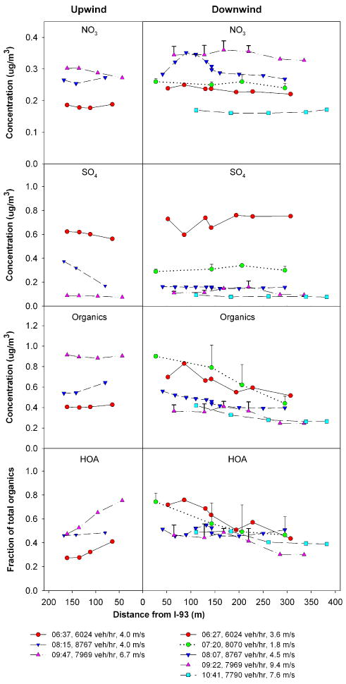
Spatial and temporal variation of , , organic aerosol and fraction hydrocarbon-like organic aerosol (HOA) along transects perpendicular to I-93. Legend shows vehicles per hour on I-93 (both directions) and average hourly wind speed. Error bars (one SD) are shown at locations where the AML stopped briefly and multiple measurements were made. The spike in the 07:20 and 09:47 organic aerosol profiles likely represent the plumes from vehicles passing nearby the AML.
The concentrations of organic aerosol were relatively low (<1.4 μg/m3) throughout the morning (Fig. 7). The downwind profiles <100 m from the highway showed the expected temporal variation, similar to that observed with PNC and NO (Fig. 3). At >100 m upwind there appeared to be local contributions of organic aerosol, particularly in the 08:15 and 09:47 profiles. Concentration differences between the 06:27-downwind and 06:37-upwind profiles are likely explained by high amounts of fresh highway emissions in the downwind profile. As in other urban areas (e.g., Zhang et al., 2007), two dominant organic components – hydrocarbon-like organic aerosol (HOA) and oxidized organic aerosol (OOA; approximated as the difference between the total organic aerosol mass and HOA mass) – accounted for 98% of the observed organic aerosol mass. The HOA component generally correlates well with tracers of vehicle emission (i.e., BC, CO, NOx) indicating it has a dominant contribution from fresh vehicle emissions; the oxidized nature of the OOA component reflects photochemically-aged urban aerosol (Cangaratna et al., 2007; Zhang et al., 2007).
3.5 Significance
The results of this study have significance for near-highway air pollution characterization and exposure assessment. The results show that pollutant levels change rapidly as a function of atmospheric mixing conditions and chemical reactions over short distances near highways. We observed that the levels of primary pollutants (UFP and NOx) were highest under light winds during pre-sunrise hours, and that following sunrise pollutant levels decreased rapidly both near the highway and downwind as the mixing height rose and wind speeds increased (Fig. 8). We also observed that the levels of reactive pollutants, such as O3 and NO, change rapidly over short distances in the near highway zone (Fig. 6). These rapid temporal and fine-grain spatial changes in pollutant levels highlight the need for rapid-response instruments housed in mobile monitoring platforms to characterize near-highway air pollution gradients.
Fig. 8.
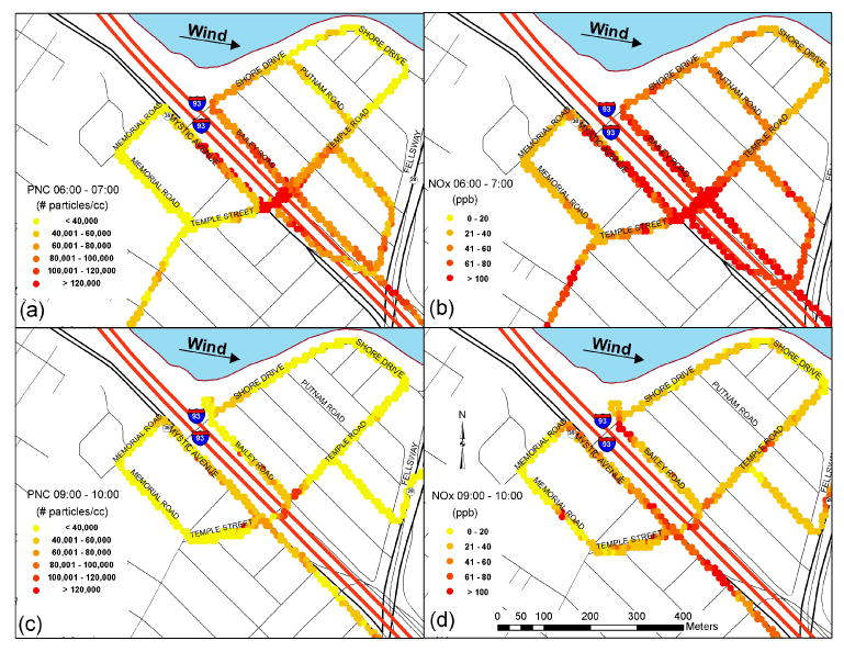
Spatial distribution of particle number concentration (7–1000 nm) (a and c) and NOx concentration (b and d) measured between 06:00–07:00 and between 09:00–10:00.
The high variability of near-highway pollution levels – particularly UFP – poses a challenge for exposure assessment. Assignment of air pollution exposure generally involves some degree of exposure misclassification; however, for UFP this problem is expected to be elevated compared to pollutants that demonstrate less geographic variation (e.g., PM2.5 and black carbon). This may partly explain the paucity of epidemiologic studies of UFP. Indeed, most studies of human health effects and PM have focused on PM2.5, PM10, black carbon or elemental carbon (see reviews in Hoek et al., 2009; Knol et al., 2009). These studies typically assign annual average exposure at residential addresses using measured levels at nearby fixed monitors or interpolation between multiple fixed monitors. For PM2.5, which varies relatively gradually across time and space, the error in exposure assessment introduced by movement of people (e.g., from their homes to where they work or go to school), results in only a limited amount of exposure misclassification. However, for pollutants like UFP that vary more substantially, the error is expected to be larger, perhaps large enough to compromise tests of association with health if exposure assessment approaches similar to PM2.5 studies are applied. This suggests that knowledge of short-term temporal and fine-grain spatial resolution of UFP is necessary in studies testing associations between UFP exposure and health outcomes. Further, high resolution pollutant data will need to be weighted by time-activity information in order to assign reasonably accurate exposures to individuals. Given our results here and those of others (e.g., studies cited in Table 1), geographic scaling on the order of tens of meters and time resolution on the order of hourly are needed to capture the rapid changes in near-highway pollutant levels with distance. Also, because meteorological and highway traffic conditions change on multiple time scales, it is necessary to perform monitoring throughout the day on different days and in different seasons to characterize the full range of variability and thereby allow more complete exposure assessments.
Acknowledgments
Traffic data was provided by the Massachusetts Highway Department. Funding for this work was provided by the Mystic View Task Force, Aerodyne Research, Inc. IR&D, and NIH grant ES015462.
References
- Allan JD, Coe H, Bower KN, Alfarra MR, Delia AE, Jimenez JL, Middlebrook AM, Drewnick F, Onasch TB, Canagaratna MR, Jayne JT, Worsnop DR. Extraction of Chemically Resolved Mass Spectra from Aerodyne Aerosol Mass Spectrometer Data. J Aerosol Sci Technol. 2004;35:909–922. [Google Scholar]
- Baker AK, Beyersdorf AJ, Doezema LA, Katzenstein A, Meinardi S, Simpson IJ, Blake DR, Rowland FS. Measurement of nonmethane hydrocarbons in 28 United States cities. Atmos Environ. 2008;42:170–182. [Google Scholar]
- Baldauf R, Thoma E, Khlystov A, Isakov V, Bowker G, Long T, Snow R. Impacts of noise barriers on near-road air quality. Atmos Environ. 2008;42:7502–7507. [Google Scholar]
- Beckerman B, Jerrett M, Brook JR, Verma DK, Arain MA, Finkelstein MM. Correlation of nitrogen dioxide with other traffic pollutants near a major expressway. Atmos Environ. 2008;34:51–59. [Google Scholar]
- Birmili W, Alaviippola B, Hinneburg D, Knoth O, Tuch T, Borken-Kleefeld J, Schacht A. Dispersion of traffic-related exhaust particles near the Berlin urban motorway – estimation of fleet emission factors. Atmos Chem Phys. 2009;9:2355–2374. doi: 10.5194/acp-9-2355-2009. [DOI] [Google Scholar]
- Brachtl MV, Durant JL, Paez C, Sempertegui F, Ovieda J, Naumova E, Griffiths J. Spatial and temporal variations and mobile source emissions of polycyclic aromatic hydrocarbons in Quito, Ecuador. Environ Pollut. 2009;157:528–536. doi: 10.1016/j.envpol.2008.09.041. [DOI] [PMC free article] [PubMed] [Google Scholar]
- Brugge D, Durant JL, Rioux C. Near highway exposure to motor vehicle pollutants: Emerging evidence of cardiac and pulmonary health risks. Environ Health. 2007;6(23) doi: 10.1186/1476-069X-6-23. available at: http://www.ehjournal.net/content/6/1/23. [DOI] [PMC free article] [PubMed]
- Brunekreef B, Janssen NA, de Hartog J, Harssema H, Knape M, vanVliet P. Air pollution from truck traffic and lung function in children living near motorways. Epidemiology. 1997;8:298–303. doi: 10.1097/00001648-199705000-00012. [DOI] [PubMed] [Google Scholar]
- Canagaratna MR, Jayne JT, Jimenez JL, Allan JD, Alfarra MR, Zhang Q, Onasch TB, Drewnick F, Coe H, Middlebrook A, Delia A, Williams LR, Trimborn AM, Northway MJ, DeCarlo PF, Kolb CE, Davidovits P, Worsnop DR. Chemical and Microphysical Characterization of Ambient Aerosols with the Aerodyne Aerosol Mass Spectrometer. Mass Spectrom Rev. 2007;26:185–222. doi: 10.1002/mas.20115. [DOI] [PubMed] [Google Scholar]
- Devore JL. Probability and Statistics for Engineering and the Sciences. 6th. Thomson Learning, Inc.; Belmont, CA: 2004. [Google Scholar]
- Dockery DW, Stone PH. Cardiovascular risks from fine particulate air pollution. New Engl J Med. 2007;356:511–513. doi: 10.1056/NEJMe068274. [DOI] [PubMed] [Google Scholar]
- Drewnick F, Hings SS, DeCarlo PF, Jayne JT, Gonin M, Fuhrer K, Weimer S, Jimenez JL, Demerjian KL, Borrmann S, Worsnop DR. A new Time-of-Flight Aerosol Mass Spectrometer (ToF-AMS) – Instrument Description and First Field Deployment. Aerosol Sci Technol. 2005;39:637–658. [Google Scholar]
- Gauderman WJ, Vora H, McConnell R, Berhane K, Gilliland F, Thomas D, Lurmann F, Avol E, Kunzli N, Jarrett M, Peters J. Effect of exposure to traffic on lung development from 10 to 18 years of age: A cohort study. Lancet. 2007;369:571–577. doi: 10.1016/S0140-6736(07)60037-3. [DOI] [PubMed] [Google Scholar]
- Gramotnev G, Ristovski Z. Experimental investigation of ultra-fine particle size distribution near a busy road. Atmos Environ. 2004;38:1767–1776. [Google Scholar]
- Hagler GSW, Baldauf RW, Thoma ED, Long TR, Snow RF, Kinsey JS, Oudejans L, Gullett BK. Ultra-fine particles near a major roadway in Raleigh, North Carolina: Downwind attenuation and correlation with traffic-related pollutants. Atmos Environ. 2009;43:1229–1234. [Google Scholar]
- Hitchins J, Morawska L, Wolff R, Gilbert D. Concentrations of submicrometre particles from vehicle emissions near a major road. Atmos Environ. 2000;34:51–59. [Google Scholar]
- Hoek G, Boogaard H, Knol A, de Hartog J, Slottje P, Ayres JG, Borm P, Brunekreef B, Donaldson K, Forastiere F, Holgate S, Kreyling WG, Nemery B, Pekkanen J, Stone V, Wichmann HE, van der Sluijs J. Concentration response functions for ultrafine particles and all-cause mortality and hospital admissions: results of a European expert panel elicitation. Environ Sci Technol. 2010;44:476–482. doi: 10.1021/es9021393. [DOI] [PubMed] [Google Scholar]
- Hu S, Fruin S, Kozawa K, Mara S, Paulson SE, Winer AM. A wide area of air pollutant impact downwind of a freeway during pre-sunrise hours. Atmos Environ. 2009;43:2541–2549. doi: 10.1016/j.atmosenv.2009.02.033. [DOI] [PMC free article] [PubMed] [Google Scholar]
- Hwang BF, Lee YL, Lin YC, Jaakkola JJ, Guo YL. Traffic related air pollution as a determinant of asthma among Taiwanese school children. Thorax. 2005;60:467–473. doi: 10.1136/thx.2004.033977. [DOI] [PMC free article] [PubMed] [Google Scholar]
- Janhäll S, Olofson KFG, Andersson PU, Pettersson JBC, Hallquist M. Evolution of the urban aerosol during winter temperature inversion episodes. Atmos Environ. 2006;40:5355–5366. [Google Scholar]
- Jayne JT, Leard DC, Zhang X, Davidovits P, Smith KA, Kolb CE, Worsnop DR. Development of an Aerosol Mass Spectrometer for Size and Composition. Analysis of Submicron Particles. Aerosol Sci Technol. 2000;33:49–70. [Google Scholar]
- Kerminen VM, Pakkanen TA, Mäkelä T, Hillamo RE, Sillanpää M, Rönkkö T, Virtanen A, Keskinen J, Pirjola L, Hussein T, Hämeri K. Development of particle number size distribution near a major road in Helsinki during an episodic inversion situation. Atmos Environ. 2000;41:1759–1767. [Google Scholar]
- Kittelson DB, Watts WF, Johnson JP. Nanoparticle emissions on Minnesota highways. Atmos Environ. 2004;38:9–19. [Google Scholar]
- Knol AB, de Hartog JJ, Boogaard H, Slottje P, van der Sluijs JP, Lebret E, Cassee FR, Wardekker JA, Ayres JG, Borm PJ, Brunekreef B, Donaldson K, Forastiere F, Holgate ST, Kreyling WG, Nemery B, Pekkanen J, Stone V, Wichmann HE, Hoek G. Expert elicitation on ultrafine particles: likelihood of health effects and causal pathways. Particle Fibre Toxicol. 2009;6(19):1. doi: 10.1186/1743-8977-6-19. available at: http://www.particleandfibretoxicology.com/content/6/1/19. [DOI] [PMC free article] [PubMed]
- Kolb C, Herndon S, McManus JB, Shorter J, Zahniser M, Nelson D, Jayne J, Canagaratna M, Worsnop D. Mobile Laboratory with Rapid Response Instruments for Real-Time Measurements of Urban and Regional Trace Gas and Particulate Distribution and Emission Source Characteristics. Environ Sci Technol. 2004;38:5694–5703. doi: 10.1021/es030718p. [DOI] [PubMed] [Google Scholar]
- Lanz VA, Alfarra MR, Baltensperger U, Buchmann B, Hueglin C, Prévôt ASH. Source apportionment of submicron organic aerosols at an urban site by factor analytical modelling of aerosol mass spectra. Atmos Chem Phys. 2007;7:1503–1522. doi: 10.5194/acp-7-1503-2007. [DOI] [Google Scholar]
- McConnell R, Berhane K, Yao L, Jerrett M, Lurmann F, Gilliland F, Kunzli N, Gauderman J, Avol E, Thomas D, Peters J. Traffic susceptibility, and childhood asthma. Environ Health Perspect. 2006;114:766–772. doi: 10.1289/ehp.8594. [DOI] [PMC free article] [PubMed] [Google Scholar]
- Morawska L, Thomas S, Gilbert D, Greenaway C, Rijnders E. A study of the horizontal and vertical profile of submicrometer particles in relation to a busy road. Atmos Environ. 1999;33:1261–1274. [Google Scholar]
- Nicolai T, Carr D, Weiland SK, Duhme H, von Ehrenstein O, Wagner C, von Mutius E. Urban traffic and pollutant exposure related to respiratory outcomes and atopy in a large sample of children. Eur Respir J. 2003;21:956–963. doi: 10.1183/09031936.03.00041103a. [DOI] [PubMed] [Google Scholar]
- Oberdorster G, Gelein RM, Ferin J, Weiss B. Association of particulate air pollution and acute mortality: Involvement of ultrafine particles? Inhal Toxicol. 1995;7:111–124. doi: 10.3109/08958379509014275. [DOI] [PubMed] [Google Scholar]
- Pirjola L, Paasonen P, Pfeiffer D, Hussein T, Hämeri K, Koskentalo T, Virtanen A, Rönkkö T, Keskinen J, Pakkanen TA, Hillamo RE. Dispersion of particles and trace gases nearby a city highway: Mobile laboratory measurements in Finland. Atmos Environ. 2006;40:867–879. [Google Scholar]
- Pinto JP, Rizzo M, McCluney L, Fitz-Simons T. Characterization of surface ozone concentrations in the United States. Extended Abstracts, Ninth Conference on Atmospheric Chemistry, American Meteorological Society, P2.6, 1.7; San Antonio, Texas, USA. 2007. [Google Scholar]
- Rogers TM, Grimsrud EP, Herndon SC, Jayne JT, Kolb CE, Allwine E, Westberg H, Lamb BK, Zavala M, Molina LT, Molina MJ, Knighton WB. On-road measurements of volatile organic compounds in the Mexico City metropolitan area using proton transfer reaction mass spectrometry. Int J Mass Spectrom. 2006;252:26–37. [Google Scholar]
- Roorda-Knape MC, Janssen NAH, De Hartog JJ, Van Vliet PHN, Harssema H, Brunekreef B. Air pollution from traffic in city districts near major motorways. Atmos Environ. 1998;32:1921–1930. [Google Scholar]
- Sander SP, Friedl RR, Golden DM, Kurylo MJ, Moortgat GK, Keller-Rudek H, Wine PH, Kolb CE, Molina MJ, Finlayson-Pitts BJ, Huie RE, Orkin VL. Chemical Kinetics and Photochemical Data for Use in Atmospheric Studies: Evaluation Number 15, Jet Propulsion, 06-2. Pasadena, CA: 2006. [Google Scholar]
- Shi JP, Khan AA, Harrison RM. Measurements of ultrafine particle concentration and size distribution in the urban atmosphere. Sci Total Environ. 1999;235:51–64. [Google Scholar]
- Trainer M, Williams EJ, Parrish DD, Buhr MP, Allwine EJ, Westberg HH, Fehsenfeld FC, Liu SC. Models and observations of the impact of natural hydrocarbons on rural ozone. Nature. 1987;329:705–707. [Google Scholar]
- Ulbrich IM, Canagaratna MR, Zhang Q, Worsnop DR, Jimenez JL. Interpretation of organic components from Positive Matrix Factorization of aerosol mass spectrometric data. Atmos Chem Phys. 2009;9:2891–2918. doi: 10.5194/acp-9-2891-2009. [DOI] [Google Scholar]
- Van Vliet P, Knape M, de Hartog J, Janssen N, Harssema H, Brunekreef B. Motor vehicle exhaust and chronic respiratory symptoms in children living near freeways. Environ Res. 1997;74:122–132. doi: 10.1006/enrs.1997.3757. [DOI] [PubMed] [Google Scholar]
- Venn AJ, Lewis SA, Cooper M, Hubbard R, Britton J. Living near a main road and the risk of wheezing illness in children. Am J Resp Crit Care. 2001;164:2177–2180. doi: 10.1164/ajrccm.164.12.2106126. [DOI] [PubMed] [Google Scholar]
- Wood EC, Herndon SC, Timko MT, Yelvington PE, Miake-Lye RC. Speciation and chemical evolution of nitrogen oxides in aircraft exhaust near airports. Environ Sci Technol. 2008;42:1884–1891. doi: 10.1021/es072050a. [DOI] [PubMed] [Google Scholar]
- Zhang Q, Jimenez JL, Canagaratna MR, Allan JD, Coe H, Ulbrich I, Alfarra MR, Takami A, Middlebrook AM, Sun YL, Dzepina K, Dunlea E, Docherty K, DeCarlo PF, Salcedo D, Onasch T, Jayne JT, Miyoshi T, Shimono A, Hatakeyama S, Takegawa N, Kondo Y, Schneider J, Drewnick F, Borrman S, Weimer S, Demerjian K, Williams P, Bower K, Bahreini R, Cottrell L, Griffin RJ, Rautiainen J, Sun JY, Zhang YM, Worsnop DR. Geophys Res Lett. Vol. 34. 2007. Ubiquity and dominance of oxygenated species in organic aerosols in anthropogenically-influenced Northern Hemisphere midlatitudes; p. L13081. [DOI] [Google Scholar]
- Zhang KM, Wexler AS, Zhu YF, Hind WC, Sioutas C. Evolution of particle number distribution near roadways. Part II: the ‘Road-to-Ambient’ process. Atmos Environ. 2004;38:6655–6665. [Google Scholar]
- Zhu Y, Kuhn T, Mayo P, Hinds WC. Comparison of daytime and nighttime concentration profiles and size distributions of ultrafine particles near a major highway. Environ Sci Technol. 2006;40:2531–2536. doi: 10.1021/es0516514. [DOI] [PubMed] [Google Scholar]
- Zhu Y, Hinds WC, Kim S, Sioutas C. Concentration and size distribution of ultrafine particles near a major highway. J Air Waste Manage Assoc. 2002a;52:1032–1042. doi: 10.1080/10473289.2002.10470842. [DOI] [PubMed] [Google Scholar]
- Zhu Y, Hinds WC, Kim S, Shen S, Sioutas C. Study of ultrafine particles near a major highway with heavy-duty diesel traffic. Atmos Environ. 2002b;36:4323–4335. [Google Scholar]
- Zhu Y, Hinds WC, Shen S, Sioutas C. Seasonal Trends of Concentration and Size Distribution of Ultrafine Particles Near Major Highways in Los Angeles. Aerosol Sci Technol. 2004;38(S1):5–13. [Google Scholar]