Atlas‐based segmentation of developing tissues in the human brain with quantitative validation in young fetuses

Abstract

Imaging of the human fetus using magnetic resonance (MR) is an essential tool for quantitative studies of normal as well as abnormal brain development in utero. However, because of fundamental differences in tissue types, tissue properties and tissue distribution between the fetal and adult brain, automated tissue segmentation techniques developed for adult brain anatomy are unsuitable for this data. In this paper, we describe methodology for automatic atlas‐based segmentation of individual tissue types in motion‐corrected 3D volumes reconstructed from clinical MR scans of the fetal brain. To generate anatomically correct automatic segmentations, we create a set of accurate manual delineations and build an in utero 3D statistical atlas of tissue distribution incorporating developing gray and white matter as well as transient tissue types such as the germinal matrix. The probabilistic atlas is associated with an unbiased average shape and intensity template for registration of new subject images to the space of the atlas. Quantitative whole brain 3D validation of tissue labeling performed on a set of 14 fetal MR scans (20.57–22.86 weeks gestational age) demonstrates that this atlas‐based EM segmentation approach achieves consistently high DSC performance for the main tissue types in the fetal brain. This work indicates that reliable measures of brain development can be automatically derived from clinical MR imaging and opens up possibility of further 3D volumetric and morphometric studies with multiple fetal subjects. Hum Brain Mapp, 2010. © 2010 Wiley‐Liss, Inc.

INTRODUCTION

Imaging of the human fetus using magnetic resonance (MR) has become an important tool for clinical evaluation of pregnancy and early detection of various fetal abnormalities, especially in the developing central nervous system [Coakley et al., 2004; Glenn and Barkovich, 2006; Twickler et al., 2003]. While ultrasonography still remains the primary tool for prenatal screening, MR imaging (MRI) offers several advantages for fetal diagnostics including high spatial resolution, generation of different tissue contrasts and the ability to collect functional information [Brugger et al., 2006; Prayer et al., 2006; Rutherford et al., 2008].

Fetal MRI is also an essential tool for the study of normal as well as abnormal brain development in utero [Girard et al., 1995; Perkins et al., 2008; Prayer et al., 2006; Rutherford et al., 2008]. Although anatomical details can be usually visualized by prenatal ultrasound, layers of developing brain tissues do not display enough impedance difference to be delineated sonographically [Prayer et al., 2006]. Fetal MRI is usually performed after 20 weeks gestational age (GA) when the main steps of organogenesis are completed. At this stage, the fetal brain consists of seven layers that may be visualized in vitro [Kostovic et al., 2002]. On in vivo images, however, due to contrast limitations no more than four basic layers can be reliably identified. These include the marginal zone and the cortical plate that together give rise to cortical gray matter (GM), the intermediate zone or fetal white matter (WM) and the ventricular zone also known as the germinal matrix (GMAT). The germinal matrix is a transient structure of developing cells adjacent to ventricles (VENT) that is present in the fetal brain between 8 and 28 weeks gestational age [Kinoshita et al., 2001]. During embryology and early fetal life, the germinal matrix is a site of production of both neurons and glial cells which then migrate out to their final locations [Prayer et al., 2006]. The volume of the germinal matrix reaches its peak at about 23–26 weeks GA and decreases subsequently [Battin et al., 1998; Kinoshita et al., 2001]. Because of its high cell‐packing density, the germinal matrix appears hypointense on T2‐weighted (T2w) MR images used in clinical practice, with intensities very similar to those of developing gray matter (see Fig. 1).

Figure 1.

A coronal view from an average shape and intensity MR T2w image of the young fetal brain. In addition to developing cortical gray matter (GM) and white matter (WM), a layer of the germinal matrix (GMAT) is located around ventricles (VENT).

Segmentation and quantitative analysis of main tissue types from clinical MR images of the fetal brain is essential for modeling of the normal brain development process and extracting rules to detect growth patterns that may be related to abnormal outcomes. Manual segmentation, however, is both tedious and time consuming for larger imaging studies. Although automatic segmentation of the fetal brain is challenging due to evolving states of tissues and how this is reflected on MR images, it is necessary for clinical studies with many subjects.

Previous studies on automatic segmentation of developing human brain focused mainly on premature and term neonates [Huppi et al., 1998; Inder et al., 2005; Prastawa et al., 2005; Xue et al., 2007] and young children [Matsuzawa et al., 2001; Murgasova et al., 2007]. Among recent studies, Prastawa et al. [2005] developed an algorithm for automatic segmentation of brain tissues from T1w and T2w MR images of the newborn brain. The proposed three‐step procedure included estimation of initial intensity distribution parameters using graph clustering, automatic bias correction, and final refinement of segmentation with particular focus on identification of myelinated and non‐myelinated white matter regions. Murgasova et al. [2007] presented an atlas‐based approach for automatic segmentation of infant brain MRI where delineation of developing tissues is challenging due to ongoing process of white matter myelination. In another neonatal study, Xue et al. [2007] did not attempt to segment subcortical brain structures, but rather focused on precise automatic segmentation and reconstruction of the cortex from T2w MR images. The proposed atlas‐based method specifically targeted mislabeled partial volume voxels at the interface of gray matter and the cerebrospinal fluid. To address intensity variability in developing white matter, the global segmentation results were locally refined after splitting the brain volume into several regions.

Automatic analysis of MR images of the fetal brain has been so far restricted to processing of 2D slices. Claude et al. [2004] presented an approach to segmentation and biometric analysis of the posterior fossa from midline sagittal cross‐sections. A semi‐automatic method based on region growing was used to segment various components of the posterior fossa such as the brain stem or vermis and calculate biometric markers that may be indicative of fetal cerebellar growth. Grossman et al. [2006] performed quantitative measurements of the fetal brain from in utero MR images. As automatic segmentation was found inapplicable, cerebral, cerebellar, and ventricular regions were traced manually on axial 2D MR slices. Approximate patterns of normal brain growth were then estimated through volumetric analysis of MR scans of 56 fetuses with gestational ages ranging from 25 to 41 weeks. Recently developed methods for reconstruction of motion‐corrected 3D volumes from in utero MR scans [Jiang et al., 2007; Kim et al., in press; Rousseau et al., 2005, 2006] have opened up the possibility of applying advanced image analysis methods to study the developing human brain in utero.

In this article, we describe an approach to automatic segmentation of individual tissues from motion‐corrected 3D MR images of the fetal brain. The method is aimed at extracting key brain regions, including developing gray and white matter as well as transient tissue types such as the germinal matrix. Because of substantial intensity overlap between various developing tissues (see Fig. 2), some form of spatial context is necessary to achieve meaningful segmentation. For example, the almost complete intensity overlap between developing gray matter and the germinal matrix makes the interpretation of the latter mostly dependent on its location around ventricles. To address this issue and spatially constrain the segmentation process, we first create a probabilistic atlas of tissue distribution in the fetal brain from multiple manual delineations of reconstructed MR volumes. Then, we apply an atlas‐based segmentation methodology to achieve feasible and anatomically correct segmentation of the developing tissues in new MRI scans. Quantitative validation indicates that automatic segmentation of the fetal brain produces reliable and reproducible results that may be used for further volumetric and morphometric analysis of the developing human brain in utero.

Figure 2.

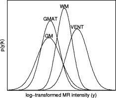
Distribution of voxel intensities in MR T2w image from Figure 1 modeled by fitted Gaussian probability density functions. Note large intensity variability and substantial intensity overlap between brain tissues, especially between developing gray matter (GM) and the germinal matrix (GMAT).

METHODS

EM Segmentation Framework

Expectation‐Maximization (EM) is a general technique for finding maximum likelihood estimates of model parameters in problems with missing data. In the context of brain MRI segmentation [Van Leemput et al., 1999b; Wells et al., 1996], the observed data are intensities y = {y(x ₁), y(x ₂), …, y(x _N)} of voxels x _i (i = 1, 2, …, N), the missing data are voxel labels c = {c(x ₁), c(x ₂), …, c(x _N)} (image segmentation), and the model parameters are K class‐conditional intensity distribution parameters θ = {θ₁, θ₂, …, θ_K}. The EM algorithm maximizes the likelihood of the observed data

(1)

by interleaving the expectation step (E‐step) which performs statistical classification of the observed data into K classes and the maximization step (M‐step) which updates the current parameter estimation.

Assuming that each voxel intensity y(x _i) is selected at random from one of K classes and each class k is modeled by a Gaussian distribution G with mean μ_k and variance σ_k [Wells et al., 1996], the probability density that class k generated voxel value y(x _i) is

(2)

and the class posterior probability p(k|x _i) computed in the E‐step is

(3)

where P(k) is a prior probability of tissue class k. The estimation of class distribution parameters θ_k = {μ_k, σ_k} is performed in the M‐step according to

(4)

and the intermediate segmentation of the image is given by voxel labels c(x _i) assigned using the maximum posterior probability rule.

(5)

Bias Correction

In MR imaging of the fetal brain, phased‐array coils are usually preferred over body coils as they can be placed much closer to the anatomy of interest [Levine et al., 2003; Prayer et al., 2004]. However, signal intensity in phased‐array MR images is not uniform and drops off quickly with the distance from the array. This is particularly an issue when the fetal head is positioned very close to the abdominal wall of the mother. Substantial intensity inhomogeneity, together with the bias field effect, can make the images difficult to interpret for a human reader and also cause tissue mislabeling in automated image segmentation.

Assuming a multiplicative bias model [Van Leemput et al., 1999a], intensity inhomogeneity b(x _i) is approximated by a linear combination of spatially smooth basis functions ϕ_j(x _i).

(6)

The coefficients a _j are recalculated in each iteration of the EM algorithm as the least‐squares fit to the difference between log‐transformed measured intensities y(x _i) and predicted intensities

(7)

calculated from intermediate estimates of class distribution parameters [Van Leemput et al., 1999a]. The bias‐corrected intensities y _c(x _i) = y(x _i) − b(x _i) replace the log‐transformed measured intensities y(x _i) in Eqs. (3) and (4) during the next iteration of the EM algorithm.

Probabilistic Atlas

The independent segmentation model from Eqs. (3) and (4) performs labeling of MRI voxels based solely on their intensities y(x _i) and assumes that different brain tissues are well separated in the intensity space. This, however, is not the case for clinical MR imaging of the fetal brain where the overlap of intensities between different tissue types is substantial, especially for developing cortical gray matter and the germinal matrix as shown in Figures 1 and 2. Moreover, the tissue labeling resulting from an intensity‐based segmentation of the fetal brain may not be anatomically feasible. To address these issues, a statistical atlas can be used as a source of spatial information to guide the local tissue labeling [Van Leemput et al., 1999b].

To create a statistical atlas of tissue distribution and a corresponding reference anatomy, an average shape and intensity image is first constructed from motion‐corrected MR volumes with normalized intensities. Using one subject as an initial reference (Fig. 3A), MR images are spatially normalized using a sequence of global linear registrations driven by maximization of normalized mutual information [Studholme et al., 1999] followed by multiple elastic deformations driven by maximization of mutual information [Viola and Wells, 1997] within a fixed reference region. An average shape model is obtained by averaging spatial transformations between the reference and each of the subject images (Fig. 3B). The subject images with normalized intensities are then transformed to the average shape space (Fig. 3C) and averaged to form a high quality average intensity image (Fig. 3D). These steps can be performed iteratively, each time using the average shape and intensity image as a new reference [Guimond et al., 2000].

Figure 3.

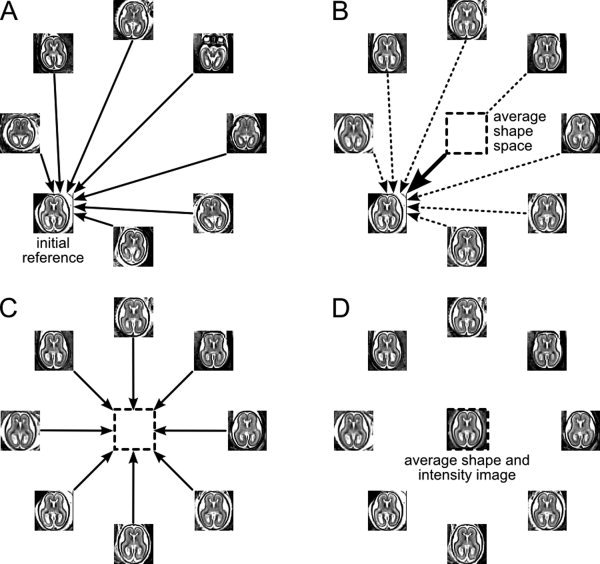
Building of the average shape and intensity model. Reconstructed and motion‐corrected subject images are warped to a reference image (A). The average shape model is obtained by averaging the spatial transformations between the subject images and the reference (B). The subject images with normalized intensities are transformed to the average shape space (C) and averaged to form an average intensity image (D). This image becomes a reference for the next iteration of the procedure (A).

After convergence of this procedure, tissue label maps obtained from manual segmentation of the subject images are transformed to the average shape space and normalized to form a probabilistic atlas. The atlas serves as a source of spatially varying tissue prior P _a(k|x _i) and replaces the location invariant P(k) during calculation of class posterior probabilities p(k|x _i) in Eq. (4) [Van Leemput et al., 1999b]. The average shape and intensity image is used as a high quality template for registration of new subject images to the space of the probabilistic atlas.

Neighborhood Constraints

A tissue label map resulting from the above segmentation scheme may be noisy or not anatomically feasible. It may, for example, contain an isolated voxel of one tissue surrounded by voxels of another tissue type. To eliminate such infeasible voxel label configurations, the segmentation process can be further constrained by introduction of neighborhood dependencies where the probability that a voxel belongs to a particular tissue depends on the tissue type of its neighbors. Using a simplified hidden Markov Random Field model [Zhang, 1992; Bach Cuadra et al., 2005], the prior probability of tissue type k at location x _i can be expressed as

(8)

where N _i is the neighborhood of voxel x _i and U(k|N _i) is the energy function dependent on the number of voxels from neighborhood N _i assigned to class k. This configuration encourages the voxel to be classified like the majority of its neighbors and promotes connected clusters of voxels from the same class. The normalizing factor Z(x _i) is used to ensure legitimate probability values of priors P _n(k|x _i). This optional neighborhood‐based prior can be combined with the prior P _a(k|x _i) derived from the probabilistic atlas to form one spatially varying prior

(9)

for estimation of tissue class probabilities.

RESULTS

Fetal Subjects

The following experiments were performed using clinical MR scans of 14 fetal subjects at gestational ages ranging from 20.57 to 22.86 weeks (see Fig. 4). These subjects were selected for manual tissue tracing from a larger pool collected at our institution over a period of five years. The mothers were referred for fetal MRI due to questionable abnormalities on prenatal ultrasound or a prior abnormal pregnancy. All women had normal fetal MRI and all newborns have had normal postnatal neurodevelopment.

Figure 4.

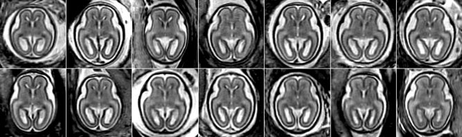
Axial views of rigidly aligned reconstructed MR T2w images of 14 fetal subjects (20.57–22.86 weeks GA) demonstrating variability in brain size and shape.

MR Image Acquisition and Processing

Clinical MR imaging was performed on a 1.5T scanner (GE Healthcare, Milwaukee, WI) using an eight‐channel torso phased‐array coil. For each subject, the position of the fetal head was first determined based on a low‐resolution three‐plane localizer sequence. Then, multiple stacks of single‐shot fast spin‐echo (SSFSE) T2w slice images (in plane resolution 0.469 mm × 0.469 mm, thickness ≈3 mm, no gap) were obtained in the approximately axial, sagittal and coronal planes with respect to the fetal brain. All slice images were acquired in an interleaved manner to reduce saturation of spins in adjacent slices. The MR sequence parameters (repetition time TR = 3000‐9000ms, echo time TE = 91 ms) were originally designed for clinical scans and were not adjusted for tissue segmentation in this study. To account for spontaneous fetal movement during scanning, image stacks of each subject were registered using the slice intersection motion correction (SIMC) technique [Kim et al., in press] and reconstructed into 3D volumes with isotropic resolution 0.469 mm × 0.469 mm × 0.469 mm.

Atlas Construction

The motion‐corrected volumes were manually segmented into regions of developing cortical gray matter, white matter, the germinal matrix, and ventricles as shown in Figure 5. The resulting tissue label maps were verified and corrected by pediatric neuroradiologists with expertise in fetal brain imaging. The intensities of the MR volumes were normalized before an average shape and intensity image was created. The manual segmentations of each subject were then transferred to the average shape space using nearest‐neighbor interpolation. A probabilistic atlas was created by averaging of tissue label maps extracted from manual delineations and smoothing of the resulting probability maps with a Gaussian kernel (σ = 1.5 mm) (see Fig. 6).

Figure 5.

Axial and coronal views of a reconstructed MR T2w image of a young fetal brain (22.14 weeks GA) with manually traced regions of developing gray matter, white matter, the germinal matrix and ventricles. [Color figure can be viewed in the online issue, which is available at wileyonlinelibrary.com.]

Figure 6.

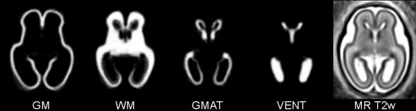
A probabilistic atlas for developing cortical gray matter (GM), white matter (WM), the germinal matrix (GMAT) and ventricles (VENT) constructed by spatial normalization of manual segmentations of MR T2w images of 14 fetal subjects at 20.57–22.86 weeks gestational age. The average shape and intensity image (MR T2w) is used as a high‐quality template for warping of new subject images to the space of the atlas.

Atlas‐Based EM Segmentation

For the purpose of automatic tissue segmentation, the reconstructed MR volume of each subject was warped to the average shape and intensity image associated with the probabilistic atlas. Then, the tissue probability maps were transferred from the atlas space to the original space of each subject using an inverse transformation. The number of classes for EM segmentation, K = 6, was selected to cover three types of developing brain tissues (GM, GMAT, WM), ventricles (VENT) and two types of nonbrain voxels (the surrounding fluid and the skull) with different intensity ranges. The distribution of intensity within each class k was modeled using a Gaussian distribution, θ_k = {μ_k, σ_k}. The class probabilities p(k|x _i) for brain tissues and ventricles were initialized with values P _a(k|x _i) from the probabilistic atlas and used to calculate the initial estimates of the intensity distribution parameters μ_k and σ_k according to Eq. (4). The initial values of μ_k and σ_k for the two non‐brain classes were copied from the estimates for GM and VENT, respectively. Because of the aforementioned intensity overlap between various developing tissues and the presence of other non‐brain structures (e.g., maternal organs) in the analyzed MR images, this atlas‐based initialization is the only feasible approach.

To evaluate the impact of the probabilistic atlas and the neighborhood constraints, automatic EM segmentation was performed in three modes:

• ‐ EM(P_n) where the probabilistic atlas was used only for initialization and further segmentation was constrained solely by the neighborhood prior,

• ‐ EM(P_a) where the prior tissue probabilities were taken from the probabilistic atlas,

• ‐ EM(P_a,P_n) where the combined prior from Eq. (9) was used to enforce neighborhood dependencies between voxel labels during atlas‐driven segmentation.

For each mode, the EM segmentation process was confined to regions of images where the atlas indicated a nonzero probability of any brain tissue. The bias field b(x) was modeled using polynomial functions ϕ_j(x) with degrees gradually increasing from zero to three. For each degree, EM iterations were performed until relative changes in the logarithm of the likelihood p(y|θ) were smaller than 10⁻⁴.

Segmentation Results

After convergence, the atlas‐based EM segmentation algorithm outputs an estimate of the bias field b(x), a bias‐corrected version y _c(x) of the original MR image y(x) fed to the algorithm and a tissue label map c(x) obtained by applying the maximum posterior probability rule [Eq. (5)] to class probability estimates p(k|x _i) from Eq. (3). Figure 7 presents typical results of automatic atlas‐based EM segmentation of a reconstructed MR T2w image of the young fetal brain (Fig. 7A) for all three segmentation modes. As the classification of voxels in the EM(P_n) mode is based only on intensity and intermediate labeling of the neighbors, it produces smooth but not necessarily feasible segmentations. In the example shown in Figure 7B, clusters of low intensity voxels inside the layer of the germinal matrix are incorrectly labeled as non‐brain structures. On the other hand, both atlas‐driven segmentation modes—EM(P_a) and EM(P_a,P_n)—yield more anatomically correct and overall similar results. The label map from EM(P_a,P_n) (Fig. 7D) is however more spatially coherent than the map produced by EM(P_a) (Fig. 7C).

Figure 7.

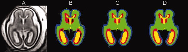
A reconstructed MR T2w image of a young fetal brain (21.57 weeks GA) (A) and results of its automatic segmentation in the EM(P_n) mode (B), the EM(P_a) mode (C), and the EM(P_a,P_n) mode (D). Label colors are: blue = gray matter, green = white matter, red = germinal matrix, yellow = ventricles. [Color figure can be viewed in the online issue, which is available at wileyonlinelibrary.com.]

Figure 8 further illustrates the effect of the neighborhood prior P_n on automatic atlas‐based EM segmentation of the fetal brain focusing on the area of the occipital lobe where thin layers of developing gray matter, white matter and the germinal matrix are adjacent. As this region is also a site of large anatomical variability even in young fetuses, registration of MR images in this area is challenging. This affects the local quality of the probabilistic atlas and leads to ambiguous priors P_a for multiple tissue types. These ambiguities can be addressed by the use of the neighborhood prior P_n in the EM(P_a,P_n) mode which enforces spatial consistency of tissue label maps by promoting connected structures. The neighborhood prior P_n also helps to eliminate mislabeled partial volume voxels at the interface between brain tissues with low T2w intensity (i.e., developing gray matter and the germinal matrix) and fluid with high T2w intensity. These voxels, indicated by arrows in Figures 8A and 8C, are incorrectly labeled as white matter in the EM(P_a) mode but almost completely eliminated in the EM(P_a,P_n) mode as shown in Figures 8B and 8D.

Figure 8.

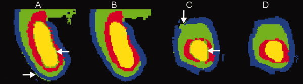
The effect of the neighborhood prior on automatic segmentation of fetal brain images in the area of the occipital lobe: (A and B) axial views of tissue label maps produces in the EM(P_a) and EM(P_a,P_n) modes, respectively, (C and D) coronal views of the same label maps. Label colors are: blue = gray matter, green = white matter, red = germinal matrix, yellow = ventricles. Arrows indicate examples of mislabeled partial volume voxels in the EM(P_a) mode. [Color figure can be viewed in the online issue, which is available at wileyonlinelibrary.com.]

Figure 9 demonstrates the results of automatic segmentation of a reconstructed MR T2w image with intensity inhomogeneity clearly visible in the coronal plane (Fig. 9A). This inhomogeneity arises from extreme proximity of one side of the fetal head to the maternal abdominal wall and the imaging coil. During segmentation, the intensity profile was estimated in the brain area and extrapolated to other parts of the image (Fig. 9B). The MR image with intensities corrected by the EM(P_a,P_n) segmentation algorithm is shown in Figure 9C and the final voxel labels are presented in Figure 9D.

Figure 9.

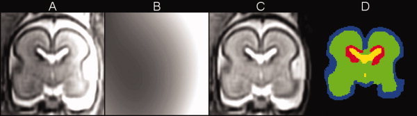
Automatic segmentation of a reconstructed MR T2w image with substantial intensity inhomogeneity: (A) original MR image y(x), (B) bias field estimation b(x), (C) bias‐corrected MR image y_c(x), and (D) labels c(x) from segmentation in the EM(P_a,P_n) mode. Label colors are: blue = gray matter, green = white matter, red = germinal matrix, yellow = ventricles. [Color figure can be viewed in the online issue, which is available at wileyonlinelibrary.com.]

Overall, visual inspection of the segmentation results for all study subjects indicates that the main tissue types in the fetal brain are delineated correctly and consistently, especially in the EM(P_a,P_n) mode. An example of 3D visualization of developing cortical gray matter, white matter, the germinal matrix and ventricles is shown in Figure 10.

Figure 10.

3D visualization of the main tissue types in the young fetal brain obtained from automatic segmentation of the average shape and intensity image. [Color figure can be viewed in the online issue, which is available at wileyonlinelibrary.com.]

Quantitative Validation

For quantitative validation, the results of automatic atlas‐based EM segmentation were evaluated in terms of the Dice similarity coefficient (DSC) [Dice, 1945] with respect to the reference manual segmentations. For any two regions A and B, the Dice similarity coefficient is defined as

(10)

and ranges from zero for complete dissimilarity to one for perfect overlap between A and B. Values of DSC above 0.7 are usually considered a satisfactory level of agreement between two segmentations [Zijdenbos et al., 1994; Xue et al., 2007].

Table I presents the summary of quantitative validation for the three modes of EM segmentation evaluated in this study. The DSC values were calculated for three developing tissue types in the fetal brain as well as ventricles and averaged over 14 subjects with gestational ages ranging from 20.57 to 22.86 weeks. The results from Table I demonstrate that the atlas‐based EM segmentation algorithm achieves good performance for all brain tissues, especially for developing gray matter, white matter and ventricles (DSC > 0.8). Overall, the best agreement between manual and automatic delineations, as measured by the DSC index, is achieved when both the anatomical prior P_a derived from the probabilistic atlas and the neighborhood prior P_n are used in the EM(P_a,P_n) mode. This allows for correct treatment of partial volume voxels at the interface between developing cortical gray matter and surrounding fluid as well as at the interface between the germinal matrix and ventricles.

Table I.

Values of Dice similarity coefficient (DSC) between manual and automatic segmentations for developing gray matter (GM), white matter (WM), the germinal matrix (GMAT) and ventricles (VENT) averaged over 14 fetal subjects (20.57–22.86 weeks GA)

Brain tissue or structure	Segmentation mode
	EM(Pn)	EM(Pa)	EM(Pa,Pn)
GM	0.79 ± 0.02	0.82 ± 0.02	0.82 ± 0.02
WM	0.85 ± 0.01	0.89 ± 0.02	0.90 ± 0.02
GMAT	0.65 ± 0.05	0.76 ± 0.05	0.77 ± 0.05
VENT	0.84 ± 0.04	0.89 ± 0.02	0.90 ± 0.02

DISCUSSION

In this article, we described methodology for automatic atlas‐based segmentation of individual tissues in the developing human fetal brain. The approach builds upon our earlier work on reconstruction of 3D images from in utero MR scans [Kim et al., in press; Rousseau et al., 2005, 2006] and a pilot study on atlas‐based segmentation of the germinal matrix from motion‐corrected clinical MRI [Habas et al., 2008]. As fetal MR imaging has become an important tool in evaluation of pregnancy, the presented methodology makes further use of standard clinical protocols allowing quantitative analysis of the developing brain using existing MR data.

To generate anatomically correct automatic segmentations, we created an in utero 3D statistical atlas of tissue distribution in the fetal brain incorporating multiple tissue classes such as developing gray and white matter as well as transient tissue types such as the germinal matrix. To relate manual delineations of multiple subjects and build the probabilistic atlas, we created an unbiased linear average shape and intensity model from the available set of training subjects. Although registration of reconstructed MR images was overall accurate, we are currently working on an approach where existing manual segmentations of subject volumes rather than MR images are collectively registered to create a reference anatomy [Habas et al., 2009a]. This may help us resolve some registration ambiguities between different tissues that appear with very similar intensities in relatively low‐contrast clinical MR scans. As a result, the quality of the probabilistic atlas is expected to improve, especially in challenging areas of the parietal and occipital lobes.

We applied the probabilistic atlas as a source of spatially varying prior for automatic EM segmentation of reconstructed and motion‐corrected MR images of the fetal brain. This well‐established algorithm is commonly used for brain segmentation in adults and has been previously applied for young children (e.g., [Murgasova et al., 2007]) and neonates (e.g., [Xue et al., 2007]). Here, we demonstrated that the EM‐based methodology can be further extended for automatic 3D delineation of developing tissues in the fetal brain, given an appropriate statistical atlas of the underlying anatomy. The EM segmentation algorithm also provides a convenient mechanism for model‐based estimation of intensity inhomogeneity which is a common issue in fetal MR imaging.

The quantitative validation in previous studies on segmentation of the developing brain anatomy has been limited. Overlap measures between manual and automatic segmentations were calculated using a single 2D slice [Prastawa et al., 2005] or three orthogonal slices [Xue et al., 2007] per subject. In this study, validation was performed using the entire brain volume for all study subjects and provided a more meaningful estimation of the segmentation performance. The average DSC values for developing gray and white matter as well as ventricles were very similar to those previously reported in other studies on segmentation of developing brains [Murgasova et al., 2007; Prastawa et al., 2005; Xue et al., 2007]. The somewhat lower but still satisfactory average DSC value and slightly higher DSC variance for the germinal matrix can be attributed to the fact that this transient tissue type undergoes rapid and individualized development for each fetal subject. Moreover, the boundary between the germinal matrix and white matter has very low contrast and its accurate and consistent identification is challenging even for experience neuroradiologists. Nonetheless, the overall good performance of the atlas‐based EM segmentation algorithm indicates that reliable morphometric measures of brain development can be automatically derived from clinical MR imaging.

Automatic segmentation of developing tissues from reconstructed 3D volumes makes use of 2D data collected through clinical MR scanning of fetal subjects. Reliable tissue delineation extends our knowledge of the normal brain development process and allows for further 3D volumetric and morphometric analysis of the fetal brain such as cortical thickness mapping [Chandramohan et al., 2009]. Moreover, efficient and reproducible processing of multiple volumes opens up the possibility for population‐based studies including investigation of early folding patterns [Habas et al., 2009b] and potentially others.

REFERENCES

- Bach Cuadra M, Cammoun L, Butz T, Cuisenaire O, Thiran J‐P ( 2005): Comparison and validation of tissue modelization and statistical classification methods in T1‐weighted MR brain images. IEEE Trans Med Imaging 24: 1548–1565. [DOI] [PubMed] [Google Scholar]
- Battin MR, Maalouf EF, Counsell SJ, Herlihy AH, Rutherford MA, Azzopardi D, Edwards AD ( 1998): Magnetic resonance imaging of the brain in very preterm infants: Visualization of the germinal matrix, early myelination, and cortical folding. Pediatrics 101: 957–962. [DOI] [PubMed] [Google Scholar]
- Brugger PC, Stuhr F, Lindner C, Prayer D ( 2006): Methods of fetal MR: Beyond T2‐weighted imaging. Eur J Radiol 57: 172–181. [DOI] [PubMed] [Google Scholar]
- Chandramohan D, Habas PA, Kim K, Glenn OA, Barkovich AJ, Studholme C ( 2009): Cortical thickness mapping of the human fetal brain in utero from motion‐corrected clinical MRI: Preliminary results. 15th Annual Meeting of the Organization for Human Brain Mapping, doi: 10.1016/S1053‐8119(09)70081‐3.
- Claude I, Daire J‐L, Sebag G ( 2004): Fetal brain MRI: Segmentation and biometric analysis of the posterior fossa. IEEE Trans Biomed Eng 51: 617–626. [DOI] [PubMed] [Google Scholar]
- Coakley FV, Glenn OA, Qayyum A, Barkovich AJ, Goldstein R, Filly RA ( 2004): Fetal MRI: A developing technique for the developing patient. Am J Roentgenol 182: 243–252. [DOI] [PubMed] [Google Scholar]
- Dice LR ( 1945): Measures of the amount of ecologic association between species. Ecology 26: 97–302. [Google Scholar]
- Girard N, Raybaud C, Poncet M ( 1995): In vivo MR study of brain maturation in normal fetuses. Am J Neuroradiol 16: 407–413. [PMC free article] [PubMed] [Google Scholar]
- Glenn OA, Barkovich AJ ( 2006): Magnetic resonance imaging of the fetal brain and spine: An increasingly important tool in prenatal diagnosis. Am J Neuroradiol 27: 1604–1611. [PMC free article] [PubMed] [Google Scholar]
- Grossman R, Hoffman C, Mardor Y, Biegon A ( 2006): Quantitative MRI measurements of human fetal brain development in utero. Neuroimage 33: 463–470. [DOI] [PubMed] [Google Scholar]
- Guimond A, Meunier J, Thirion J‐P ( 2000): Average brain models: A convergence study. Comput Vis Image Underst 77: 192–210. [Google Scholar]
- Habas PA, Kim K, Rousseau F, Glenn OA, Barkovich AJ, Studholme C ( 2008): Atlas‐based segmentation of the germinal matrix from in utero clinical MRI of the fetal brain. Med Image Comp Comput‐Assisted Interv LNCS 5241: 351–358. [DOI] [PMC free article] [PubMed] [Google Scholar]
- Habas PA, Kim K, Rousseau F, Glenn OA, Barkovich AJ, Studholme C ( 2009a): A spatio‐temporal atlas of the human fetal brain with application to tissue segmentation. Med Image Comp Comput‐Assisted Interv LNCS 5761: 289–296. [DOI] [PMC free article] [PubMed] [Google Scholar]
- Habas PA, Kim K, Rodriguez‐Carranza CE, Glenn OA, Barkovich AJ, Studholme C ( 2009b): Abnormal sulcal formation in fetuses with ventriculomegaly identified by surface curvature mapping from motion‐corrected clinical MRI. 15th Annual Meeting of the Organization for Human Brain Mapping, doi: 10.1016/S1053‐8119(09)70072‐2.
- Huppi PS, Warfield SK, Kikinis R, Barnes PD, Zientara GP, Jolesz FA, Tsuji MK, Volpe JJ ( 1998): Quantitative magnetic resonance imaging of brain development in premature and mature newborns. Ann Neurol 43: 224–235. [DOI] [PubMed] [Google Scholar]
- Inder TE, Warfield SK, Wang H, Huppi PS, Volpe JJ ( 2005): Abnormal cerebral structure is present at term in premature infants. Pediatrics 115: 286–294. [DOI] [PubMed] [Google Scholar]
- Jiang S, Xue H, Glover A, Rutherford M, Rueckert D, Hajnal JV ( 2007): MRI of moving subjects using multislice snapshot images with volume reconstruction (SVR): Application to fetal, neonatal, and adult brain studies. IEEE Trans Med Imaging 26: 967–980. [DOI] [PubMed] [Google Scholar]
- Kim K, Habas PA, Rousseau F, Glenn OA, Barkovich AJ, Studholme C (in press): Intersection‐based motion correction of multi‐slice MRI for 3D in utero fetal brain image formation. IEEE Trans Med Imaging, doi: 10.1109/TMI.2009.2030679. [DOI] [PMC free article] [PubMed] [Google Scholar]
- Kinoshita Y, Okudera T, Tsuru E, Yokota A ( 2001): Volumetric analysis of the germinal matrix and lateral ventricles performed using MR images of postmortem fetuses. Am J Neuroradiol 22: 382–388. [PMC free article] [PubMed] [Google Scholar]
- Kostovic I, Judas M, Rados M, Hrabac P ( 2002): Laminar organization of the human fetal cerebrum revealed by histochemical markers and magnetic resonance imaging. Cereb Cortex 12: 536–544. [DOI] [PubMed] [Google Scholar]
- Levine D, Stroustrup Smith A, McKenzie C ( 2003): Tips and tricks of fetal MR imaging. Radiol Clin N Am 41: 729–745. [DOI] [PubMed] [Google Scholar]
- Matsuzawa J, Matsui M, Konishi T, Noguchi K, Gur RC, Bilker, W , Miyawaki T ( 2001): Age‐related volumetric changes of brain gray and white matter in healthy infants and children. Cereb Cortex 11: 335–342. [DOI] [PubMed] [Google Scholar]
- Murgasova M, Dyet L, Edwards D, Rutherford M, Hajnal J, Rueckert D ( 2007): Segmentation of brain MRI in young children. Acad Radiol 14: 1350–1366. [DOI] [PubMed] [Google Scholar]
- Perkins L, Hughes E, Srinivasan L, Allsop J, Glover A, Kumar S, Fisk N, Rutherford M ( 2008): Exploring cortical subplate evolution using magnetic resonance imaging of the fetal brain. Dev Neurosci 30: 211–220. [DOI] [PubMed] [Google Scholar]
- Prastawa M, Gilmore JH, Lin W, Gerig G ( 2005): Automatic segmentation of MR images of the developing newborn brain. Med Image Anal 9: 457–466. [DOI] [PubMed] [Google Scholar]
- Prayer D, Brugger PC, Prayer L ( 2004): Fetal MRI: Techniques and protocols. Pediatr Radiol 34: 685–693. [DOI] [PubMed] [Google Scholar]
- Prayer D, Kasprian G, Krampl E, Ulm B, Witzani L, Prayer L, Brugger PC ( 2006): MRI of normal fetal brain development. Eur J Radiol 57: 199–216. [DOI] [PubMed] [Google Scholar]
- Rousseau F, Glenn OA, Iordanova B, Rodriguez‐Carranza CE, Vigneron D, Barkovich AJ, Studholme C ( 2008): A novel approach to high resolution fetal brain MR imaging. Med Image Comp Comput‐Assisted Interv LNCS 3749: 548–555. [DOI] [PubMed] [Google Scholar]
- Rousseau F, Glenn OA, Iordanova B, Rodriguez‐Carranza CE, Vigneron DB, Barkovich AJ, Studholme C ( 2006): Registration‐based approach for reconstruction of high‐resolution in utero fetal MR brain images. Acad Radiol 13: 1072–1081. [DOI] [PubMed] [Google Scholar]
- Rutherford M, Jiang S, Allsop J, Perkins L, Srinivasan L, Hayat T, Kumar S, Hajnal J ( 2008): MR imaging methods for assessing fetal brain development. Dev Neurobiol 68: 700–711. [DOI] [PubMed] [Google Scholar]
- Studholme C, Hill DLG, Hawkes DJ ( 1999): An overlap invariant entropy measure of 3D medical image alignment. Pattern Recognit 32: 71–86. [Google Scholar]
- Twickler DM, Magee KP, Caire J, Zaretsky M, Fleckenstein JL, Ramus RM ( 2003): Second‐opinion magnetic resonance imaging for suspected fetal central nervous system abnormalities. Am J Obstet Gynecol 188: 492–496. [DOI] [PubMed] [Google Scholar]
- Van Leemput K, Maes F, Vandermeulen D, Suetens P ( 1999a): Automated model‐based bias field correction of MR images of the brain. IEEE Trans Med Imaging 18: 885–896. [DOI] [PubMed] [Google Scholar]
- Van Leemput K, Maes F, Vandermeulen D, Suetens P ( 1999b): Automated model‐based tissue classification of MR images of the brain. IEEE Trans Med Imaging 18: 897–908. [DOI] [PubMed] [Google Scholar]
- Viola P, Wells WM ( 1997): Alignment by maximization of mutual information. Int J Comput Vis 24: 137–154. [Google Scholar]
- Wells WM, Grimson WEL, Kikinis R, Jolesz FA ( 1996): Adaptive segmentation of MRI data. IEEE Trans Med Imaging 15: 429–442. [DOI] [PubMed] [Google Scholar]
- Xue H, Srinivasan L, Jiang S, Rutherford M, Edwards AD, Rueckert D, Hajnal JV ( 2007): Automatic segmentation and reconstruction of the cortex from neonatal MRI. Neuroimage 38: 461–477. [DOI] [PubMed] [Google Scholar]
- Zijdenbos AP, Dawant BM, Margolin RA, Palmer AC ( 1994): Morphometric analysis of white matter lesions in MR images: Method and validation. IEEE Trans Med Imaging 13: 716–724. [DOI] [PubMed] [Google Scholar]
- Zhang J ( 1992): The mean field theory in EM procedures for Markov random fields. IEEE Trans Signal Process 40: 2570–2583. [DOI] [PubMed] [Google Scholar]