Dedicated breast CT: radiation dose for circle-plus-line trajectory

Abstract

Purpose: Dedicated breast CT prototypes used in clinical investigations utilize single circular source trajectory and cone-beam geometry with flat-panel detectors that do not satisfy data-sufficiency conditions and could lead to cone beam artifacts. Hence, this work investigated the glandular dose characteristics of a circle-plus-line trajectory that fulfills data-sufficiency conditions for image reconstruction in dedicated breast CT.

Methods: Monte Carlo-based computer simulations were performed using the GEANT4 toolkit and was validated with previously reported normalized glandular dose coefficients for one prototype breast CT system. Upon validation, Monte Carlo simulations were performed to determine the normalized glandular dose coefficients as a function of x-ray source position along the line scan. The source-to-axis of rotation distance and the source-to-detector distance were maintained constant at 65 and 100 cm, respectively, in all simulations. The ratio of the normalized glandular dose coefficient at each source position along the line scan to that for the circular scan, defined as relative normalized glandular dose coefficient $\left(R{D}_{g}N\right)$, was studied by varying the diameter of the breast at the chest wall, chest-wall to nipple distance, skin thickness, x-ray beam energy, and glandular fraction of the breast.

Results: The $R{D}_{g}N$ metric when stated as a function of source position along the line scan, relative to the maximum length of line scan needed for data sufficiency, was found to be minimally dependent on breast diameter, chest-wall to nipple distance, skin thickness, glandular fraction, and x-ray photon energy. This observation facilitates easy estimation of the average glandular dose of the line scan. Polynomial fit equations for computing the $R{D}_{g}N$ and hence the average glandular dose are provided.

Conclusions: For a breast CT system that acquires 300–500 projections over $2\pi$ for the circular scan, the addition of a line trajectory with equal source spacing and constant x-ray beam quality (kVp and HVL) and mAs matched to the circular scan, will result in less than 0.18% increase in average glandular dose to the breast per projection along the line scan.

INTRODUCTION

The clinical role of dedicated breast CT is being actively investigated.^{1, 2, 3} Prototype systems used in these clinical studies utilize a single circular source trajectory and cone-beam imaging with flat-panel detectors.^{4, 5} Multimodality SPECT/CT and PET/CT systems dedicated for breast imaging, wherein the CT component utilize a similar trajectory and cone-beam imaging have also been developed.^{6, 7} However, cone-beam imaging with a circular source trajectory does not satisfy the necessary conditions for data sufficiency.^{8, 9} Cone-beam imaging with such a trajectory could result in artifacts that manifest as variation in intensity and geometric distortion that are readily observed at locations away from the circular plane.^{10, 11} In our prior work,¹⁰ cone-beam artifacts at breast CT relevant imaging conditions were observed in noise-free and x-ray scatter-free simulations using a Hamming-windowed FDK-algorithm¹² with semiellipsoidal Defrise phantoms and surgical mastectomy based numerical phantoms. For the Defrise phantoms, quantitative inaccuracies increased with increase in linear attenuation coefficient difference between the tissues comprising the phantom and with increasing cone angle.¹⁰ This suggests that quantitative assessment in contrast-enhanced breast CT could be affected due to increase in linear attenuation coefficient resulting from contrast media uptake. Power spectral analysis of surgical mastectomy based numerical phantoms showed the presence of cone-beam artifacts.¹⁰ Specific to breast CT, Zeng et al.¹³ proposed a theoretically exact reconstruction based on two tilting arcs. Their simulations with a numerical breast phantom containing masses, calcifications, and fibers showed the potential to improve diagnostic performance with their method compared with a circular cone-beam CT scan using the FDK algorithm.¹³ Yang et al.¹¹ reported on mitigation of cone-beam artifacts with a circle plus partial helical trajectory and compared it with a circle plus line trajectory. Their numerical simulations showed that the shape of the objects were distorted near the nipple region with the circular cone-beam CT scan using FDK algorithm.¹¹ Although there are several source trajectories that can fulfill the necessary conditions for data sufficiency, we focused on the circle plus line trajectory as it can be implemented on existing prototype systems with relative ease by adding a translational stage for the x-ray source to obtain the line scan and with adaptive collimation. A key consideration¹¹ in such a scheme is the distribution of projection views between the circular and line scans for a given average glandular dose constraint and this requires knowledge of radiation dose for the line scan. Hence, this study was undertaken to determine the radiation dose properties through the normalized glandular dose conversion factor $\left(D_{g}N\right)$ for the line scan in dedicated breast CT. Other researchers have reported the average glandular dose to the breast in circular scan cone-beam dedicated breast CT.^{14, 15, 16}

METHODS AND MATERIALS

Monte Carlo simulations of radiation transport were performed by implementing a C++ program using the GEANT4 toolkit (version 9.3).¹⁷ The Livermore low energy physics model was used in this study and physical processes for x-ray photon interactions included Compton scattering, Rayleigh scattering, and photoelectric effect. For electrons, multiple scattering, ionization, and bremsstrahlung effects were included.

Simulation geometry

The simulation geometry for the circular scan is shown in Fig. 1. The semiellipsoidal breast is centered at the axis of rotation. The origin of the coordinate system used in these simulations is the intersection of the axis of rotation and the posterior (chest-wall) coronal plane of the breast. The distance between the source and axis of rotation (SAD) is 65 cm that corresponds to the geometry used in one clinical prototype system,⁴ and the source to detector distance (SDD) is 100 cm. For this imaging geometry, the chosen detector size (40 × 30 cm) corresponds to that used in clinical prototypes^{4, 5} and is sufficient to fully cover the largest breast diameter (18 cm) and chest-wall to nipple length (14 cm) considered in this work. The detector plane, i.e., the plane that contains the detector is parallel to the axis of rotation and orthogonal to the plane that contains the x-ray source and the axis of rotation. In our notation, the axis of rotation is the y-axis. A point on the detector is specified by two Cartesian coordinates: u and v, where the coordinate v is in the direction of y. The origin $(u,v)=(0,0)$ is such that, for each source position on the circular scan, the line that is orthogonal to the y-axis through the source position intersects the detector at $(u,v)=(0,0)$.

Figure 1.

Circular scan geometry used in Monte Carlo simulations (not drawn to scale). The breast is centered at the axis of rotation. If $(S_x,S_y,S_z)$ represents the source coordinates, then for all projections along the circular scan, $S_y=0$ and $\sqrt{S_x^2+S_z^2}=65\mathrm{cm}\mathrm{.}$

The range of breast diameters considered (14–18 cm) represent ∼95% of breast diameters observed in a study by Boone et al.¹⁴ We considered 2 and 4 mm thick skin in our simulations. The 2 mm skin thickness was chosen to match the skin thickness used in the study by Thacker for dosimetry in breast CT.¹⁵ The 4 mm skin thickness was included to be consistent with mammography¹⁸ and to match the skin thickness used in the study by Boone et al.¹⁴ Simulation parameters including the dimensions of the semiellipsoidal pendant breast used in the study are summarized in Table Table I.. The trajectory of the x-ray source during the circular scan is along the posterior coronal plane of the breast. If the coordinates of the x-ray source is represented as $(S_x,S_y,S_z)$, then for every projection along the circular scan, $S_y=0$ and $\sqrt{S_x^2+S_z^2}=65\mathrm{cm}$. The half-fan angle and half-cone angle are represented as α and β, respectively (Fig. 1).

Table I.

Summary of conditions used in Monte Carlo simulations.

Parameter	Value(s)
Source to rotational axis distance (SAD)	65 cm
Source to detector distance (SDD)	100 cm
Detector dimensions	40 cm × 30 cm
Diameter of breast at chest wall $\left(d\right)$	10, 14, and 18 cm
Chest wall to nipple lengtha$\left(L\right)$	$L=0.5d,0.75d\mathrm{,}1.0d$
Skin thickness $\left(t_s\right)$	2 and 4 mm
Glandular weight fraction $\left(f_g\right)$	0.02, 0.15, 0.5, and 1.0
Energy $\left(E\right)$	6–100 keV, 2 keV steps

^aMonte Carlo simulations were performed with $L=0.75d$ for all combinations of $d\mathrm{,}{t}_s,f_g,\mathrm{and}E.$ In addition, $L=0.5d$ and $L=1.0d$ were used in simulations for validation and to study the dependence of L for a fixed $d.$

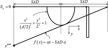
For the line scan, we considered two geometries, represented as A and B, which are shown in Fig. 2. For both geometries, at each source position along the line, the x-ray beam is defined by two half-cone angles, ${\beta }_1^{A/B}$ and ${\beta }_2^{A/B}$ in addition to the half-fan angle α. For both geometries, the ray that subtends the half-cone angle ${\beta }_2^{A/B}$ is the tangent to the elliptical surface of the breast in the $x-y$ plane. Also, for the source position corresponding to the circular plane, i.e., $S_y=0,$${\beta }_1^{A/B}=0,$ and ${\beta }_2^{A/B}=\beta ,$ where β is the half-cone angle of the circular scan. In geometry A, for each source position along the line scan, the ray that subtends the half-cone angle ${\beta }_1^A$ is incident on the top row of the detector. In geometry B, the ray that subtends the half-cone angle ${\beta }_1^B$ intersects the circular scan trajectory, at each source position along the line scan. The maximum length of the line scan, $y^{\text{max}}$ needed to achieve data-sufficiency can be calculated as per Eq. 1 from the slope of the line tangent to the ellipse that intercepts the circular trajectory (Fig. 3) and the derivation is included in Appendix A.

$$y^{\text{max}}=\frac{2\mathit{SAD}L}{\sqrt{\mathit{SA}{D}^2-{\left(\frac{d}{2}\right)}^2}}$$ (1)

In our Monte Carlo simulations, we translated the line source by n steps of $\Delta y$, such that $n\Delta y<y_{\text{max}}<(n+1)\Delta y$ so that a small amount of breast tissue excluding the skin was always irradiated to facilitate determination of glandular dose. In one circular scan clinical prototype system⁴ that features a (SAD) of 65 cm, 300 projections are acquired over $2\pi$ radians, resulting in a chord length between two successive projections of 1.361 cm. The optimal spacing between successive x-ray source positions along the line scan $\Delta y$ is subject of ongoing research; hence, we used $\Delta y=1.361\mathrm{cm}$ in our Monte Carlo simulations.

Figure 2.

Two geometries considered for the line scan (not drawn to scale). $S_y=0$ represents the source position during the circular scan and $S_y=y$ the source position during the line scan, when the source is translated by the distance y. In geometry A, the ray that subtends the half-cone angle ${\beta }_1^A$ is incident on the top row of the detector. In geometry B, the ray that subtends the half-cone angle ${\beta }_1^B$ intersects the circular scan trajectory.

Figure 3.

The maximum length of the line scan $y^{\text{max}}$ was computed from the slope of the tangent to the ellipse and was related to the source to axis of rotation distance, $\mathit{SAD}$, the diameter of the breast at the chest wall, d, and the chest wall to nipple distance, L.

In order to fulfill data-sufficiency conditions, for any given source position on the line scan, i.e., $S_y\ne 0$, we need to know the line integrals for all detector locations that are anterior (toward nipple) to the projection of the circle.^{19, 20} On the detector plane, the projection of the circle is a parabola. Mathematical treatment of the data-sufficiency conditions and their relevance to the geometries considered are included in Appendix B.

Monte Carlo simulations and analysis

Monte Carlo simulations were performed with monoenergetic x-ray photons using the method in Boone,²¹ with the correction factor that apportions the dose to glandular tissue $\left(G_{\mathit{dep}}\right)$ on a per interaction basis as described by Wilkinson and Heggie.²² The $G_{\mathit{dep}}$ factor was determined as per Boone and is shown in Eq. 2.

$$G_{\mathit{dep}}=\frac{f_g{\left({\mathrm{\mu }}_{\mathrm{en}}/\mathrm{\rho }\right)}_g}{f_g{\left({\mathrm{\mu }}_{\mathrm{en}}/\mathrm{\rho }\right)}_g+(1-f_g){\left({\mathrm{\mu }}_{\mathrm{en}}/\mathrm{\rho }\right)}_a}$$ (2)

In Eq. 2, $f_g$ represents the glandular weight fraction, ${({\mu }^{\mathit{en}}/\rho )}_g$ and ${({\mu }^{\mathit{en}}/\rho )}_a$ the energy-dependent mass attenuation coefficients of glandular and adipose tissue, respectively. Skin and homogenous breast tissue with the composition provided by Hammerstein et al.²³ were used. Although the distribution of adipose and fibroglandular tissue in the breast is heterogeneous, it has been shown that the use of a homogenous breast model with equivalent glandular fraction is sufficient for determining radiation dose.²⁴ At each source position along the line scan and for each geometry, a total of 1152 Monte Carlo simulations (3 breast diameters × 2 skin thicknesses × 4 glandular fractions × 48 x-ray photon energies), each comprising 1 × 10⁶ x-ray photons were tracked and the energy deposited E_dep corrected for G_dep was recorded. The dependence on chest wall to nipple length $\left(L\right)$ was studied for both geometries with $L=0.5d$ and $L=1.0d$ for a 14 cm diameter breast with 2 mm skin and $f_g=0.15$, resulting in additional 192 (2 geometries × 2 chest wall to nipple lengths × 48 x-ray photon energies) Monte Carlo simulations. In order to determine the statistical precision, Monte Carlo simulations for the smallest breast diameter $(d=10\mathrm{cm}\mathrm{,}{t}_s=2\mathrm{mm}\mathrm{,}{f}_g=0.5)$ at source position $S_y=0$ was repeated five times at 10, 30, and 100 keV, each with 10⁶ x-ray photons, and the product E_dep × G_dep were recorded. For each keV considered, the coefficient of variation (COV) was computed from the mean and standard deviation of the recorded E_dep × G_dep from five runs.

Data from Monte Carlo simulations were retrieved and the energy-dependent normalized glandular dose coefficients $D_{g}N\left(E\right)$ were computed^{15, 21} as in Eq. 3 using a matlab (Version 7.7.0 R2008, MathWorks Inc., Natick, MA) program for each source position, breast dimension, skin thickness, and glandular fraction.

$$D_{g}N\left(E\right)=\frac{\mathrm{Area}}{\mathrm{Mass}}{E}_{\mathit{dep}}{G}_{\mathit{dep}}\phi \left(E\right)1.6021\times {10}^{-8}$$ (3)

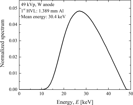
In Eq. 3, Area represents the cross-sectional area of the x-ray beam at axis of rotation in units of mm², Mass represents the glandular mass of the breast in grams, $\phi \left(E\right)$ represents the photons fluence per unit exposure in units of photons/(mm²R), and the constant $1.6021\times {10}^{-8}$ is in units of (mRad g)/keV as described by Boone.²¹ The computed $D_{g}N\left(E\right)$ were in units of mRad/R and were converted to S.I. units of mGy/mGy. Thus, the product of measured air kerma in units of mGy and without any phantom at SAD and $D_{g}N\left(E\right)$ provide the average glandular dose (AGD) to the breast in units of mGy. The cross-sectional area of the x-ray beam at the axis of rotation for each source position needed for computing $D_{g}N\left(E\right)$ was determined in a manner similar to that in Appendix A. The polyenergetic normalized glandular dose coefficient $D_g{N}^{\mathit{CT}}$ was determined by weighting the monoenergetic $D_{g}N\left(E\right)$ coefficients with the polyenergetic x-ray spectrum using the method described by Boone.²⁵ A 49 kVp tungsten anode spectrum (Fig. 4) with a 1st half-value layer of 1.389 mm of Al and mean energy of 30.4 keV was simulated using SRS-78 by IPEM²⁶ and was used to compute the $D_g{N}^{\mathit{CT}}$. This spectrum approximates that used by one clinical prototype system for which $D_g{N}^{\mathit{CT}}$ has been reported.¹⁶ The simulated spectrum was in 0.5 keV intervals and did not contain characteristic edges. Hence, the x-ray spectrum was resampled to 2 keV intervals to match our Monte Carlo simulations and was used to determine $D_g{N}^{\mathit{CT}}$. For validation of our Monte Carlo simulations with published data,¹⁶ the simulation geometry was modified to include the patient protective cup with the stated dimensions. However, the water phantom representing the torso was not included as its dimensions were not provided in that study.¹⁶ Monoenergetic $D_{g}N\left(E\right)$ coefficients were determined with chest wall to nipple length $L=0.5d,0\mathrm{.}75d\mathrm{,}1\mathrm{.}0d,$ breast diameter $d=10,14\mathrm{,}18\mathrm{cm}\mathrm{,}$ skin thickness $t_s=1.45\mathrm{mm}\mathrm{,}$ and glandular weight fraction $f_g=0.5\mathrm{,}1\mathrm{.}0$. $D_g{N}^{\mathit{CT}}$ values computed using a 49 kVp tungsten anode spectrum with a 1st half-value layer of 1.32 mm of Al to match the conditions in the published study.¹⁶

Figure 4.

A 49 kVp tungsten anode x-ray spectrum with 1st HVL of 1.389 mm of Al was used for $D_g{N}^{\mathit{CT}}$ computation. The spectrum is normalized to unit area.

The average glandular dose to the breast at each source position along the line scan was studied by the relative normalized glandular dose coefficient, $R{D}_{g}N\left(y\right)$, which we defined as the ratio of the normalized glandular dose coefficient at source position $S_y=y$ to that for $S_y=0$ .

$$R{D}_{g}N\left(y\right)=\frac{D_{g}N\left(y\right)}{D_{g}N\left(0\right)}$$ (4)

In Eq. 4 the dependence on energy E is implicit to simplify the exposition. The benefit of the chosen metric is readily apparent, as it provides the ratio of the $D_{g}N$ coefficient at each source position along the line scan to that for a circular scan. Thus by definition, $R{D}_{g}N\left(0\right)=1$. Additional analysis were performed using $R{D}_{g}N\left(k{y}^{\text{max}}\right)$, and is defined below

$$R{D}_{g}N\left(k{y}^{\text{max}}\right)=\frac{D_{g}N\left(k{y}^{\text{max}}\right)}{D_{g}N\left(0\right)}\mathrm{where}k\in [0,1)$$ (5)

RESULTS

Validation

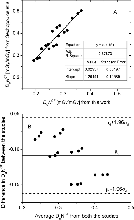
The coefficients of variation (COV) in E_dep × G_dep determined from five runs with the smallest breast diameter considered $(d=10\mathrm{cm}\mathrm{,}{t}_s=2\mathrm{mm}\mathrm{,}{f}_g=0.5)$ at 10, 30, and 100-keV were 0.25, 0.12, and 0.13%, respectively. The small $\mathit{COV}$ values indicate that the choice of 10⁶ x-ray photons provided sufficient statistical precision. The polyenergetic normalized glandular dose coefficients $D_g{N}^{\mathit{CT}}$ determined with a 49 kVp, tungsten anode x-ray spectrum (1st HVL: 1.32 mm of Al) that included the patient protective cup were compared with published data,¹⁶ and is shown in Fig. 5. In Fig. 5a, the linear fit (OriginPro 8.6, OriginLab Corp., Northampton, MA) of the data between the two studies is shown. Although the fit indicated reasonable correlation $(\mathit{adj}.r^2=0.88)$, the non zero intercept $(a=0.03\pm 0.03)$ and non unity slope $(b=1.29\pm 0.03)$ indicated that the data between the two studies were different and this was confirmed by statistical analysis $(p<{10}^{-9})$. In Fig. 5b, the Bland-Altman²⁷ plot is shown, where ${\mu }_d$ represents the mean difference between the studies and ${\sigma }_d$ the standard deviation of the difference between the studies. The differences between the two studies were within the 95% confidence intervals indicating good agreement between the studies. Our simulations used 2 keV energy bins as opposed to 0.5 keV energy bins.¹⁶ Our simulations also did not include the volume of water used to represent the body, which were included in the study by Sechopoulos.¹⁶ Considering these differences, the correlation and agreement between our results and published data¹⁶ are reasonable.

Figure 5.

Validation of our Monte Carlo simulation results with data published by Sechopoulos et al. (Ref. ¹⁶) A. Linear fit of $D_g{N}^{\mathit{CT}}$ from this work to published data shows reasonable correlation (adjusted $r^2=0.88$). B. Bland-Altman plot shows good agreement, where ${\mu }_d$ represents the mean difference between the studies and ${\sigma }_d$ the standard deviation of the difference between the studies.

Monoenergetic $D_{g}N\left(E\right)$

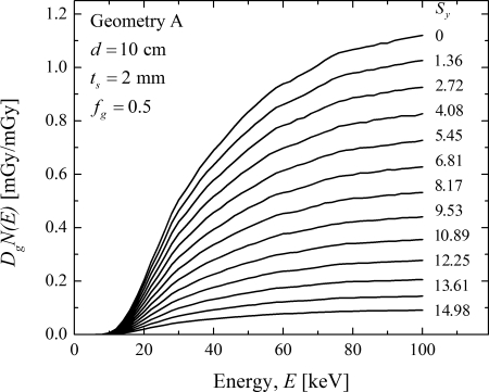
In Fig. 6, the monoenergetic $D_{g}N\left(E\right)$ coefficients are plotted as a function of energy at each source position along the line scan for geometry A. The plots are in the same order as the legend showing the source position $S_y$. At each keV, a monotonic decreasing trend in $D_{g}N\left(E\right)$ is observed when the x-ray source is translated away from the chest wall. This trend is consistent with the theoretical expectation as the volume of breast tissue irradiated decreases when the x-ray source is translated away from the chest wall. Similar trends were also observed with geometry B and when breast properties $(d,t_s,f_g)$ were varied and hence are not shown. The rest of the analysis was performed using the relative normalized glandular dose coefficient, either $R{D}_{g}N\left(y\right)$ or $R{D}_{g}N\left(k{y}^{\text{max}}\right)$, which were defined in Eqs. 4, 5, respectively.

Figure 6.

Monoenergetic $D_{g}N\left(E\right)$ plotted as a function of energy at each source position along the line scan for geometry A. The plots are in the same order as the legend showing the source position $S_y$. At each keV, there a monotonic decreasing trend in $D_{g}N\left(E\right)$ is observed when the x-ray source is translated away from the chest wall. Similar trend was also observed with geometry B and when breast properties $(d,t_s,f_g)$ were varied.

Monoenergetic $R{D}_{g}N\left(y\right)$

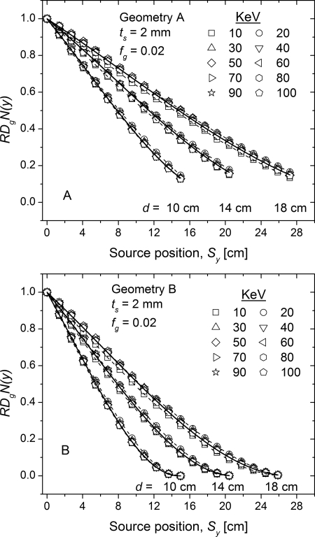
In Fig. 7, the monoenergetic $R{D}_{g}N\left(y\right)$ is plotted as a function of source position $S_y$ along the line scan for 10, 14, and 18 cm diameter breasts with 2 mm skin thickness and 2% glandular fraction. While the simulations were performed in 2 keV intervals, for clarity the plots are shown in 10 keV intervals. For each breast diameter and at each source position, the ten energy intervals were averaged and fitted with a third order polynomial. The fitted curves for each breast diameter are shown as solid lines and the fit parameters are summarized in Table Table II.. The dashed lines represent the maximum deviation from the fit, which occurred at 10 and 20 keV. At a given source position along the line scan $(S_y\ne 0)$, $R{D}_{g}N\left(y\right)$ increases with increasing breast diameter, as the volume of breast tissue irradiated increases with increasing breast diameter. Also, $R{D}_{g}N\left(y\right)$ with geometry B indicated faster roll-off with source position away from the chest wall $\left(S_y\right)$ than geometry A, implying that the radiation dose along the line scan is lower with geometry B than geometry A. This is consistent with theoretical expectation as at each source position along the line scan $(S_y\ne 0)$, the volume of breast irradiated will always be larger with geometry A than geometry B.

Figure 7.

Monoenergetic relative normalized glandular dose coefficient $R{D}_{g}N\left(y\right)$ plotted as a function of source position $S_y$ for 10, 14, and 18 cm diameter breasts with 2 mm skin thickness and 2% glandular fraction.

Table II.

Fit coefficients of the third-order polynomial $R{D}_{g}N\left(y\right)=1-ay-b{y}^2+c{y}^3$ used in Fig. 7 for both geometries.

	Fit parameters
Breast diameter	a	b	c	$\mathrm{adjusted}{r}^2$
Geometry A
10 cm	$0.06033$	$0.00104$	$7.97537\times {10}^{-5}$	1.0
14 cm	$0.03912$	$7.97262\times {10}^{-4}$	$3.46653\times {10}^{-5}$	1.0
18 cm	$0.03195$	$3.08884\times {10}^{-4}$	$1.23063\times {10}^{-5}$	0.99999
Geometry B
10 cm	$0.08661$	$0.00198$	$2.2055\times {10}^{-4}$	1.0
14 cm	$0.05952$	$0.00112$	$8.04996\times {10}^{-5}$	0.99999
18 cm	$0.04541$	$6.77777\times {10}^{-4}$	$3.6553\times {10}^{-5}$	0.99998

The influence of glandular fraction $f_g$ on $R{D}_{g}N\left(y\right)$ was studied and is shown in Fig. 8. The $R{D}_{g}N\left(y\right)$ values determined with 2% glandular breast across all breast diameters, all source positions, and across all energies (10 keV bins) are plotted against the corresponding $R{D}_{g}N\left(y\right)$ values determined with 15, 50, and 100% glandular fractions. The data were fit to linear equations with unit slope. The intercept and the adjusted $r^2$ values are shown in the legend. The near-zero values for the intercept and the near-unity values for the adjusted $r^2$ indicate that the $R{D}_{g}N\left(y\right)$ is independent of glandular fraction, $f_g$. Statistical analysis with paired t-test confirmed these observations $(p>0.9)$ for all cases. Similar linear fits to data with 4 mm skin thickness also indicated that the $R{D}_{g}N\left(y\right)$ was independent of glandular fraction, $f_g$ and hence are not shown for conciseness.

Figure 8.

Glandular fraction dependence of $R{D}_{g}N\left(y\right)$. The $R{D}_{g}N\left(y\right)$ determined with $f_g=0.02$ is plotted against that determined at other glandular fractions $(f_g=0.15,0\mathrm{.}5\mathrm{,}1\mathrm{.}0)$. The data were fit to a line with unity slope. The intercept $\left(c\right)$ and adjusted $r^2$ values are shown in the legend. For both geometries, the near-zero intercept implies that $R{D}_{g}N\left(y\right)$ is independent of glandular fraction.

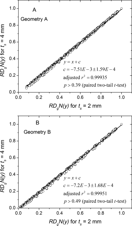
The influence of skin thickness $t_s$ on $R{D}_{g}N\left(y\right)$ was studied and is shown in Fig. 9. The $R{D}_{g}N\left(y\right)$ values determined with 2 mm skin across all breast diameters, source positions and glandular fractions are plotted against the corresponding $R{D}_{g}N\left(y\right)$ values determined with 4 mm skin. The data were fit to a linear equation with unit slope and the intercept and adjusted $r^2$ value are shown in the legend. The near-zero values for the intercept and the near-unity values for the adjusted $r^2$ indicate that the $R{D}_{g}N\left(y\right)$ is independent of skin thickness and was confirmed by paired t-test $(p>0.49)$.

Figure 9.

Skin thickness dependence of $R{D}_{g}N\left(y\right)$. The $R{D}_{g}N\left(y\right)$ determined with $t_s=2\mathrm{mm}$ is plotted against that determined at $t_s=4\mathrm{mm}$. The data were fit to a line with unity slope. The intercept $\left(c\right)$ and adjusted $r^2$ values are shown in the legend. For both geometries, the near-zero intercept implies that $R{D}_{g}N\left(y\right)$ is independent of skin thickness.

Polyenergetic $R{D}_g{N}^{\mathit{CT}}\left(y\right)$

In Figs. 789, the monoenergetic $R{D}_{g}N\left(y\right)$ were analyzed. Figures 89 show that the $R{D}_{g}N\left(y\right)$ was independent of skin thickness and glandular fraction, and hence the polyenergetic $R{D}_g{N}^{\mathit{CT}}\left(y\right)$ will also be independent of skin thickness and glandular fraction. However, Fig. 7 showed a small dependence on keV, particularly at low energies. In practice, the x-ray spectrum is polyenergetic and the x-ray beam quality (kVp and HVL) is usually maintained the same during acquisition of projections. Hence, the $R{D}_g{N}^{\mathit{CT}}\left(y\right)$ was determined using a 49 kVp x-ray spectrum (Fig. 4) and was analyzed in terms of source position $S_y$ along the line scan for both geometries (Fig. 10). For each breast diameter and at each source position, there are 8 data points $(4f_g\times 2t_s)$. The solid lines represent the third-order polynomial fit and the fit coefficients are summarized in Table Table III.. Similar to the trends observed with monoenergetic $R{D}_{g}N\left(y\right)$ shown in Fig. 7, the polyenergetic $R{D}_g{N}^{\mathit{CT}}\left(y\right)$ increases with increasing breast size at a given source position along the line scan $(S_y\ne 0)$, and geometry B indicated a faster roll-off with source position away from the chest wall $\left(S_y\right)$ than geometry A. These trends are consistent with theoretical expectations.

Figure 10.

Polyenergetic relative glandular dose coefficient $R{D}_g{N}^{\mathit{CT}}\left(y\right)$ determined for a 49 kVp (1^st HVL: 1.389 mm of Al) plotted as a function of source position $S_y$ along the line scan. For each breast diameter and at each source position, there are 8 data points $(4f_g\times 2t_s)$. Solid lines represent third-order polynomial fit.

Table III.

Coefficients of the third-order polynomial fit of the polyenergetic $R{D}_g{N}^{\mathit{CT}}\left(y\right)$ of the form $R{D}_g{N}^{\mathit{CT}}\left(y\right)=1-ay-b{y}^2+c{y}^3$ determined with a 49 kVp x-ray spectrum (1st HVL: 1.389 mm of Al). The fit corresponds to Fig. 10.

	Fit parameters
Breast diameter (cm)	a	b	c	$\mathrm{adjusted}{r}^2$
Geometry A
10	$0.05839$	$0.00124$	$8.46246\times {10}^{-5}$	0.99996
14	$0.03991$	$6.78237\times {10}^{-4}$	$3.06939\times {10}^{-5}$	0.9999
18	$0.03068$	$3.72287\times {10}^{-4}$	$1.31811\times {10}^{-5}$	0.99995
Geometry B
10	$0.08357$	$0.00246$	$2.39446\times {10}^{-4}$	0.99989
14	$0.05722$	$0.00133$	$8.50915\times {10}^{-5}$	0.99994
18	$0.04391$	$7.54892\times {10}^{-4}$	$3.72787\times {10}^{-5}$	0.99994

$R{D}_{g}N\left(k{y}^{\text{max}}\right)$

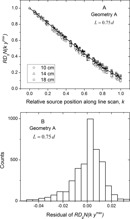
Figure 11 shows the monoenergetic relative glandular dose coefficient analyzed as per Eq. 5 for geometry A. In Fig. 11a, $R{D}_{g}N$ is plotted as a function of relative source position along line scan $(k=S_y/y^{\text{max}})$. For each breast diameter and at each source position there are 80 data points $(4f_g\times 2t_s\times 10\mathrm{energies})$. The solid line is a third-order polynomial fit obtained by combining the data across all diameters, skin thicknesses, glandular fractions, and 10 x-ray photon energies. The fit coefficients are summarized in Table Table IV.. This analysis shows $R{D}_{g}N\left(k{y}^{\text{max}}\right)$ did not show a marked dependence on breast diameter, skin thickness, glandular fraction, and x-ray photon energy. In Fig. 11b, the histogram of the residual from the polynomial fit is shown. The mean (2.12 × 10⁻⁴) and median (1.6 × 10⁻³) residual were less than 0.005 implying that the average glandular dose along the line scan can be estimated on average with 0.5% accuracy relative to that of the circular scan.

Figure 11.

(a) Monoenergetic relative glandular dose coefficient $R{D}_{g}N$ plotted as a function of relative source position along line scan $(k=S_y/y^{\text{max}})$ corresponding to Eq. 3 for geometry A. For each breast diameter and at each source position, there are 80 data points $(4f_g\times 2t_s\times 10\mathrm{energies})$. The solid line is a third-order polynomial fit obtained by combining the data across all diameters, skin thicknesses, glandular fractions, and 10 x-ray photon energies. (b) Histogram of the residual from the polynomial fit.

Table IV.

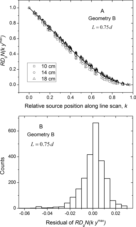
Coefficients of the third-order polynomial fit of $R{D}_{g}N\left(k{y}^{\text{max}}\right)$ of the form $R{D}_{g}N\left(k{y}^{\text{max}}\right)=1-ak-b{k}^2+c{k}^3$. The fit coefficients correspond to data in Figs. 11a, 12a.

	Fit parameters
Geometry	a	b	c	$\mathrm{Adjusted}{r}^2$
A	0.87987	0.26215	0.27797	0.99957
B	1.25477	0.51556	0.77068	0.99961

Figure 12 show the corresponding plots for geometry B, where Fig. 12a shows the $R{D}_{g}N\left(k{y}^{\text{max}}\right)$ plotted as a function of relative source position k along the line scan and Fig. 12b the histogram of the residual from the polynomial fit. The polynomial fit coefficients are summarized in Table Table IV.. From the histogram of the residual, it is apparent that the average glandular dose along the line scan can be estimated with similar accuracy as geometry A. Similar analysis with the polyenergetic $R{D}_g{N}^{\mathit{CT}}\left(k{y}^{\text{max}}\right)$ for both geometries did not show a marked dependence on breast diameter, skin thickness and glandular fraction, and hence are not shown for conciseness.

Figure 12.

(a) Monoenergetic relative glandular dose coefficient $R{D}_{g}N$ plotted as a function of relative source position along line scan for geometry B. The solid line is a third-order polynomial fit obtained by combining the data across all diameters, skin thicknesses, glandular fractions, and 10 x-ray photon energies. (b) Histogram of the residual from the polynomial fit.

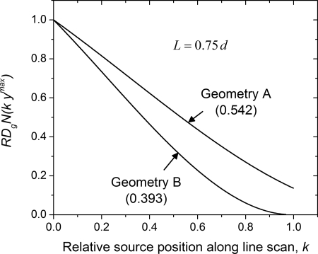
Figure 13 shows the comparison between the geometries in terms of $R{D}_{g}N\left(k{y}^{\text{max}}\right)$. The lines are the polynomial fits with coefficients summarized in Table Table IV.. The area under each curve was determined by integration along the relative source position k, and are reported within parenthesis for the corresponding geometry. The computed area indicates geometry B results in approximately 15% reduction in average glandular dose along the line scan than geometry A, when air kerma per projection and sampling along the line scan are maintained the same for both geometries.

Figure 13.

Comparison of $R{D}_{g}N\left(k{y}^{\text{max}}\right)$ shows geometry B results in lower radiation dose than geometry A when air kerma per projection and sampling along the line scan are maintained the same for both geometries. The value within parenthesis indicates the area under the curve for the corresponding geometry.

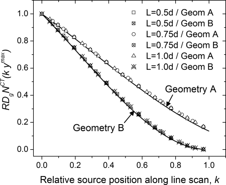
In Fig. 14, the symbols represent the polyenergetic $R{D}_g{N}^{\mathit{CT}}\left(k{y}^{\text{max}}\right)$ computed for the 49 kVp x-ray spectrum with breast parameters of $d=14$, $f_g=0.15$, and $t_s=2$ mm. For this fixed breast diameter d, the chest-wall to nipple length L was varied to study its dependence on $R{D}_g{N}^{\mathit{CT}}\left(k{y}^{\text{max}}\right)$. The solid lines are the polynomial fits generated from monoenergetic $R{D}_{g}N\left(k{y}^{\text{max}}\right)$ with their coefficients summarized in Table Table IV.. The observed agreement suggest that the fit coefficients are also valid for polyenergetic $R{D}_g{N}^{\mathit{CT}}\left(k{y}^{\text{max}}\right)$ and when the chest-wall to nipple length is varied.

Figure 14.

The plots show that the fit equations are also valid for polyenergetic $R{D}_g{N}^{\mathit{CT}}\left(k{y}^{\text{max}}\right)$ when the chest-wall to nipple length is varied for a fixed breast diameter. The symbols represent data points computed for breasts with $d=14$, $f_g=0.15$, and $t_s=2$ mm.

DISCUSSION

This study considered two imaging geometries for the line scan and these geometries along with the circular scan fulfill the necessary conditions for data-sufficiency. While the results demonstrate that geometry B could reduce radiation dose compared to geometry A, there are additional considerations such as extrapolation requirements during reconstruction that could affect image quality. Based purely on data-sufficiency conditions as described in Appendix B, it can be observed that the geometry A provides all of (and more than) the required data, while geometry B may require extrapolation. In the worst case scenario that occurs at $S_y=y_{\text{max}}$, $d=18\mathrm{cm}$ and $L=1.0d$, projection data may need to be interpolated over 5.5 mm at the periphery of the cylindrical field of view near the nipple. It is important to note that for a semiellipsoidal breast, this region will most likely occur outside the breast and hence would be irrelevant. The choice of imaging geometry and optimal sampling along the line scan are subjects of ongoing research.

Our Monte Carlo simulations used monoenergetic x-ray photons from a point source, and hence do not include the effect of focal spot size, shape, and x-ray photon distribution that could influence the x-ray beam profile. This choice is consistent with previous studies on radiation dose estimation in dedicated breast CT.^{14, 15, 16} Polyenergetic $D_g{N}^{\mathit{CT}}$ values were determined using the x-ray spectrum²⁶ simulated with a target (anode) angle of ${16}^{\circ }$ that corresponds to that of the x-ray tube used in one clinical prototype.⁴ No additional changes to the x-ray beam profile were made.

Our study considered 2 and 4-mm skin thickness, and glandular weight fractions of 0.02, 0.15, 0.5, and 1.0. Analyzing dedicated breast CT clinical images, recent reports on skin thickness²⁸ and glandular fraction²⁹ indicate that the mean skin thickness to be 1.45 mm and the mean glandular volume fraction excluding the skin to be 0.143. From Figs. 89, it is observed that the chosen metric of relative normalized glandular dose coefficient, $R{D}_{g}N\left(y\right)$ was independent of skin thickness and glandular fraction. This suggests that the provided data may also be suitable for the reported skin thickness and glandular fraction. Our study did not include the patient protective cup that is used in one clinical prototype¹⁶ except for the validation study. This choice was made so as to minimize the differential attenuation and hence variability in beam hardening that would arise when the x-ray source is translated during the line scan. Further, to our knowledge, the clinical prototype system developed by Boone et al.^{5, 14} does not include such a protective cup.

Since other researchers have reported on normalized glandular dose coefficients for cone-beam dedicated breast CT employing a single circular scan,^{14, 15, 16} we chose the metric of relative normalized glandular dose coefficient along the line scan for analysis. Further, by stating this metric $R{D}_{g}N\left(k{y}^{\text{max}}\right)$ as a function of source position relative to the maximum length of line scan k, we demonstrated that the average glandular dose to the breast along the line scan can be computed independent of breast diameter, chest-wall to nipple distance, skin thickness, glandular fraction, and x-ray photon energy. It is important to distinguish $R{D}_{g}N\left(k{y}^{\text{max}}\right)$ from $D_g{N}^{\mathit{CT}}$ reported in other studies;^{14, 15, 16} while $R{D}_{g}N\left(k{y}^{\text{max}}\right)$ is independent of the aforementioned parameters, $D_g{N}^{\mathit{CT}}$ is not. The third-order polynomial fit coefficients of $R{D}_{g}N\left(k{y}^{\text{max}}\right)$ as a function of k needed for estimating the glandular dose along the line scan relative to the circular scan, and hence for the data-complete circle-plus-line trajectory, were summarized in Table Table IV.. When the source is translated along the line scan by a distance in units of cm, there is a corresponding change in irradiated breast volume in units of cm³, cross-section area of the breast at axis of rotation in units of cm², and the path-length of the x-ray beam in units of cm at zero-degree cone-angle (Fig. 2). Hence, the results from Monte Carlo simulations were fitted with a third-order polynomial to describe the dependence on the location of the x-ray source along the line scan, so that it is physically representative. While the polynomial fit showed good agreement with the data, it is possible that other choices for curve-fitting may provide a better fit.

It is necessary to address the clinical application of the provided data. If we consider a breast CT system that acquires $n_c$ projections over $2\pi$ for the circular scan and the measured air kerma at the axis of rotation for this circular scan is $X_c$, then the average glandular dose to breast for the circular scan can be computed as $D_g{N}^{\mathit{CT}}{X}_c$. This method has been reported by other researchers.^{14, 15, 16} If the beam quality (kVp and HVL) and mAs is maintained the same as that of the circular scan during the line scan, then the average glandular dose (AGD) to the breast for the circle-plus-line trajectory can be computed as below

$$\mathit{AGD}=D_g{N}^{\mathit{CT}}{X}_c[1+\frac{n_L}{n_c}I]$$ (6)

In Eq. 6, $n_L$ is the number of equally spaced projections along the line scan that extends up to $y^{\text{max}}$, and I is the integrated value (area under the curve) for the corresponding geometry shown in Fig. 13 ($I=0.542$ for geometry A and $I=0.393$ for geometry B). This implies for current clinical prototype systems that acquire 300–500 projections over $2\pi$ for circular scan,^{4, 5} the addition of a line scan will result in less than 0.18% increase in average glandular dose to the breast per projection along line scan. As an example, if an “average” breast $(d=14\mathrm{cm}\mathrm{,}L=10.5\mathrm{cm}\mathrm{,}{f}_g=0.143)$ is considered, the estimated AGD for the circular scan when imaged with one clinical prototype system $(n_c=300)$ is 17.06 mGy.¹⁶ If a line scan is acquired corresponding to Geometry A and with spacing matched to the chord length between two successive projections along the circular scan $(\Delta y=1.361\mathrm{cm})$, then $n_L\simeq 15$ projections are required along the line scan. Thus addition of a line scan will result in ∼2.7% increase in AGD, resulting in AGD of 17.5 mGy for the circle-plus-line trajectory. If non equal spacing or mAs modulation along the line scan is used, then the third-order polynomial fit summarized in Table Table IV. can be used to compute the average glandular dose.

Our study did not analyze the spatial distribution of radiation dose to the breast. For dedicated breast CT with circular scan over $2\pi$, it has been shown that the dose distribution is relatively uniform compared to mammography and is circularly symmetric.¹⁶ It is apparent that addition of a single line scan would result in non uniform dose distribution. However, it is possible to use multiple line segments that are distributed along the circular source trajectory to improve dose distribution uniformity. Our study used a constant SAD= 65 cm and SDD = 100 cm that approximate the imaging geometry used in one clinical prototype. It is likely that the choice of SAD and $\mathrm{SDD}$ may affect the $R{D}_{g}N\left(k{y}^{\text{max}}\right)$.

CONCLUSIONS

In summary, this study investigated the average glandular dose to the breast in dedicated breast CT employing circle-plus-line trajectory that fulfills the necessary conditions for data sufficiency. This trajectory was chosen so that existing dedicated breast CT clinical prototypes could be modified with relative ease to overcome cone-beam artifacts. The metric, relative normalized glandular dose coefficient, defined as the ratio of normalized glandular dose coefficient at each source position along the line scan (relative to the maximum length of line scan needed for data sufficiency) to the normalized glandular dose coefficient for the circular scan was used for analysis. The analysis indicated that the metric was independent of breast diameter, chest-wall to nipple distance, skin thickness, glandular fraction, and x-ray photon energy, facilitating easy application to estimate the average glandular dose of the line scan. For a dedicated breast CT system that acquires $n_c$ projections over $2\pi$ for the circular scan, the addition of a line scan with equal spacing and with constant x-ray beam quality (kVp and HVL) and mAs matched to the circular scan would result in $I/n_c$ increase in average glandular dose to the breast for each source position along the line scan. The value of I depends on the imaging geometry for the line scan and can be as small as 0.393.

APPENDIX A: DERIVATION OF MAXIMUM LENGTH OF LINE SCAN, $y^{\mathit{max}}$ NEEDED TO ACHIEVE DATA-SUFFICIENCY

The maximum length of the line scan, $y^{\mathit{max}}$ needed to achieve data-sufficiency can be calculated from the slope of the line tangent to the ellipse that intercepts the circular trajectory as shown in Fig. 3. The equations for the line with slope a and ellipse are represented below.

$$f\left(x\right)=\mathit{ax}-\mathrm{SAD}a$$ (A1)

$$\frac{x^2}{{(d/2)}^2}+\frac{y^2}{L^2}=1$$ (A2)

In Eq. A2, d represents the diameter of the breast at chest wall and L is the chest wall to nipple distance. Substituting $f(x)$ from A1 for y in Eq. A2 yields the quadratic equation shown in Eq. A3. Since there exists only one point on the line that is tangential to the ellipse and is real, the discriminant should be zero and is given in Eq. A4.

$$x^2[L^2+a^2{\left(\frac{d}{2}\right)}^2]-x\left[2\mathit{SAD}{a}^2{\left(\frac{d}{2}\right)}^2\right]+\left[{\left(\frac{d}{2}\right)}^2(\mathit{SA}{D}^2{a}^2-L^2)\right]=0$$ (A3)

$${\left[2\mathit{SAD}{a}^2{\left(\frac{d}{2}\right)}^2\right]}^2-4[L^2+a^2{\left(\frac{d}{2}\right)}^2]\times \left[{\left(\frac{d}{2}\right)}^2(\mathit{SA}{D}^2{a}^2-L^2)\right]=0$$ (A4)

Solving Eq. A4 for a yields the slope of the tangent to the ellipse that intersects the circular trajectory, from which the maximum length of the line scan, $y^{\mathit{max}}$ needed to achieve data-sufficiency is computed as below.

$$y^{\text{max}}=\frac{2\mathit{SAD}L}{\sqrt{\mathit{SA}{D}^2-{\left(\frac{d}{2}\right)}^2}}$$ (A5)

DATA-SUFFICIENCY CONDITIONS

In order to fulfill data-sufficiency conditions, for any given source position on the line scan, i.e., $S_y\ne 0$, we need to know the line integrals for all detector locations that are anterior (toward nipple) to the projection of the circle.¹⁹, ²⁰ Mathematically, the detector region for which line integrals are needed at a given source position $S_y$ can be denoted as $(u,v\ge v_{\text{min}}\left(u\right))$, where

$$v_{\text{min}}\left(u\right)=S_y[1-\frac{\mathit{SDD}}{2\mathit{SAD}}(1+\frac{u^2}{\mathit{SDD}})]$$ (B1)

Given that the breast is known to be within a cylinder of diameter d centered on the y-axis, we only need measurements for $\left|u\right|\le u_m$, where

$$u_m=\frac{d\mathit{SDD}}{\sqrt{4\mathit{SA}{D}^2-d^2}}$$ (B2)

Hence, in order to fulfill data-sufficiency conditions, we need line integrals for the detector region $(u_m\ge u\ge -u_m,v\ge v_{\text{min}}\left(u_m\right))$ for each source position on the line scan. For $u=0$ and from equation B1 we obtain,

$$v_{\text{min}}\left(0\right)=S_y[1-\frac{\mathit{SDD}}{2\mathit{SAD}}]$$ (B3)

For $u=u_m$ and from Eqs. B1, B2 we obtain,

$$v_{\text{min}}\left(u_m\right)=S_y[1-\frac{2\mathit{SAD}\mathit{SDD}}{4\mathit{SA}{D}^2-d^2}]$$ (B4)

For the line scan, i.e., $S_y\ne 0$, the condition for $v_{\text{min}}\left(0\right)\ge 0$ can be obtained from Eq. B3 as SDD ≤ 2 SAD, which is satisfied for both geometries A and B, as SDD = 100 cm and SAD = 65 cm. Also, the condition for $v_{\text{min}}\left(u_m\right)\ge 0$ can be obtained from Eq. B4 as $d\le \sqrt{2\mathrm{SAD}}\sqrt{2\mathrm{SAD}\mathrm{-}\mathrm{SDD}}$, that results in $d\le 62.45\mathrm{cm}$, which is trivially satisfied. Hence, we have, $v_{\text{min}}\left(0\right)\ge v_{\text{min}}\left(u_m\right)\ge 0$. Geometry A corresponds to the case where line integrals are obtained for all $v\ge 0$, and hence it fulfills data-sufficiency conditions.

Geometry B corresponds to the case where line integrals are obtained for $v\ge v_{\text{min}}\left(0\right)$. Technically, geometry B does not provide all the data, but the difference is very small. Indeed, in the worst case scenario, which occurs at $u=u_m$, we have

$$v_{\text{min}}\left(0\right)-v_{\text{min}}\left(u_m\right)=S_y[\frac{2\mathit{SAD}\mathit{SDD}}{4\mathit{SA}{D}^2-d^2}-\frac{\mathit{SDD}}{2\mathit{SAD}}]=S_y\left[\frac{\mathit{SDD}}{2\mathit{SAD}}\right]\left[\frac{d^2}{4\mathit{SA}{D}^2-d^2}\right]$$ (B5)

Thus, the projection data (line integrals) acquired with geometry B need to be extrapolated by a small amount that is a function of $S_y$ and d. For the values of SAD, SDD, and d considered, Eq. B5 results in

$$v_{\text{min}}\left(0\right)-v_{\text{min}}\left(u_m\right)=\{\begin{array}{c}\multicolumn{1}{c}{0.0046S_y\mathrm{for}d=10\mathrm{cm}}\\ \multicolumn{1}{c}{0.009S_y\mathrm{for}d=14\mathrm{cm}}\\ \multicolumn{1}{c}{0.015S_y\mathrm{for}d=18\mathrm{cm}}\end{array}$$ (B6)

Thus, for a given breast diameter at chest-wall, the extrapolation required depends on $S_y$ and the maximum value of $S_y$ occurs at $S_y=y_{\text{max}}$. From Eqs. 1, A5, and for the maximum chest-wall to nipple length of $L=1.0d$, we obtain

$$v_{\text{min}}\left(0\right)-v_{\text{min}}\left(u_m\right)=\{\begin{array}{c}\multicolumn{1}{c}{0.09\mathrm{cm}\mathrm{for}d=10\mathrm{cm}}\\ \multicolumn{1}{c}{0.25\mathrm{cm}\mathrm{for}d=14\mathrm{cm}}\\ \multicolumn{1}{c}{0.55\mathrm{cm}\mathrm{for}d=18\mathrm{cm}}\end{array}$$ (B7)

It is relevant to note that $v_{\text{min}}\left(u_m\right)$ is a pessimistic lower bound and when $u<u_m$ the extrapolation is only need for the region $[v_{\text{min}}\left(u\right),v_{\text{min}}\left(0\right)]$. It is also relevant to note that this is for a cylindrical field of view, and for a semiellipsoidal breast the extrapolation region will be even smaller.

References

- Prionas N. D., Lindfors K. K., Ray S., Huang S. Y., Beckett L. A., Monsky W. L., and Boone J. M., “Contrast-enhanced dedicated breast CT: Initial clinical experience,” Radiology 256(3), 714–723 (2010). 10.1148/radiol.10092311 [DOI] [PMC free article] [PubMed] [Google Scholar]
- Lindfors K. K., Boone J. M., Nelson T. R., Yang K., Kwan A. L., and Miller D. F., “Dedicated breast CT: Initial clinical experience,” Radiology 246(3), 725–733 (2008). 10.1148/radiol.2463070410 [DOI] [PMC free article] [PubMed] [Google Scholar]
- O’Connell A., Conover D. L., Zhang Y., Seifert P., Logan-Young W., Lin C. F., Sahler L., and Ning R., “Cone-beam CT for breast imaging: Radiation dose, breast coverage, and image quality,” AJR, Am. J. Roentgenol. 195(2), 496–509 (2010). 10.2214/AJR.08.1017 [DOI] [PubMed] [Google Scholar]
- Ning R., Conover D., Yu Y., Zhang Y., Cai W., Betancourt-Benitez R., and Lu X., “A novel cone beam breast CT scanner: System evaluation,” Proc. SPIE 6510, 651030. 10.1117/12.710340 [DOI] [Google Scholar]
- Boone J. M., “Breast CT: Its prospect for breast cancer screening and diagnosis,” in Advances in Breast Imaging: Physics, Technology and Clinical Applications, Categorical course in Diagnostic Radiology Physics, edited by Karellas A. and Giger M. L. (Radiological Society of North America (RSNA), Oak Brook, IL, 2004). [Google Scholar]
- Wu Y., Bowen S. L., Yang K., Packard N., Fu L., Burkett G., Qi J., Boone J. M., Cherry S. R., and Badawi R. D., “PET characteristics of a dedicated breast PET/CT scanner prototype,” Phys. Med. Biol. 54(13), 4273–4287 (2009). 10.1088/0031-9155/54/13/020 [DOI] [PMC free article] [PubMed] [Google Scholar]
- Madhav P., Crotty D. J., McKinley R. L., and Tornai M. P., “Evaluation of tilted cone-beam CT orbits in the development of a dedicated hybrid mammotomograph,” Phys. Med. Biol. 54(12), 3659–3676 (2009). 10.1088/0031-9155/54/12/004 [DOI] [PMC free article] [PubMed] [Google Scholar]
- Smith B. D., “Image-reconstruction from cone-beam projections—necessary and sufficient conditions and reconstruction methods,” IEEE Trans. Med. Imaging 4(1), 14–25 (1985). 10.1109/TMI.1985.4307689 [DOI] [PubMed] [Google Scholar]
- Tuy H. K., “An inversion-formula for cone-beam reconstruction,” SIAM J. Appl. Math. 43(3), 546–552 (1983). 10.1137/0143035 [DOI] [Google Scholar]
- Vedantham S., Shi L., Noo F., Glick S. J., and Karellas A., “Cone-beam artifacts in dedicated breast CT [abstract],” 2011 Joint AAPM/COMP Meeting Program, Med. Phys. 38(6), 3430 (2011). 10.1118/1.3611724 [DOI] [Google Scholar]
- Yang D., Ning R., and Cai W., “Circle plus partial helical scan scheme for a flat panel detector-based cone beam breast X-ray CT,” Int. J. Biomed. Imaging 2009, 637867 (2009). 10.1155/2009/637867 [DOI] [PMC free article] [PubMed] [Google Scholar]
- Feldkamp L. A., Davis L. C., and Kress J. W., “Practical cone-beam algorithm,” J. Opt. Soc. Am. A 1(6), 612–619 (1984). 10.1364/JOSAA.1.000612 [DOI] [Google Scholar]
- Zeng K., Yu H., Fajardo L. L., and Wang G., “Cone-beam mammo-computed tomography from data along two tilting arcs,” Med. Phys. 33(10), 3621–3633 (2006). 10.1118/1.2336510 [DOI] [PubMed] [Google Scholar]
- Boone J. M., Shah N., and Nelson T. R., “A comprehensive analysis of DgN(CT) coefficients for pendant-geometry cone-beam breast computed tomography,” Med. Phys. 31(2), 226–235 (2004). 10.1118/1.1636571 [DOI] [PubMed] [Google Scholar]
- Thacker S. C. and Glick S. J., “Normalized glandular dose (DgN) coefficients for flat-panel CT breast imaging,” Phys. Med. Biol. 49(24), 5433–5444 (2004). 10.1088/0031-9155/49/24/003 [DOI] [PubMed] [Google Scholar]
- Sechopoulos I., Feng S. S., and D C. J.’Orsi, “Dosimetric characterization of a dedicated breast computed tomography clinical prototype,” Med. Phys. 37(8), 4110–4120 (2010). 10.1118/1.3457331 [DOI] [PMC free article] [PubMed] [Google Scholar]
- Agostinelli S. et al. , “GEANT4-a simulation toolkit,” Nucl. Instrum. Methods Phys. Res. A 506(3), 250–303 (2003). 10.1016/S0168-9002(03)01368-8 [DOI] [Google Scholar]
- Wu X., Gingold E. L., Barnes G. T., and Tucker D. M., “Normalized average glandular dose in molybdenum target-rhodium filter and rhodium target-rhodium filter mammography,” Radiology 193(1), 83–89 (1994). [DOI] [PubMed] [Google Scholar]
- Noo F., Hoppe S., Dennerlein F., Lauritsch G., and Hornegger J., “A new scheme for view-dependent data differentiation in fan-beam and cone-beam computed tomography,” Phys. Med. Biol. 52(17), 5393–5414 (2007). 10.1088/0031-9155/52/17/020 [DOI] [PubMed] [Google Scholar]
- Katsevich A., “Image reconstruction for the circle and line trajectory,” Phys. Med. Biol. 49(22), 5059–5072 (2004). 10.1088/0031-9155/49/22/003 [DOI] [PubMed] [Google Scholar]
- Boone J. M., “Glandular breast dose for monoenergetic and high-energy x-ray beams: Monte Carlo assessment,” Radiology 213(1), 23–37 (1999). [DOI] [PubMed] [Google Scholar]
- Wilkinson L. and Heggie J. C. P., “Glandular Breast Dose: Potential Errors,” Letter, Radiology, Published October 25, 2000, http://radiology.rsna.org/content/213/1/23/reply#radiology_el_5, [Accessed October 03, 2011]. [Google Scholar]
- Hammerstein G. R., Miller D. W., White D. R., Masterson M. E., Woodard H. Q., and Laughlin J. S., “Absorbed radiation dose in mammography,” Radiology 130(2), 485–491 (1979). [DOI] [PubMed] [Google Scholar]
- Yi Y., Lai C. J., Han T., Zhong Y., Shen Y., Liu X., Ge S., You Z., Wang T., and Shaw C. C., “Radiation doses in cone-beam breast computed tomography: a Monte Carlo simulation study,” Med. Phys. 38(2), 589–597 (2011). 10.1118/1.3521469 [DOI] [PMC free article] [PubMed] [Google Scholar]
- Boone J. M., “Normalized glandular dose (DgN) coefficients for arbitrary X-ray spectra in mammography: Computer-fit values of Monte Carlo derived data,” Med. Phys. 29(5), 869–875 (2002). 10.1118/1.1472499 [DOI] [PubMed] [Google Scholar]
- Cranley K., Gilmore B. J., Fogarty G. W. A., and Desponds L., “SRS-78: Catalogue of diagnostic x-ray spectra and other data,” Report No. 78. Produced for the diagnostic radiology and magnetic resonance special interest group, CD-ROM, Electronic version prepared by D. Sutton (The Institute of Physics and Engineering in Medicine, 1997). [Google Scholar]
- Altman D. G. and Bland J. M., “Measurement in medicine—the analysis of method comparison studies,” Statistician 32(3), 307–317 (1983). 10.2307/2987937 [DOI] [Google Scholar]
- Huang S. Y., Boone J. M., Yang K., Kwan A. L., and Packard N. J., “The effect of skin thickness determined using breast CT on mammographic dosimetry,” Med. Phys. 35(4), 1199–1206 (2008). 10.1118/1.2841938 [DOI] [PMC free article] [PubMed] [Google Scholar]
- Yaffe M. J., Boone J. M., Packard N., Alonzo-Proulx O., Huang S. Y., Peressotti C. L., Al A.-Mayah, and Brock K., “The myth of the 50-50 breast,” Med. Phys. 36(12), 5437–5443 (2009). 10.1118/1.3250863 [DOI] [PMC free article] [PubMed] [Google Scholar]