Edge-based compartmental modelling for infectious disease spread

Abstract

The primary tool for predicting infectious disease spread and intervention effectiveness is the mass action susceptible–infected–recovered model of Kermack & McKendrick. Its usefulness derives largely from its conceptual and mathematical simplicity; however, it incorrectly assumes that all individuals have the same contact rate and partnerships are fleeting. In this study, we introduce edge-based compartmental modelling, a technique eliminating these assumptions. We derive simple ordinary differential equation models capturing social heterogeneity (heterogeneous contact rates) while explicitly considering the impact of partnership duration. We introduce a graphical interpretation allowing for easy derivation and communication of the model and focus on applying the technique under different assumptions about how contact rates are distributed and how long partnerships last.

1. Introduction

The conceptual and mathematical simplicity of Kermack & McKendrick's [1,2] mass action susceptible–infected–recovered (SIR) model has made the model the most popular quantitative tool to study infectious disease spread for over 80 years. However, it ignores important details of the fabric of social interactions, assuming homogeneous contact rates and negligible partnership duration. Improvements are largely ad hoc, spanning the range between mild modifications of the model and elaborate agent-based simulations [2–7]. Increased complexity allows us to incorporate more realistic effects, but at a price. It becomes difficult to identify which variables drive disease spread or to address sensitivity to changing the underlying assumptions. In this study, we show that shifting our attention to the status of an average partner rather than an average individual yields a surprisingly simple mathematical description, expanding the universe of analytically tractable models. This allows epidemiologists to consider more realistic social interactions and test sensitivity to assumptions, improving the robustness of public health recommendations.

We motivate our approach using the standard mass action (MA) SIR model. We are interested in the susceptible S(t), infected I(t) and recovered R(t) proportions of the population as time t changes. Under MA assumptions, an infected individual causes new infections at rate , where is the per-infected transmission rate and S is the probability that the recipient is susceptible. Recovery to an immune state happens at rate γ. The flux of individuals from susceptible to infected to recovered is represented by a flow diagram (figure 1), making the model conceptually simple. This leads to a simple mathematical interpretation, the low-dimensional, ordinary differential equation (ODE) system

Figure 1.

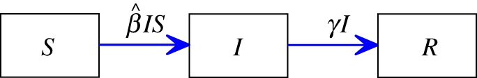
Mass action flow diagram. The flux of individuals from susceptible to infected to recovered for the standard mass action model. Each compartment accumulates and loses probability at the rates given on the arrows. (Online version in colour.)

The dot denotes differentiation in time. An ODE system allows for easy prediction of details such as early growth rates, final sizes and intermediate dynamics. Using S + I + R = 1, we re-express this as

1.1

The product IS measures the proportion of partnerships that are from an infected individual to a susceptible individual.

The MA model often provides a reasonable description of epidemics; however, it has well-recognized flaws, which cause the frequency of infected to susceptible partnerships to vary from IS. We highlight two. It neglects both social heterogeneity, variation in contact rates which can be quite broad [8,9], and partnership duration, implicitly assuming all partnerships are infinitesimally short. Because of these omissions, model predictions can differ from reality. For example, owing to social heterogeneity, early infections tend to have more partnerships [10] and may cause more infections than ‘average’ individuals, enhancing the early spread over that predicted by the MA model [11–15]. When partnership duration is significant, an infected individual may have already infected its partners, reducing its ability to cause new infections. Because of these assumptions, the MA model predicts the same results for a sexually transmitted disease in a completely monogamous population, a population with serial monogamy, and a population with wide variation in contact levels with mean one. Intuitively, we expect these to produce dramatically different epidemics, but no existing mathematical theory allows analytical comparisons.

Over the past 25 years, attempts have been made to eliminate these assumptions without sacrificing analytical tractability. With few exceptions (notably Volz & Meyers [16]), these make an ‘all-or-nothing’ assumption about partnership duration: partnerships are fleeting and never repeated or they never change. With fleeting partnerships, social heterogeneity is introduced by adding multiple risk groups to the MA model: in extreme cases, there are arbitrarily many subgroups (the mean field social heterogeneity model) [2,17–20]. This model is relatively well understood and can be rigorously reduced to a handful of equations. With permanent partnerships, social heterogeneity is introduced through static networks [12–14,21,22]. Static network results typically give the final size but no dynamic information. Some attempts to predict dynamics with static networks use pair approximation techniques [23] relying on approximation of network structures. More rigorous approaches avoid these approximations, but are more difficult [24–27]. Of these, only Volz [24] yields a closed ODE system, (see also [28,29]). This model lacks an illustration like figure 1, hampering communication and further development. Finite, non-zero partnership duration is typically handled through simulation, which is often too slow to effectively study parameter space.

Although no coherent mathematical structure to study social heterogeneity and partnership duration exists, there have been studies collecting these data in real-world contexts [9,10,30,31]. Typically, the resulting measurements have been reduced to average contact rates to make the mathematics tractable. Much of the available and potentially relevant detail is therefore discarded because existing models cannot capture the detail collected.

We find that the appropriate perspective allows us to develop conceptually and mathematically simple models that incorporate social heterogeneity and (arbitrary) partnership duration. This provides a unifying framework for existing models and allows an expanded universe of models. Our goal in each case is to calculate the susceptible, infected or recovered proportions of the population, but we find that this can be answered more easily using an equivalent problem. We ask the question, ‘what is the probability that a randomly chosen test node u is susceptible, infected or recovered?’ Because u is chosen randomly, the probability that u is susceptible equals the proportion susceptible S(t), and similarly for I and R. If we know S(t), then the initial conditions and , I = 1 − S − R determine I(t) and R(t) as in equation (1.1).

The probability that u is susceptible is the probability that no partner has ever transmitted infection to u. The method to calculate this is the focus of this study. This probability depends on how many partners u has, the rate its partners change, and the probability that a random partner is infected at any given time. Because a random partner is likely to have more partners than a random individual, knowing the infected fraction of the population does not give the probability that a partner of u is infected. We focus on the probability that a random partner is infected rather than the probability a random individual is infected. Once we calculate this, it is straightforward to calculate that the probability u is susceptible. The resulting edge-based compartmental modelling approach significantly increases the effects we can study compared with MA models, but with only a small complexity penalty.

In this study, we consider the spread of epidemics in two general classes of networks: actual degree networks (based on configuration model networks [32–34]) and expected degree networks (based on mixed Poisson network; commonly called Chung-Lu networks [35–37]). In both cases, we can consider static and dynamic networks. In actual degree networks, a node is assigned k stubs where k is a random non-negative integer assigned independently for each node from some probability distribution. Edges are created by pairing stubs from different nodes. In expected degree networks, a node is assigned κ, where κ is a random non-negative real number. Edges are assigned between two nodes u and v with probability proportional to κ_uκ_v. We develop exact differential equations for the large population limit, which we compare with simulations. Detailed descriptions of the simulation techniques are given in the electronic supplementary material.

For many assumptions about population structure, the equations we derive are equivalent to those found by others. These previous equations have not been widely used. We speculate that this is because the derivation underlying the earlier equations are not for the faint of heart, and consequently the models have been conceptually difficult as well. The main result of this study is a conceptual shift, after which the derivations become straightforward, and the equations become simpler.

We summarize the populations we consider in table 1. We begin by analysing the simplest edge-based compartmental model in detail, exploring epidemic spread in a static network of known degree distribution, a configuration model (CM) network. To derive the equations, we introduce a flow diagram that leads to a simple mathematical formulation. We next consider disease spreading through dynamic actual degree networks and then static and dynamic expected degree networks. The template shown here allows us to derive a handful of ODEs for each of these populations. Unsurprisingly, the stronger our assumptions, the simpler our formulation becomes. We neglect heterogeneity within the population other than the contact rates, assume that the disease has a very simple structure and assume that the population is at statistical equilibrium prior to disease introduction.

Table 1.

Populations to which we apply edge-based compartmental models.

model	population structure	section
configuration model (CM)	static network with specified degree distribution, assigned using the probability mass function P(k).	2
dynamic fixed-degree (DFD)	dynamic network for which each node's degree remains a constant value, assigned using P(k).	3.2
dormant contact (DC)	dynamic fixed-degree network incorporating gaps between partnerships; a node may wait before replacing a partner.	3.3
mixed Poisson model (MP)	static network with specified distribution of expected degrees κ assigned using the probability density function ρ(κ).	4.1
dynamic variable-degree (DVD)	dynamic network with degrees varying in time with averages assigned using ρ(κ).	4.3
mean field social heterogeneity (MFSH)	population with a distribution of contact rates assigned using P(k) or ρ(κ) and negligible partnership duration.	3.1 and 4.2

2. Configuration model epidemics

We demonstrate our approach with CM networks. A CM network is static with a known degree distribution (the distribution of the number of partners). We create a CM network with N nodes as follows: we assign each node u its degree k_u with probability P(k_u) and give it k_u stubs (half-edges). Once all nodes are assigned stubs, we pair stubs randomly into edges representing partnerships. The probability a randomly selected node u has degree k is P(k). In contrast, the probability a stub of u connects to some stub of v is proportional to k_v. So the probability a randomly selected partner (or neighbour) of u has degree k is

See earlier studies [15,38] for more detail. A sample CM network is shown in figure 2.

Figure 2.

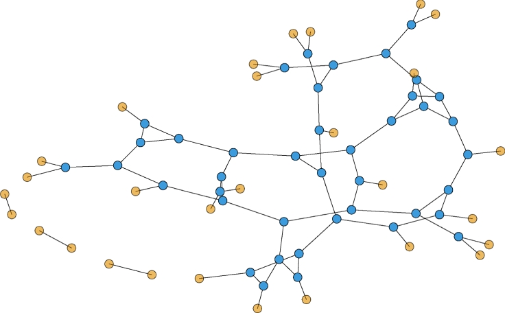
A sample configuration model network. Half the nodes have degree 3 and half degree 1. Partners are chosen randomly. The probability a partner has degree 3 is three times the probability it has degree 1. In general, the probability a partner has degree k is P_n(k) = kP(k)/〈K〉. (Online version in colour.)

We assume that the disease transmits from an infected node to a partner at rate β. If the partner is susceptible, then it becomes infected. Infected nodes recover at rate γ. Throughout, we assume a large population, a small initial proportion infected, a small initial proportion of stubs belonging to infected nodes and a growing outbreak. Our equations become correct once the number of infections NI has grown large enough to behave deterministically, whereas the proportion infected I is still small. Until stochastic effects are unimportant, other methods such as branching process approximations [39] (which apply in large populations with small numbers infected) may be more useful.

To calculate S(t), I(t) and R(t), we note that these are the probabilities that a random test node u is in each state. We calculate S(t) by noting that it is also the probability none of u's partners has yet transmitted to u. We would like to treat each partner as independent, but the probability that one partner v has become infected is affected by whether another partner w of u has transmitted to u as u could infect v. Accounting for this directly requires considerable bookkeeping. A simpler approach removes the correlation by assuming that u causes no infections. This does not alter the state of u: the probabilities we calculate for u will be the proportion of the population in each state under the original assumption that u behaves as any other node, and so this yields an equivalent problem. Further discussion of this modification is given in the electronic supplementary material.

We define θ(t) to be the probability that a randomly chosen partner has not transmitted to u. Initially, θ is close to 1. For large CM networks, partners of u are independent. So given its degree k, u is susceptible at time t with probability s(k,θ(t)) = θ(t)^k. Thus, where

is the probability generating function [40] of the degree distribution (such functions have many useful properties, of which we use three: its derivative is 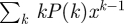, its second derivative is 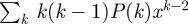and ψ′(1) = 〈K〉). For many important probability distributions, ψ takes a simple form, which simplifies our examples. Combining with the flow diagram for S, I and R in figure 3, we have

Figure 3.

Edge-based compartmental modelling for configuration model (CM) networks. The flow diagram for a static CM network. (a) The ϕ_S, ϕ_I and ϕ_R compartments represent the probability that a partner is susceptible, infected or recovered and has not transmitted infection. The 1 − θ compartment is the probability that it has transmitted. The fluxes between the ϕ compartments result from infection or recovery of a partner of the test node and the ϕ_I to 1 − θ flux results from a partner transmitting infection to the test node. (b) S, I and R represent the proportion of the population susceptible, infected and recovered. We can find S explicitly, and I and R follow as in the mass action model. (Online version in colour.)

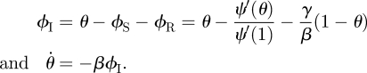
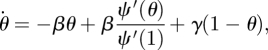
To calculate the new variable θ, we break it into three parts: the probability that a partner v is susceptible at time t, ϕ_S; the probability that v is infected at time t but has not transmitted infection to u, ϕ_I; the probability that v has recovered by time t but did not transmit infection to u, ϕ_R. Then θ = ϕ_S + ϕ_I + ϕ_R. Initially, ϕ_S and θ are approximately 1 while ϕ_I and ϕ_R are small (they sum to θ − ϕ_S). The flow diagram for ϕ_S, ϕ_I, ϕ_R and 1 − θ (figure 3) shows the probability fluxes between these compartments. The rate an infected partner transmits to u is β; so the ϕ_I to 1 − θ flux is βϕ_I. We conclude . To find ϕ_I, we will use ϕ_I = θ− ϕ_S − ϕ_R and calculate ϕ_S and ϕ_R explicitly.

The rate at which an infected partner recovers is γ. Thus the ϕ_I to ϕ_R flux is γϕ_I. This is proportional to the flux into 1 − θ with the constant of proportionality γ/β. As ϕ_R and 1 − θ both begin as approximately 0, we have ϕ_R = γ(1 − θ)/β. To find ϕ_S, recall a partner v has degree k with probability P_n(k) = kP(k)/〈K〉. Given k, v is susceptible with probability θ^k−1 (we disallow transmission from u; so k − 1 nodes can infect v). A weighted average gives

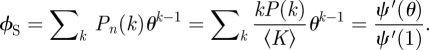Thus

Thus our equations become

2.1

and

2.2

This captures substantially more population structure than the MA model with only marginally more complexity. This is the system of Miller [28] and is equivalent to that of Volz [24]. It improves on approaches of earlier studies [25,26], which require either 𝒪(M) or 𝒪(M²) ODEs, where M is the (possibly unbounded) maximum degree. This derivation is simpler than Volz [24] because we choose variables with a conserved quantity, simplifying the bookkeeping.

The edge-based compartmental modelling approach we have introduced forms the basis of our study. Depending on the network structure, some details will change. However, we will remain as consistent as possible.

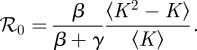
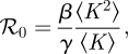
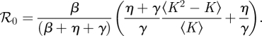
2.1. ℛ₀ and final size

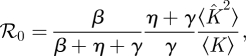
One of the most important parameters for an infectious disease is its basic reproductive number ℛ₀, the average number of infections caused by a node infected early in an epidemic. When ℛ₀ < 1 epidemics are impossible, while when ℛ₀ > 1 they are possible, though not guaranteed. For this model, we find that ℛ₀ is (see the electronic supplementary material)

2.3

We want the expected final size if an epidemic occurs. We set in equation (2.1) and solve

2.4

for θ(∞). If ℛ₀ > 1 then this has two solutions, the larger of which is θ = 1 (the pre-disease equilibrium). We want the smaller solution. The total fraction of the population infected in the course of an epidemic is ℛ(∞) = 1 − ψ(θ(∞)). These calculations of ℛ₀ and ℛ(∞) are in agreement with previous observations [11–13,41,42]. When ℛ₀ < 1, our approach breaks down: full details are given in the electronic supplementary material.

2.2. Example

We consider a disease with β = 0.6 and γ = 1. Figure 4 compares simulations with solutions to our ODEs using four different CM networks, each with 5 × 10⁵ nodes and average degree 〈K〉 = 5, but different degree distributions. In order from latest peak to earliest peak, the networks are: every node has degree 5, the degree distribution is Poisson with mean 5, half the nodes have degree 2 and the other half degree 8 and finally a truncated powerlaw distribution in which P(k) ∝ k^−νe^−k/40, where ν = 1.418. We see that the degree distribution significantly alters the spread, with increased heterogeneity leading to an earlier peak, but generally a smaller epidemic. Our predictions fit, while the MA model using fails.

Figure 4.

Configuration model (CM) example (§2.2). Model predictions (dashed) match simulated epidemics (solid) of the same disease on four CM networks with 〈K 〉 = 5 and 5 × 10⁵ nodes, but different degree distributions. Each solid curve is a single simulation. Time is set so t = 0 when there is 1% cumulative incidence. The corresponding mass action model (short dashes) based on the average degree does not match. (Online version in colour.)

3. Actual degree models

For the CM networks, each node has a specific number of stubs. Edges are created by pairing stubs, and no partner changes occur. In generalizing to dynamic ‘actual degree’ models, we assign each node a number of stubs, but allow edges to break and the freed stubs to create new edges. We consider three limits. In the first, the mean field social heterogeneity (MFSH) model, at every moment a stub is connected to a new partner. In the second, the dynamic fixed-degree (DFD) model, edges last for some time before breaking. When an edge breaks, the stubs immediately form new edges with stubs from other edges that have just broken. In the third, the dormant contact (DC) model, we assume edges break as in the DFD model, but stubs wait before finding new partners.

3.1. Mean field social heterogeneity

For the MFSH model, the number of stubs k an individual has is assigned using the probability mass function P(k). At each moment in time, all stubs are rewired to form new edges. A sample network at two times is shown in figure 5.

Figure 5.

Sample mean field social heterogeneity network. (a) One moment in time and (b) an arbitrarily short time later. Half the nodes have degree 3 and the others degree 1. The degrees remain the same, but the edges are all changed. (Online version in colour.)

We analyse the MFSH model similarly. We take θ as the probability a stub has never transmitted infection to the test node u from any partner. To define ϕ_S, ϕ_I and ϕ_R, we require that the stub has not transmitted infection to u and additionally the current partner is susceptible, infected or recovered. As at each moment an individual chooses a new partner, the probability of connecting to a node of a given status is the proportion of all stubs belonging to nodes of that status. We must track the proportion of stubs that belong to susceptible, infected or recovered nodes π_S, π_I and π_R. Because of the rapid turnover of partners, we find that ϕ_S is the product of the probability that a stub has not transmitted θ with the probability it has just joined with a susceptible partner π_S so ϕ_S = θπ_S. Similarly, ϕ_I = θπ_I and ϕ_R = θπ_R.

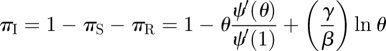
We create flow diagrams as before in figure 6. The S, I and R diagram is unchanged, but the diagram for the ϕ variables and 1 − θ changes. There are no ϕ_S to ϕ_I or ϕ_I to ϕ_R fluxes because of the explicit assumption that the partners associated with a single stub any two times are independent. The change in partner status is owing to ending and forming partnerships rather than infection or recovery of the partner. The flux into 1 − θ from ϕ_I is βϕ_I as before. We need a new flow diagram for π_S, π_I and π_R similar to that for S, I and R. Stubs belonging to infected nodes become stubs belonging to recovered nodes at rate γ, thus . We calculate π_S explicitly: the probability a stub belongs to a node of degree k is P_n(k), and the probability the node is susceptible is θ^k. A weighted average ∑kP_n(k)θ^k gives π_S = θψ′(θ)/ψ′(1). Finally, π_I = 1 − π_S − π_R.

Figure 6.

Mean field social heterogeneity model. The flow diagram for the MFSH model (actual degree formulation). Because partnerships are durationless, partners do not change status while joined to a node; so there is no flux between the ϕ variables (a). The new variables π_S, π_I and π_R (bottom, b) represent the probability that a randomly selected stub belongs to a susceptible, infected or recovered node. We can find π_S in terms of θ and then solve for π_I and π_R in much the same way we solve for I and R in the configuration model. We then find that each ϕ variable is θ times the corresponding π variable. (Online version in colour.)

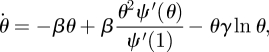
Combining these observations 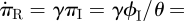. So, π_R = −(γ/β) ln θ (the constant of integration is 0). We have

and . Thus

3.1

and

3.2

The MFSH model has been considered previously [2,17–20], with the population stratified by degree. Setting ζ to be the proportion of all stubs that belong to infected nodes (equivalent to π_I above), the pre-existing system is

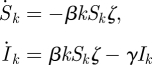where S_k and I_k are the probabilities a random individual with k partners is susceptible or recovered. A known change of variables reduces this to a few equations equivalent to ours.

3.1.1. ℛ₀ and final size

We find

3.3

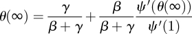
consistent with previous observations [2]. The total proportion infected is R(∞) = 1 − ψ(θ(∞)), where

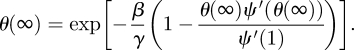3.4

Full details are given in the electronic supplementary material.

3.1.2. Example

We take a population with degrees 1, 5 and 25. The proportions are chosen such that an equal number of stubs belong to each class: P(1) = 25/31, P(5) = 5/31 and P(25) = 1/31. Thus

We set β = γ = 1 and compare a simulation in a population of 5 × 10⁵ with theory in figure 7.

Figure 7.

Mean field social heterogeneity example (§3.1.2). Model predictions (dashed) match a simulated epidemic (solid) in a population of 5 × 10⁵ nodes. The solid curve is a single simulation. Time is set so t = 0 when there is 1% cumulative incidence. The degree distribution satisfies P(1) = 25/31, P(5) = 5/31 and P(25) = 1/31. (Online version in colour.)

3.2. Dynamic fixed-degree

The DFD model interpolates between the CM and MFSH models. We assign each node's degree k as before and pair stubs randomly. As time progresses, edges break. The freed stubs immediately join with stubs from other edges that break, a process we refer to as ‘edge swapping’. The rate an edge breaks is η. A sample network at two times is shown in figure 8.

Figure 8.

Sample dynamic fixed-degree network. (a) One moment in time and (b) a short time later. When edges break, the nodes immediately form new edges with other nodes whose edges break simultaneously. In our simulations, edges break in pairs, but that is not required for the theory. Half of the nodes have degree 3 and the other half have degree 1. (Online version in colour.)

We develop flow diagrams (figure 9) as before. The S, I and R diagram is unchanged. We again track the probabilities π_S, π_I and π_R that a random stub belongs to a susceptible, infected or recovered node, respectively. The diagram is unchanged. The diagram for θ and the ϕ variables changes: we have fluxes from ϕ_S to ϕ_I and ϕ_I to ϕ_R representing infection or recovery of the partner as in the CM model, but we also have fluxes from ϕ_S to ϕ_S, ϕ_I or ϕ_R resulting from edge swapping. We have similar edge swapping fluxes from ϕ_I and ϕ_R. The flux into ϕ_S from edge swapping is ηθπ_S. The flux out of ϕ_S from edge swapping is ηϕ_S. Similar results hold for ϕ_I and ϕ_R.

Figure 9.

Dynamic fixed-degree (DFD) model. The flow diagram for the DFD model. Unlike the configuration model case, we cannot calculate ϕ_S explicitly, so we must calculate the ϕ_S to ϕ_I flux. (Online version in colour.)

Our earlier techniques to find ϕ_I break down. We solve for ϕ_S and ϕ_I using ODEs. To complete the system, we need the ϕ_S to ϕ_I flux. Consider a partner v of our test node u such that: the stub belonging to u never transmitted to u and the stub belonging to v never transmitted to v prior to the u–v edge forming. Given this, the probability v is susceptible is (1). Thus, given that v is susceptible, v becomes infected at rate

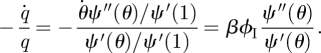Thus the ϕ_S to ϕ_I flux is the product of ϕ_S, the probability that a stub has not transmitted infection to the test node and connects to a susceptible node, with βϕ_Iψ″(θ)/ψ′(θ), the rate the node becomes infected given that the stub has not transmitted and connects to a susceptible node. This completes figure 9.

The model requires more equations, but remains relatively simple:

3.5

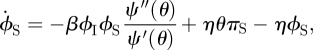3.6

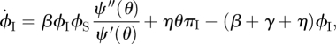3.7

3.8

and

3.9

This is simpler than, but equivalent to, the model of Volz & Meyers [16].

3.2.1. ℛ₀ and final size

We find

3.10

We do not find a simple expression for final size. Instead, we must solve the ODEs numerically. Full details are given in the electronic supplementary material.

3.2.2. Example

We choose a population having negative binomial degree distribution NB(4,1/3) with size parameter r = 4 and probability p = 1/3. Thus . The mean is 2 and the variance 3. For negative binomial distributions, ψ(x) = [(1 − p)/(1 − px)]^r; so

We take β = 5/4, γ = 1 and η = 1/2. The equations accurately predict the spread (figure 10).

Figure 10.

Dynamic fixed-degree example (§3.2.2). Model predictions (dashed) match the average of 102 simulated epidemics (solid) in a population of 10⁴ nodes. For each simulation, time is chosen so that t = 0 corresponds to 3% cumulative incidence. Then, they are averaged to give the solid curve. The degree distribution satisfies for r = 4, p = 1/3. (Online version in colour.)

Our simulations are slower because we must track edges; so we have used smaller population sizes. To reduce noise, we perform 250 simulations, averaging the 102 that become epidemics.

3.3. Dormant contacts

We finally generalize the DFD model, allowing stubs to enter a dormant phase after edges break. This is the most general model we present. It reduces to any model of this study in appropriate limits [43]. It is appropriate for serial monogomy where individuals to not immediately find a new partner.

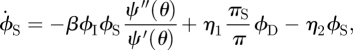
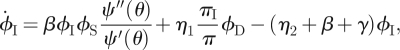
A node is assigned k_m stubs using the probability mass function P(k_m). We take . A stub is dormant or active depending on whether it is currently connected to a partner. The maximum degree of a node is k_m and the ‘active’ and ‘dormant’ degrees are k_a and k_d, respectively, k_a + k_d = k_m. In addition to ϕ_S, ϕ_I and ϕ_R, we add ϕ_D denoting the probability that a stub is dormant and has never transmitted infection from a partner; so θ = ϕ_S + ϕ_I + ϕ_R + ϕ_D. Active stubs become dormant at rate η₂ and dormant stubs become active at rate η₁. A sample network at two times is shown in figure 11.

Figure 11.

Sample dormant contact network. (a) One moment in time and (b) a short time later. Half the nodes have five stubs and the other half have two stubs. When edges break, the stubs become dormant. Dormant stubs can join together to form edges. (Online version in colour.)

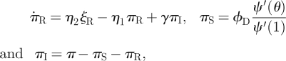
We now develop flow diagrams (figure 12). The diagram for S, I and R is as before. The diagram for θ and the ϕ variables is similar to the DFD model, but with the new compartment ϕ_D. The fluxes associated with edge breaking are at rate η₂ times ϕ_S, ϕ_I or ϕ_R and go from the appropriate compartment into ϕ_D, for a total of η₂(θ − ϕ_D). To describe fluxes owing to edge creation, we generalize the definitions of π_S, π_I and π_R to give the probability that a stub is dormant (and thus available to form a new partnership) and belongs to a susceptible, infected or recovered node, with π = π_S + π_I + π_R the probability a stub is dormant. The probability that a new partner is susceptible, infected or recovered is π_S/π, π_I/π and π_R/π, respectively. The fluxes associated with edge creation occur at total rate η₁ϕ_D, with proportions π_S/π, π_I/π and π_R/π into ϕ_S, ϕ_I and ϕ_R, respectively.

Figure 12.

Dormant contact model. A flow diagram accounting for the dormant stage. (a) Movement of stubs between different stages, including dormant. Stubs are classified by whether they have received infection and the status (or existence) of the current partner. (b) The flow of individuals between different states. (c) Movement of stubs between states with stubs classified based on the status of the node to which they belong. (Online version in colour.)

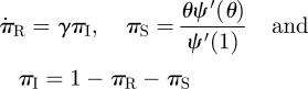
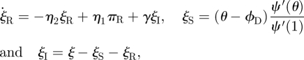
The flow diagram for the π variables is related to that for the DFD model, but we must account for active and dormant stubs. We use ξ_S, ξ_I and ξ_R to be the probabilities that a stub is active and belongs to each type of node, with 1 − π = ξ =ξ_S + ξ_I + ξ_R the probability that a stub is active. The π_S to ξ_S and ξ_S to π_S fluxes are η₁π_S and η₂ξ_S, respectively. Similar results hold for the other compartments. We can use this to show from which we can conclude that (at equilibrium) π = η₂/(η₁ + η₂) and ξ = η₁/(η₁ + η₂). The fluxes from ξ_I and π_I to ξ_R and π_R, respectively, represent recovery of the node the stub belongs to and so are γξ_I and γπ_I, respectively.

We can calculate ξ_S and π_S explicitly. The probability a dormant stub belongs to a susceptible node is π_S = ϕ_Dψ′(θ)/ψ′(1), where ϕ_D is the probability the dormant stub has never received infection, and ψ′(θ)/ψ′(1) is the probability that none of the other stubs have received infection. Similarly, the probability that an active stub belongs to a susceptible node is ξ_S = (θ − ϕ_D)ψ′(θ)/ψ′(1). We can use π_I = π− π_S − π_R and ξ_I = ξ− ξ_S − ξ_R to simplify the system further.

Our new equations are

3.11

3.12

3.13

3.14

3.15

3.16

3.17

and

3.18

3.3.1. ℛ₀ and final size

We can show that

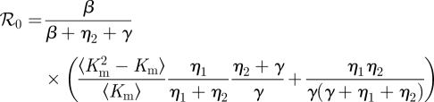3.19

However, we have not found a simple final size relation. Details are given in the electronic supplementary material.

3.3.2. Example

In figure 13, we consider the spread of a disease through a network with dormant edges. The distribution of k_m is Poisson with mean 3

Figure 13.

Dormant contact example (§3.3.2). The average of 155 simulated epidemics in a population of 5000 nodes (solid) with a Poisson maximum degree distribution of mean 3 compared with theory (dashed). Simulations are shifted in time so that t = 0 corresponds to 3% cumulative incidence and then averaged. Because stochastic effects are not negligible, the individual peaks are not perfectly aligned, so the averaging has a small, but noticeable, effect to reduce and broaden the simulated peak. As population size increases, this disappears. (Online version in colour.)

The parameters are β = 2, γ = 1, η₁ = γ and η₂ = γ/2. Simulations are again slow; so we use a smaller population with 322 simulations, and average the 155 that become epidemics.

4. Expected degree models

We now consider SIR diseases spreading through ‘expected degree’ networks. In these networks, each individual has an expected degree κ, which need not be an integer. It is assigned using the probability density function ρ(κ). Edges are placed between two nodes with probability proportional to the expected degrees of the two nodes. In the actual degree models, once a stub belonging to u was joined into an edge, it became unavailable for other edges: the existence of a u–v edge reduced the ability of u to form other edges. In contrast, for expected degree models, edges are assigned independently: a u–v edge does not affect whether u forms other edges. Similar to actual degree models, a partner will tend to have larger expected degree than a randomly chosen node. The probability density function for a partner to have expected degree κ is ρ_n(κ) = κρ(κ)/〈K〉.

Our approach remains similar. We consider a randomly chosen test node u which cannot infect its partners, and calculate the probability that u is susceptible. We first consider the spread of disease through static ‘mixed Poisson’ (MP) networks (also called Chung-Lu networks), for which an edge from u to v exists with probability κ_uκ_v/(N − 1)〈K〉. We then consider the expected degree formulation of MFSH. Following this, we consider the more general dynamic variable-degree (DVD) model, for which a node creates and deletes edges as independent events, unlike the DFD model where deleted edges were instantly replaced. The MP model produces equations effectively identical to the CM equations. The MFSH equations differ somewhat from the actual degree version, but may be shown to be formally equivalent [43]. The DVD equations are simpler than the DFD equations, and it may be more realistic because it does not enforce constant degree for an individual.

4.1. Mixed Poisson

We now consider the MP model. In this model, each node is assigned an expected degree κ using the probability density function ρ(κ). A u–v edge exists with probability κ_uκ_v/(N − 1)〈K〉 independently of other edges. We use the name ‘MP’ because at large N the actual degree of nodes with expected degree κ is chosen from a Poisson distribution with mean κ. The degree distribution is a mixture of Poisson distributions. An example is shown in figure 14.

Figure 14.

Sample mixed Poisson model network. Half the nodes have expected degree 3 and the other half 1.5. An edge is assigned between two nodes with probability proportional to the product of their expected degrees. (Online version in colour.)

Consider two nodes u and v whose expected degrees are κ_u and κ_v = κ_u + Δκ with Δκ ≪ 1. Our question is, how much does the additional Δκ reduce the probability that v is susceptible? At leading order, it contributes an extra edge to v with probability Δκ, and we may assume it contributes at most one additional edge. We define Θ to be the probability that an edge has not transmitted infection. With probability ΘΔκ there is an additional edge that has not transmitted. The probability the extra Δκ either does not contribute an edge or contributes an edge that has not transmitted is 1 − Δκ + ΘΔκ = 1 − (1 − Θ)Δκ. If s(κ,t) is the probability that a node of expected degree κ is susceptible, then we have s(κ + Δκ, t) = s(κ, t)[1 − (1 − Θ)Δκ]. Taking Δκ → 0, this becomes ∂s/∂κ =−(1 − Θ)s. Thus, s(κ,t) = exp[−κ(1 − Θ)] and S(t) = Ψ(Θ(t)), where

Note that this is the Laplace transform of ρ evaluated at 1−x. As before, figure 15 gives

and we need Θ(t).

Figure 15.

Mixed Poisson (MP) model. (a) The flux of edges for a static MP network. (b) The flux of individuals through the different stages. (Online version in colour.)

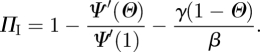
We follow the CM approach almost exactly. The value of Θ is the probability that an edge has not transmitted to the test node u. We define Φ_S, Φ_I and Φ_R to be the probabilities that an edge has not transmitted to u and connects to a susceptible, infected or recovered node; so Θ = Φ_S + Φ_I + Φ_R. To calculate Φ_S, we observe that a partner v of u with expected degree κ has the same probability of having an edge to any w ≠ u as any other node of expected degree κ because edges are created independently of one another. Thus given κ, v is susceptible with probability s(κ,t). Taking the weighted average over all κ gives Φ_S = ∫₀^∞ρ_n(κ)s(κ,t)dt = ∫₀^∞κ exp[−κ(1 − Θ)]ρ(κ)dκ/〈K〉 = Ψ′(Θ)/Ψ′(1). The same techniques as for the CM networks give Φ_R = γ(1 − Θ)/β. Our equations are

This is almost identical to CM epidemics except that Ψ and Θ replace ψ and θ . This similarity is explained in [43].

4.1.1. ℛ₀ and final size

We find

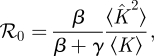where is the average of κ² (which equals the average of k² − k) and 〈K〉 is the average of κ (which equals the average of k). The total proportion infected by an epidemic is R(∞) = 1 − Ψ(Θ(∞)), where

Full details are given in the electronic supplementary material.

4.1.2. Example

We consider a population whose distribution of expected degrees satisfies

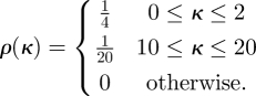Half the individuals have an expected degree between 0 and 2 uniformly, and the other half have expected degree between 10 and 20 uniformly. This gives

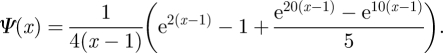We take β = 0.15 and γ = 1, and perform simulations with a population of size 5 × 10⁵ generated using the 𝒪(N) algorithm of Miller & Hagberg [44]. We compare simulation and prediction in figure 16.

Figure 16.

Mixed Poisson (MP) example (§4.1.2). Model predictions (dashed) match a simulated epidemic (solid) in a MP network with 5 × 10⁵ nodes. The solid curve is a single simulation. Time is chosen so that t = 0 corresponds to 1% cumulative incidence. With probability 0.5, expected degrees are chosen uniformly from [0,2], and with probability 0.5 they are chosen uniformly from [10,20]. (Online version in colour.)

4.2. Mean field social heterogeneity

For the expected degree formulation of the MFSH model, the probability that an edge exists between u and v at time t is κ_uκ_v/(N − 1)〈K〉. Whether this edge exists at one moment is independent of whether it exists at any other moment and what other edges exist. A sample network at two times is shown in figure 17.

Figure 17.

Sample mean field social heterogeneity network. (a) One moment in time and (b) an arbitrarily short time later. Half the nodes have expected degree 4 and the others expected degree 1. All edges change, and the actual degree varies with time. (Online version in colour.)

As before, we consider two nodes whose expected degrees differ by Δκ and ask how much the additional Δκ reduces the probability of being susceptible. The definition of Θ is slightly more problematic here because having an edge at one moment is independent of having one later. So it does not make sense to discuss the probability that an edge did not transmit previously because the edge did not exist previously. Instead, we note that in the MP case, (1 − Θ)Δκ could be interpreted as the probability that the additional amount of Δκ ever contributed an edge that had transmitted infection. Guided by this, we define Θ so that as Δκ → 0, the extra amount of Δκ has at some time contributed an edge that transmitted to the node with probability (1 − Θ)Δκ. This again leads to

The flow diagram for S, I and R (figure 18) is unchanged:

Figure 18.

Mean field social heterogeneity (MFSH) model. The flow diagram for a MFSH population (expected degree formulation). This is similar to the actual degree formulation in figure 6. The new variables Π_S, Π_I and Π_R (bottom, b) represent the probability that a newly formed edge connects to a susceptible, infected or recovered node; they can be thought of as the relative rates at which each group forms edges. As the test node does not cause infections, and the probability that a partnership is with a node of a given κ is equal to the probability that a new partner will be with a node of the given κ, the probability that a current partner has a given state is equal to the probability that a new partner has that state. Thus each Φ variable equals the corresponding Π variable. (Online version in colour.)

To find the evolution of Θ, we define Φ_S, Φ_I and Φ_R to be the probabilities that a current edge connects u to a susceptible, infected or recovered node, respectively. The probability that a small extra amount Δκ currently contributes an edge and previously had a different edge that transmitted scales like Δκ²(1 − Θ). As Δκ² ≪ Δκ, this is negligible compared with the probability that there is a current edge. We conclude that at leading order, Φ_SΔκ , Φ_IΔκ and Φ_RΔκ give the probability that the Δκ contributes a current edge connected to a susceptible, infected or recovered node and there has never been a transmission owing to this extra Δκ.

We can construct a flow diagram between Φ_S Δκ , Φ_IΔκ, Φ_RΔκ and (1 − Θ)Δκ. Because all of these have Δκ in them, we factor it out to just use Φ_S, Φ_I, Φ_R and 1 − Θ. Because edges have no duration, there is no Φ_S to Φ_I or Φ_I to Φ_R flux. Instead, there is flux in and out of these compartments representing the continuing change of edges. The Φ_I to 1 − Θ flux is βΦ_I.

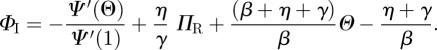
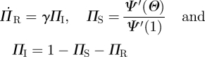
Because edges have no duration, the probability that an edge connects to an individual of a given type is the probability a new edge connects to an individual of that type: Φ_S = Π_S , Φ_I = Π_I and Φ_R = Π_R where Π_S, Π_I and Π_R are the probabilities that a newly formed edge connects to a susceptible, infected or recovered node, respectively.¹ We have Π_S = Ψ′(Θ)/Ψ′(1) and . As Π_I = Φ_I, this means 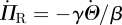. Integrating gives Π_R = γ (1 − Θ)/β. So

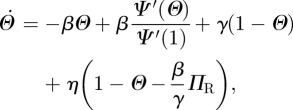
Since 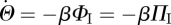, finally, we have

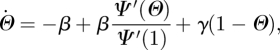and

Under appropriate limits, the MFSH equations in k reduce to those in κ and vice versa; so the models are equivalent [43]. Surprisingly, this system differs from the MP equations only in the first term of the equation.

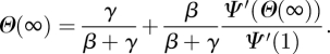
4.2.1. ℛ₀ and final size

We find

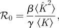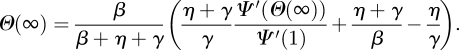
and the final size is R(∞) = 1 − Ψ(Θ(∞)), where Θ(∞) solves

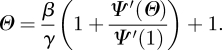Full details are given in the electronic supplementary material.

4.2.2. Example

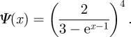
For our example, we take a population with ρ(κ) = e^κ/(e³ − 1) for 0 < κ< 3 and 0 otherwise, giving

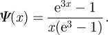We take γ = 1 and β = 0.435 and compare simulation with theory in figure 19. We choose these parameters to demonstrate that the approach remains accurate for small ℛ₀ = 1.04. We use a population of 15 × 10⁶. There is noise as the epidemic does not infect a large number of people.

Figure 19.

Expected degree mean field social heterogeneity (MFSH) example (§4.2.2). Model predictions (dashed) match a simulated epidemic (solid) in a MFSH network with 15 × 10⁶ nodes. The solid curve is a single simulation. Time is chosen so that t = 0 corresponds to 0.5% cumulative incidence. Expected degrees are chosen with ρ(κ) = e^κ/(e³−1) for 0<κ<3. (Online version in colour.)

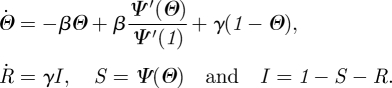
4.3. Dynamic variable-degree

The DVD model interpolates between the MP model and the expected degree formulation of the MFSH model. Each node is assigned κ using ρ(κ) and creates edges at rate κη (joining to another node also creating an edge). Existing edges break at rate η. Thus, a node has expected degree κ, though its value varies around κ. In fact, it is Poisson-distributed over time. A sample network at two times is shown in figure 20.

Figure 20.

Sample dynamic variable-degree network. (a) One moment in time and (b) a short time later. The formation or deletion of an edge has no impact on other edges. Half the nodes have expected degree 4 and the other half 1. (Online version in colour.)

We define Θ such that the probability that a small Δκ has ever contributed an edge that has transmitted infection is (1 − Θ)Δκ . We again have

We generalize the earlier definitions and define Φ_S, Φ_I and Φ_R to be the probabilities a current edge has never transmitted infection and connects to a susceptible, infected or recovered node.

We define Π_S, Π_I and Π_R to be the probabilities a new edge connects to a susceptible, infected or recovered node. We have Π_S = Ψ′(Θ)/Ψ′(1), Π_I = 1 − Π_S − Π_R and . We build the flow diagram for Φ_SΔκ, Φ_IΔκ, Φ_RΔκ and (1 − Θ)Δκ. There is flux into Φ_SΔκ at rate ηΠ_SΔκ because this is the rate at which the Δκ leads to edge creation. There is flux out of Φ_SΔκ at rate ηΦ_SΔκ because existing edges break at rate η, and the probability that such an edge exists is Φ_SΔκ. Similar fluxes exist for Φ_I and Φ_R. The flux out of Φ_IΔκ into Φ_RΔκ is γΦ_IΔκ as before, and the flux into (1 − Θ)Δκ is βΦ_IΔκ. We factor out Δκ and the flow diagrams (figure 21) are defined.

Figure 21.

Dynamic variable-degree (DVD) model. The flow diagrams for the DVD model. (Online version in colour.)

Because the existence of an edge from the test node u to the partner v has no impact on any other edges v might have, the partners v has—aside from u—are indistinguishable from the partners of another node with the same κ, and so they are susceptible with the same probability: Φ_S = Π_S. The fluxes into and out of Φ_S from edge creation–deletion balance, and the Φ_S to Φ_I flux is simply . Using this and the other fluxes for Φ_I, we conclude . As and , we can integrate this and find

So can be written in terms of Θ and Π_R. We arrive at

4.1

4.2

and

4.3

This is simpler than the DFD case because the arbitrary smallness of Δκ allowed us to assume that no previous transmission occurred for the Δκ, whereas for a discrete stub, we cannot neglect previous transmission.

4.3.1. ℛ₀ and final size

We find

The total proportion infected is R(∞) = 1 − Ψ(Θ(∞)), where

Full details are given in the electronic supplementary material.

4.3.2. Example

We choose the same distribution of κ as of k in the DFD example, NB(4,1/3). We find

We take the same parameters β = 5/4, γ = 1 and η = 1/2. Figure 22 shows that the equations accurately predict the spread. As in the DFD and DC case, we use an average as the comparison point, taking 240 simulations and averaging the 92 resulting in epidemics.

Figure 22.

Dynamic variable-degree example (§4.3.2). Model predictions (dashed) match the average of 92 simulated epidemics (solid) in a population of 10⁴ nodes. For each simulation, time is chosen so that t = 0 corresponds to 3% cumulative incidence. Then, they are averaged to give the solid curve. κ is chosen from the same distribution as k in figure 10. (Online version in colour.)

The final size is larger than for the DFD model. Although the average numbers of partners are all the same, the increase in transmission routes when an individual has more partners than expected outweighs the decrease when the number is less than expected. The net effect is to increase the final size.

5. Discussion

We have introduced a new approach to study the spread of infectious diseases. This edge-based compartmental modelling approach allows us to simultaneously consider the impacts of partnership duration and social heterogeneity. It is conceptually simple and leads to equations of comparable simplicity to the MA model. It produces a broad family of models that contains several known models as special cases. It further allows us to investigate the effect of many behaviours that have previously been inaccessible to analytical study.

A significant contribution of this work is that it allows us to study the spread of a disease in a population for which some individuals have different propensity to form partnerships while allowing us to explicitly incorporate the impact of partnership duration. The interaction of partnership duration and numbers of overlapping partnerships plays a significant role in the spread of many diseases, and in particular may play an important role in the spread of HIV [45]. These techniques open the door to studying these questions analytically rather than relying on simulation.

The edge-based compartmental modelling approach has a simple, graphical interpretation through flow diagrams. This simplifies model description, and guides generalizations. We propose that this is the correct perspective to study the deterministic dynamics of SIR epidemics on random networks because the derivations are straightforward, we need to track only a small number of compartments and we do not require any closure approximations. Other existing techniques rely on approximations [23] or produce complicated or large systems of equations [24–26]. This approach does not offer immediate insight into stochastic effects where methods such as branching processes are more appropriate. In later studies, we use this approach to derive other generalizations, including different correlations in population structure, different disease dynamics and populations that change structure in response to the spreading disease.

Our approach is limited by the assumption that infection of one partner of u can be treated as independent of that of another partner. This is a strong assumption, and prevents us from applying this model to susceptible–infected–susceptible (SIS) diseases for which individuals return to a susceptible state. In this case, the assumption that u does not infect its partners can alter the future state of u. In the real population, if u becomes infected, it can infect partners who then infect u when u returns to a susceptible state. Thus if partnership duration is nonzero, our predictions may be significantly altered. This limitation is often not recognized but may lead to important failures of mean-field or MA models when applied to a population for which partnership duration is important [46].

Treating partners as independent also means that if v and w are partners of u, we assume no alternate short path between v and w exists. In particular, we assume that clustering [47,48] is negligible: partners are unlikely to see one another. This assumption applies equally to most existing analytical epidemic models, but it can be eliminated in very special cases using techniques similar to those of earlier studies [49–52].

References

- 1.Kermack W. O., McKendrick A. G. 1927. A contribution to the mathematical theory of epidemics. Proc. R. Soc. Lond. A 115, 700–721 10.1098/rspa.1927.0118 (doi:10.1098/rspa.1927.0118) [DOI] [Google Scholar]
- 2.Anderson R. M., May R. M. 1991. Infectious diseases of humans. Oxford, UK: Oxford University Press [Google Scholar]
- 3.Lloyd A. L., May R. M. 2001. How viruses spread among computers and people. Science 292, 1316–1317 10.1126/science.1061076 (doi:10.1126/science.1061076) [DOI] [PubMed] [Google Scholar]
- 4.Kiss I. Z., Green D. M., Kao R. R. 2006. The network of sheep movements within Great Britain: network properties and their implications for infectious disease spread. J. R. Soc. Interface 3, 669–677 10.1098/rsif.2006.0129 (doi:10.1098/rsif.2006.0129) [DOI] [PMC free article] [PubMed] [Google Scholar]
- 5.Rohani P., Zhong X., King A. A. 2010. Contact network structure explains the changing epidemiology of pertussis. Science 330, 982–985 10.1126/science.1194134 (doi:10.1126/science.1194134) [DOI] [PubMed] [Google Scholar]
- 6.Eubank S., Guclu H., Anil Kumar V. S., Marathe M. V., Srinivasan A., Toroczkai Z., Wang N. 2004. Modelling disease outbreaks in realistic urban social networks. Nature 429, 180–184 10.1038/nature02541 (doi:10.1038/nature02541) [DOI] [PubMed] [Google Scholar]
- 7.Germann T. C., Kadau K., Longini I. M., Jr, Macken C. A. 2006. Mitigation strategies for pandemic influenza in the United States. Proc. Natl Acad. Sci. USA 103, 5935–5940 10.1073/pnas.0601266103 (doi:10.1073/pnas.0601266103) [DOI] [PMC free article] [PubMed] [Google Scholar]
- 8.Liljeros F., Edling C. R., Amaral L. A. N., Stanley H. E., Åberg Y. 2001. The web of human sexual contacts. Nature 411, 907–908 10.1038/35082140 (doi:10.1038/35082140) [DOI] [PubMed] [Google Scholar]
- 9.Mossong J., et al. 2008. Social contacts and mixing patterns relevant to the spread of infectious diseases. PLoS Med. 5, 381–391 10.1371/journal.pmed.0050074 (doi:10.1371/journal.pmed.0050074) [DOI] [PMC free article] [PubMed] [Google Scholar]
- 10.Christakis N. A., Fowler J. H. 2010. Social network sensors for early detection of contagious outbreaks. PLoS ONE 5, e12948. 10.1371/journal.pone.0012948 (doi:10.1371/journal.pone.0012948) [DOI] [PMC free article] [PubMed] [Google Scholar]
- 11.Andersson H. 1997. Epidemics in a population with social structures. Math. Biosci. 140, 79–84 10.1016/S0025-5564(96)00129-0 (doi:10.1016/S0025-5564(96)00129-0) [DOI] [PubMed] [Google Scholar]
- 12.Newman M. E. J. 2002. Spread of epidemic disease on networks. Phys. Rev. E 66, 016128. 10.1103/PhysRevE.66.016128 (doi:10.1103/PhysRevE.66.016128) [DOI] [PubMed] [Google Scholar]
- 13.Miller J. C. 2007. Epidemic size and probability in populations with heterogeneous infectivity and susceptibility. Phys. Rev. E 76, 010101. 10.1103/PhysRevE.76.010101 (doi:10.1103/PhysRevE.76.010101) [DOI] [PubMed] [Google Scholar]
- 14.Kenah E., Robins J. M. 2007. Second look at the spread of epidemics on networks. Phys. Rev. E 76, 036113. 10.1103/PhysRevE.76.036113 (doi:10.1103/PhysRevE.76.036113) [DOI] [PMC free article] [PubMed] [Google Scholar]
- 15.Meyers L. A., Pourbohloul B., Newman M. E. J., Skowronski D. M., Brunham R. C. 2005. Network theory and SARS: predicting outbreak diversity. J. Theor. Biol. 232, 71–81 10.1016/j.jtbi.2004.07.026 (doi:10.1016/j.jtbi.2004.07.026) [DOI] [PMC free article] [PubMed] [Google Scholar]
- 16.Volz E. M., Meyers L. A. 2007. Susceptible–infected–recovered epidemics in dynamic contact networks. Proc. R. Soc. B 274, 2925–2933 10.1098/rspb.2007.1159 (doi:10.1098/rspb.2007.1159) [DOI] [PMC free article] [PubMed] [Google Scholar]
- 17.May R. M., Anderson R. M. 1988. The transmission dynamics of human immunodeficiency virus (HIV). Phil. Trans. R. Soc. Lond. B 321, 565–607 10.1098/rstb.1988.0108 (doi:10.1098/rstb.1988.0108) [DOI] [PubMed] [Google Scholar]
- 18.May R. M., Lloyd A. L. 2001. Infection dynamics on scale-free networks. Phys. Rev. E 64, 066112. 10.1103/PhysRevE.64.066112 (doi:10.1103/PhysRevE.64.066112) [DOI] [PubMed] [Google Scholar]
- 19.Moreno Y., Pastor-Satorras R., Vespignani A. 2002. Epidemic outbreaks in complex heterogeneous networks. Eur. Phys. J. B 26, 521–529 10.1140/epjb/e20020122 (doi:10.1140/epjb/e20020122) [DOI] [PubMed] [Google Scholar]
- 20.Pastor-Satorras R., Vespignani A. 2001. Epidemic spreading in scale-free networks. Phys. Rev. Lett. 86, 3200–3203 10.1103/PhysRevLett.86.3200 (doi:10.1103/PhysRevLett.86.3200) [DOI] [PubMed] [Google Scholar]
- 21.Diekmann O., De Jong M. C. M., Metz J. A. J. 1998. A deterministic epidemic model taking account of repeated contacts between the same individuals. J. Appl. Probab. 35, 448–462 10.1239/jap/1032192860 (doi:10.1239/jap/1032192860) [DOI] [Google Scholar]
- 22.Andersson H. 1999. Epidemic models and social networks. Math. Sci. 24, 128–147 [Google Scholar]
- 23.Eames K. T. D., Keeling M. J. 2002. Modeling dynamic and network heterogeneities in the spread of sexually transmitted diseases. Proc. Natl Acad. Sci. USA 99, 13 330–13 335 10.1073/pnas.202244299 (doi:10.1073/pnas.202244299) [DOI] [PMC free article] [PubMed] [Google Scholar]
- 24.Volz E. M. 2008. SIR dynamics in random networks with heterogeneous connectivity. J. Math. Biol. 56, 293–310 10.1007/s00285-007-0116-4 (doi:10.1007/s00285-007-0116-4) [DOI] [PMC free article] [PubMed] [Google Scholar]
- 25.Lindquist J., Ma J., van den Driessche P., Willeboordse F. H. 2010. Effective degree network disease models. J. Math. Biol. 62, 143–164 10.1007/s00285-010-0331-2 (doi:10.1007/s00285-010-0331-2) [DOI] [PubMed] [Google Scholar]
- 26.Ball F., Neal P. 2008. Network epidemic models with two levels of mixing. Math. Biosci. 212, 69–87 10.1016/j.mbs.2008.01.001 (doi:10.1016/j.mbs.2008.01.001) [DOI] [PubMed] [Google Scholar]
- 27.Noël P.-A., Davoudi B., Brunham R. C., Dubé L. J., Pourbohloul B. 2009. Time evolution of disease spread on finite and infinite networks. Phys. Rev. E 79, 026101. 10.1103/PhysRevE.79.026101 (doi:10.1103/PhysRevE.79.026101) [DOI] [PubMed] [Google Scholar]
- 28.Miller J. C. 2011. A note on a paper by Erik Volz: SIR dynamics in random networks. J. Math. Biol. 62, 349–358 [DOI] [PubMed] [Google Scholar]
- 29.House T., Keeling M. J. 2010. Insights from unifying modern approximations to infections on networks. J. R. Soc. Interface 8, 67–73 10.1098/rsif.2010.0179 (doi:10.1098/rsif.2010.0179) [DOI] [PMC free article] [PubMed] [Google Scholar]
- 30.Wallinga J., Teunis P., Kretzschmar M. 2006. Using data on social contacts to estimate age-specific transmission parameters for respiratory-spread infectious agents. Am. J. Epidemiol. 164, 936. 10.1093/aje/kwj317 (doi:10.1093/aje/kwj317) [DOI] [PubMed] [Google Scholar]
- 31.Salathé M., Kazandjiev M., Lee J. W., Levis P., Feldman M. W., Jones J. H. 2010. A high-resolution human contact network for infectious disease transmission. Proc. Natl Acad. Sci. USA 107, 22 020–22 025 10.1073/pnas.1009094108 (doi:10.1073/pnas.1009094108) [DOI] [PMC free article] [PubMed] [Google Scholar]
- 32.Molloy M., Reed B. 1995. A critical point for random graphs with a given degree sequence. Random Struct. Algorithms 6, 161–179 10.1002/rsa.3240060204 (doi:10.1002/rsa.3240060204) [DOI] [Google Scholar]
- 33.Newman M. E. J., Strogatz S. H., Watts D. J. 2001. Random graphs with arbitrary degree distributions and their applications. Phys. Rev. E 64, 026118. 10.1103/PhysRevE.64.026118 (doi:10.1103/PhysRevE.64.026118) [DOI] [PubMed] [Google Scholar]
- 34.van der Hofstad R. 2010. Random graphs and complex networks. Eindhoven, The Netherlands: Eindhoven University of Technology [Google Scholar]
- 35.Chung F., Lu L. 2002. Connected components in random graphs with given expected degree sequences. Ann. Comb. 6, 125–145 10.1007/PL00012580 (doi:10.1007/PL00012580) [DOI] [Google Scholar]
- 36.Norros I., Reittu H. On a conditionally Poissonian graph process. Adv. Appl. Probab. 38, 59–75 10.1239/aap/1143936140 (doi:10.1239/aap/1143936140) [DOI] [Google Scholar]
- 37.Britton T., Deijfen M., Martin-Löf A. 2006. Generating simple random graphs with prescribed degree distribution. J. Stat. Phys. 124, 1377–1397 10.1007/s10955-006-9168-x (doi:10.1007/s10955-006-9168-x) [DOI] [Google Scholar]
- 38.Feld S. L. 1991. Why your friends have more friends than you do. Am. J. Sociol. 96, 1464–1477 10.1086/229693 (doi:10.1086/229693) [DOI] [Google Scholar]
- 39.Diekmann O., Heesterbeek J. A. P. 2000. Mathematical epidemiology of infectious diseases. London, UK: Wiley Chichester [Google Scholar]
- 40.Wilf H. S. 2005. Generatingfunctionology, 3rd edn Natick, MA: AK Peters Ltd [Google Scholar]
- 41.Andersson H. 1998. Limit theorems for a random graph epidemic model. Ann. Appl. Probab. 8, 1331–1349 10.1214/aoap/1028903384 (doi:10.1214/aoap/1028903384) [DOI] [Google Scholar]
- 42.Trapman P. 2007. On analytical approaches to epidemics on networks. Theor. Popul. Biol. 71, 160–173 10.1016/j.tpb.2006.11.002 (doi:10.1016/j.tpb.2006.11.002) [DOI] [PubMed] [Google Scholar]
- 43.Miller J. C., Volz E. M. Submitted Model hierarchies in edge-based compartmental modeling for infectious disease spread. [DOI] [PMC free article] [PubMed] [Google Scholar]
- 44.Miller J. C., Hagberg A. 2011. Efficient generation of networks with given expected degrees. In Proc. Algorithms and Models for the Web Graph—8th International Workshop, ‘WAW 2011’, Atlanta, GA, USA, 27–29 May 2011. Lecture Notes in Computer Science (eds M. Frieze, P. Horn, P. Pralat), vol. 6732, pp. 115–126. Berlin, Germany: Springer [Google Scholar]
- 45.Morris M., Kretzschmar M. 1995. Concurrent partnerships and transmission dynamics in networks. Soc. Networks 17, 299–318 10.1016/0378-8733(95)00268-S (doi:10.1016/0378-8733(95)00268-S) [DOI] [Google Scholar]
- 46.Chatterjee S., Durrett R. 2009. Contact processes on random graphs with power law degree distributions have critical value 0. Ann. Probab. 37, 2332–2356 10.1214/09-AOP471 (doi:10.1214/09-AOP471) [DOI] [Google Scholar]
- 47.Watts D. J., Strogatz S. H. 1998. Collective dynamics of ‘small-world’ networks. Nature 393, 409–410 10.1038/30918 (doi:10.1038/30918) [DOI] [PubMed] [Google Scholar]
- 48.Newman M. E. J. Properties of highly clustered networks. Phys. Rev. E 68, 026121. 10.1103/PhysRevE.68.026121 (doi:10.1103/PhysRevE.68.026121) [DOI] [PubMed] [Google Scholar]
- 49.Volz E. M., Miller J. C., Galvani A., Meyers L. A. 2011. The effects of heterogeneous and clustered contact patterns on infectious disease dynamics. PLoS Comput. Biol. 7, e1002042. 10.1371/journal.pcbi.1002042 (doi:10.1371/journal.pcbi.1002042) [DOI] [PMC free article] [PubMed] [Google Scholar]
- 50.Miller J. C. 2009. Percolation and epidemics in random clustered networks. Phys. Rev. E 103, 020901(R). 10.1103/PhysRevE.80.020901 (doi:10.1103/PhysRevE.80.020901) [DOI] [PubMed] [Google Scholar]
- 51.Newman M. E. J. 2009. Random graphs with clustering. Phys. Rev. Lett. 103, 058701. 10.1103/PhysRevLett.103.058701 (doi:10.1103/PhysRevLett.103.058701) [DOI] [PubMed] [Google Scholar]
- 52.Karrer B., Newman M. E. J. 2010. Random graphs containing arbitrary distributions of subgraphs. Phys. Rev. E 82, 066118. 10.1103/PhysRevE.82.066118 (doi:10.1103/PhysRevE.82.066118) [DOI] [PubMed] [Google Scholar]