Rates of coalescence for common epidemiological models at equilibrium

Abstract

Coalescent theory provides a mathematical framework for quantitatively interpreting gene genealogies. With the increased availability of molecular sequence data, disease ecologists now regularly apply this body of theory to viral phylogenies, most commonly in attempts to reconstruct demographic histories of infected individuals and to estimate parameters such as the basic reproduction number. However, with few exceptions, the mathematical expressions at the core of coalescent theory have not been explicitly linked to the structure of epidemiological models, which are commonly used to mathematically describe the transmission dynamics of a pathogen. Here, we aim to make progress towards establishing this link by presenting a general approach for deriving a model's rate of coalescence under the assumption that the disease dynamics are at their endemic equilibrium. We apply this approach to four common families of epidemiological models: standard susceptible-infected-susceptible/susceptible-infected-recovered/susceptible-infected-recovered-susceptible models, models with individual heterogeneity in infectivity, models with an exposed but not yet infectious class and models with variable distributions of the infectious period. These results improve our understanding of how epidemiological processes shape viral genealogies, as well as how these processes affect levels of viral diversity and rates of genetic drift. Finally, we discuss how a subset of these coalescent rate expressions can be used for phylodynamic inference in non-equilibrium settings. For the ones that are limited to equilibrium conditions, we also discuss why this is the case. These results, therefore, point towards necessary future work while providing intuition on how epidemiological characteristics of the infection process impact gene genealogies.

1. Introduction

It is well known that an infectious disease's population dynamics are affected by the epidemiological characteristics of the infection process. For example, it has been shown that infectious period distributions closer to normal than exponential lead to a destabilization of disease dynamics [1], that longer incubation periods lead to slower epidemic invasion rates [2], and that transmission rate heterogeneity can impact disease emergence [3]. Here, we instead consider how epidemiological characteristics such as these impact the structure of viral gene genealogies, patterns of genetic diversity and rates of genetic drift. We specifically focus our analysis on the case of neutrally evolving RNA viruses and address these questions by explicitly linking epidemiological models with coalescent theory.

Previous work applying coalescent theory to viral sequence data has commonly taken one of two approaches. The first approach uses sequence data to reconstruct a composite quantity that population geneticists generally call θ. If the sequence data were isolated at a single point in time so that the mutation rate cannot be directly estimated, θ is twice the product of the effective viral population size N_e and the viral mutation rate μ (θ = 2N_eμ). If instead the sequence data were isolated serially in time, θ is taken to be twice the product of N_e and the generation time τ (θ = 2N_eτ) and the mutation rate μ can be estimated directly [4,5]. Estimation of θ from viral sequences has been popularized by the Bayesian skyline plot [6] implemented in the Bayesian phylogenetics program BEAST [7]. The second approach uses viral sequences to estimate population parameters, such as the basic reproduction number R₀. This approach has relied on simple demographic models that have analytical time-dependent solutions, most notably the constant, exponential and logistic growth models. With an analytical solution to the viral dynamics, one of several approaches can be used to determine the probability of a gene genealogy under the assumed population dynamics (e.g. [8], for the most general case), thereby enabling parameter estimation. Applications of these approaches have included the estimation of HIV's generation time [9], the estimation of H1N1pdm's basic reproduction number during its exponential growth phase [10] and the estimation of the hepatitis C virus's growth rate during the virus's establishment [11]. Two more recent approaches have now also enabled parameter estimation for nonlinear susceptible-infected-recovered (SIR) models that are not analytically solvable [12,13]. The first approach, developed by Volz et al. [12], uses an equation for the rate of lineage coalescence in an SIR model to reconstruct how the number of infected individuals changes deterministically over time. This work also elegantly pointed out that the rate of lineage coalescence should depend on both disease incidence and disease prevalence, rather than on prevalence levels alone [12,14]. The second approach extends a Bayesian inference method based on particle filtering to accommodate gene genealogies as observed data [13]. Using Volz and co-workers' rate of coalescence expression, this method allows the estimation of epidemiological parameters and reconstruction of infection dynamics from genealogies in the presence of both process and observation noise, which have been shown to play an important role in understanding patterns of disease incidence [15,16].

While all of these approaches have relied on gene genealogies to gain information on viral epidemiology, they do not directly address how epidemiological characteristics of the infection process affect gene genealogies and patterns of viral diversity. Here, instead of focusing on further developing statistical approaches, we consider this topic mathematically by explicitly linking epidemiological model structures to the familiar expressions that form the basis of coalescent theory. At the core of our analysis lies a general approach that can be used to derive effective viral population sizes from the variance of individuals' basic reproduction numbers under the assumption that disease dynamics are at their endemic equilibrium. We combine these effective population sizes with generation times that are appropriate for the epidemiological models to obtain coalescent rate expressions. These expressions determine the expected level of circulating viral diversity for a given epidemiological model and its rate of genetic drift under neutrality. We apply our general approach to four sets of common epidemiological models: basic susceptible-infected-susceptible/susceptible-infected-recovered/susceptible-infected-recovered-susceptible (SIS/SIR/SIRS) models, models that include disease ‘supershedding’, models with an exposed but not yet infectious class and models with variable infectious period distributions. For each of these applications, we demonstrate the accuracy of our derived rates of coalescence with forward simulations. These results, therefore, provide a simple framework for understanding how and why alternative epidemiological characteristics of the infection process impact viral gene genealogies.

2. A brief review of coalescent theory

We start with a brief review of the parts of coalescent theory that are necessary for the derivation of our general approach. The key analytical result of the Kingman coalescent is that the rate of lineage coalescence is given by in the limit of infinite population size, where i is the number of sampled lineages [17]. This yields the probability density function (PDF) for the time to first coalescence

2.1

where time t is measured backwards in time. The cumulative distribution function (CDF), providing the probability that the first coalescence has occurred by time t, is given by

2.2

To make use of these expressions, time t needs to be scaled appropriately. For the standard Wright–Fisher (WF) model, time is measured in units of N generations [18]. Assuming that a WF generation takes τ units of calendar time, the rate of coalescence becomes

2.3

For the standard Moran model, time is instead appropriately measured in units of N/2 Moran generations [18]. Assuming that a Moran generation takes τ units of calendar time, this model's rate of coalescence becomes

2.4

The difference in the factor of two between these models' rates of coalescence is well known to arise from the difference in these models' offspring distributions, rather than the overlapping versus discrete nature of their generations. Specifically, the offspring distribution has a greater variance under the Moran model than the WF model, leading to more rapid lineage coalescence.

Under the standard WF model, all N individuals are equally likely to leave offspring in the next generation. Unequal offspring distributions, however, are not difficult to consider as they simply change the scaling of time in the coalescent [18,19]. The coalescent effective population size N_e is defined as the population size that yields the appropriate measurement of time for this distribution [20]:

2.5

N_e can be computed from the population size N and the variance σ² in the number of offspring that individuals in the population contribute [18,19]

2.6

The effective population size N_e therefore decreases as the reproductive output of individuals becomes increasingly disproportional.

3. A general approach for deriving rates of coalescence from epidemiological models at their endemic equilibrium

To derive coalescent rates appropriate for epidemiological models, we first note that the relevant population N is not the size of the host population, but rather the number of infected individuals, with the relevant offspring being new infections. We can write the variance in the number of new infections contributed by already infected individuals as

3.1

At endemic equilibrium, the expected number of new infections contributed by an infected individual, E[Ω], is simply 1.

To evaluate the second moment of the offspring distribution, E[Ω²], we can imagine that each infected individual has his own net reproductive rate, r. Given that an individual with a net reproductive rate of r will have a Poisson number of offspring (with mean and variance of r), the second moment of Ω can be written as

3.2

where f(r) is the distribution of individuals' net reproductive rates, which we denote below as R. Simplifying equation (3.2) yields E[Ω²] = E[R²] + E[R] = (var(R) + (E[R])²) + E[R]. With E[R] equal to 1 at endemic equilibrium, substitution into equation (3.1) further yields

3.3

Assuming mean-field mixing, the variance in the net reproductive rate distribution var(R) can alternatively be written as var(R₀(S/N_H)), where R₀ is the basic reproduction number distribution and S/N_H is the fraction of the host population that is susceptible to infection. This simplifies to (S/N_H)² var(R₀). At endemic equilibrium, S/N_H is equal to 1/E[R₀], such that equation (3.3) becomes

3.4

The rate of coalescence λ_i for a given epidemiological model is therefore given by equation (2.5), where σ² needed to compute N_e is given by equation (3.4). The four quantities we therefore need to know to write λ_i for a specific disease model at endemic equilibrium with i sampled lineages are the relevant population size N, the mean of the basic reproduction number distribution E[R₀], the variance of this distribution var(R₀) and the relevant generation time τ. Below, we derive these four quantities for each of four common epidemiological models, and therewith their rates of coalescence at equilibrium. We further demonstrate the accuracy of our results with forward model simulations. Finally, using these results, we compute expected levels of genetic diversity and rates of genetic drift for each of these models to facilitate comparisons of these population genetic quantities across models.

4. Application to four common families of epidemiological models

4.1. Standard SIS/SIR/SIRS models

To derive the rate of coalescence for standard SIS/SIR/SIRS models, we can first write the dynamics of the infected population that are common to all of them

4.1

where β is the transmission rate, ν is the recovery rate, δ is the background mortality rate, S is the number of susceptible hosts and N_H is the total size of the host population. (We could equivalently write equation (4.1) using the density-dependent transmission term βSI; because we are considering models at endemic equilibrium, with N_H constant, the density-dependent transmission rate would simply be written as β/N_H, where β is the frequency-dependent transmission rate.)

Because transmission of viral lineages can only occur from infected individuals, the focal population N is not the host population size N_H, but rather the size of the infected population, I. From equation (4.1), it is clear that each of the infected individuals in a population has the same transmission rate parameter β and the same rate of infection loss (ν + δ). Because the rate of infection loss is constant, the duration of time that individuals remain infected and infectious is exponentially distributed with mean 1/(ν + δ). As a result, individuals' basic reproduction numbers are exponentially distributed with mean E[R₀] = β/(ν + δ) and variance var(R₀) = (β/(ν + δ))².

The generation time τ is given by the average amount of time between an individual becoming infected and his transmission of the disease. From equation (4.1), we see that τ is given by 1/(β(S/N_H)). This is equivalent to the average duration of infection 1/(ν + δ) when dI/dt = 0, which is the case at endemic equilibrium.

By substituting these expressions for N,E[R₀], var(R₀) and τ into equations (3.4) and (2.5), we now have a rate of coalescence for standard SIS/SIR/SIRS models at equilibrium:

4.2

Figure 1a shows a genealogy that has been simulated using this rate of coalescence. A lineages-through-time plot derived from this genealogy is shown in figure 1e along with the expected lineages-through-time plot for this model.

Figure 1.

Simulated genealogies for the four classes of epidemiological models considered, each starting with 250 homochronous tips. Each genealogy was simulated using the derived rate of coalescence for the epidemiological model specified. For a given model, the time to the first coalescence t₂₅₀ was drawn from an exponential distribution with mean 1/λ₂₅₀. The time between the first coalescence and the second coalescence t₂₄₉ was drawn from an exponential distribution with mean 1/λ₂₄₉, and so forth until all the coalescent time intervals had been drawn. Coalescing lineages were randomly chosen from the extant lineages at each coalescence event. (a) A genealogy for an SIS/SIR/SIRS model. (b) A genealogy for an epidemiological model with supershedding. (c) A genealogy for an epidemiological model with an exposed class. (d) A genealogy for an epidemiological model with a variable distribution of the infectious period. Epidemiological parameters used in (a–d) are: a constant number of infected individuals of I = 10 000, a recovery rate of ν = 1/10 d⁻¹, a mortality rate of μ = 1/70 yr⁻¹. In (b), the transmissibility shape parameter k_β = 3. In (c), E = 20 000 exposed individuals and the rate of leaving the exposed class σ = 1/20 d⁻¹. In (d), n = 10 infectious classes. Scale bars, measuring 6000 days, are the same across all shown genealogies. (e) Lineages-through-time plots for the four classes of epidemiological models considered, colour-coded according to the genealogies shown in (a–d). Dots show lineages-through-time plots derived from the simulated genealogies shown in (a–d). Lines show expected lineages-through-time plots for these models, using the means 1/λ₂₅₀, 1/λ₂₄₉ and so forth.

To support the analytical result shown in equation (4.2), we forward-simulated an SIR model using Gillespie's exact algorithm [21], starting with initial conditions at endemic equilibrium. In this simulation, we further tracked transmission chains of infected individuals. At the end of the simulation, we sampled i = 40 currently infected individuals and, using the transmission chains, determined the time at which the first two of these i lineages coalesced. We repeated this sampling procedure 1000 times, yielding 1000 times to first coalescence. A histogram showing this distribution of first coalescent times is shown in figure 2a. Alongside this histogram, we show the PDF for the time to first coalescence for an SIR model under the same parameterization. A comparison between this histogram and the PDF indicates that equation (4.2) is consistent with the simulations. In figure 2b, we plot the CDF for the time to first coalescence, given the rate in equation (4.2), along with the proportion of the 1000 sample sets that had at least one coalescent event by the time given on the x-axis. This provides a more effective way to graphically assess the accuracy of our analytical results using our simulation results.

Figure 2.

Comparisons between analytical results and model simulations for the SIS/SIR/SIRS class of models. (a) The probability density function (PDF) for the time to first coalescence for an SIS/SIR/SIRS model (black line). The PDF is given by λ_i exp(−λ_it), where λ_i is given in equation (4.2), parametrized with i = 40 lineages, recovery rate ν = 1/10 d⁻¹, mortality rate δ = 1/70 yr⁻¹ and equilibrium number of infecteds I = 7819. The accompanying histogram shows the distribution of times to first coalescence for 1000 sample sets of i = 40 lineages. (b) The cumulative distribution function (CDF) for the time to first coalescence for an SIS/SIR/SIRS model (black line). The CDF is given by 1 − exp(−λ_it) and provides the probability that the first coalescence has occurred by the time indicated on the x-axis. The grey dashed line plots the proportion of the sample sets that had at least one coalescent event by the time indicated on the x-axis. Model parameters for (a,b) are: N_H = 25 million (initially), R₀ = 5, ν = 1/10 d⁻¹ and δ = 1/70 yr⁻¹, yielding an initial equilibrium number of infecteds of I = 7819.

Equation (4.2) should come as no surprise because continuous-time SIS/SIR/SIRS models at endemic equilibrium are all in essence Moran models: an infected individual gives ‘birth’ at a constant rate (β(S/N_H)) by transmitting an infection to a susceptible host and ‘dies’ at an equivalent constant rate (ν + δ) by recovering from infection or through natural mortality. It could be argued that one difference between SIS/SIR/SIRS models and the Moran model is that a single event consists of a birth coupled with a death in the Moran model. In contrast, stochastic simulations of SIS/SIR/SIRS models do not have new infections explicitly coupled with recoveries. Nevertheless, in the limit of infinite population sizes, one transmission event occurs for every recovery event when the infected population size is at equilibrium, such that the rate of coalescence expression is consistent with that of the Moran model.

The mean level of genetic diversity, defined as the expected number of pairwise nucleotide differences π, for any population model is given by 2N_eμ, where μ is the mutation rate per generation [18]. In the case of SIS/SIR/SIRS models at equilibrium, π is therefore μI, or equivalently μ_CτI = μ_CI/(ν + δ) when μ_c is defined in terms of mutations per unit of calendar time. The rate of genetic drift, in units of calendar time, is given by 1/(N_eτ) [18]. For SIS/SIR/SIRS models, it is therefore 2(ν + δ)/I.

We now return to our derived rate of coalescence given by equation (4.2). We can compare this expression to the expression derived in Volz et al. [12] and Frost et al. [14] that governs the dynamics of the number of ancestral lineages over time

4.3

where f_SI is the rate at which transmission events occur (β(S/N_H)I under our model), A is the number of ancestral lineages and I is the number of infected individuals (prevalence). At endemic equilibrium, f_SI will be equal to (ν + δ)I and I(I − 1) can be approximated by I² when I is large. With these substitutions, reversing the notation of time in equation (4.3) yields equation (4.2) once the I from the numerator and one of the I's from the denominator have been cancelled. Our results are therefore consistent with this previous work (which does not assume dynamics at equilibrium), although our derivations differ.

4.2. SIS/SIR/SIRS models with supershedding

We now consider epidemiological models in which there is heterogeneity in the infectivity of hosts. A common approach to consider this kind of host heterogeneity classifies hosts into groups that are unique in their transmission rates [2], with the population dynamics of infected individuals belonging to group m given by

4.4

where β_j denotes the transmission rate of individuals belonging to group j. Now instead of imagining distinct groups of infected hosts, we can alternatively imagine that each individual in a population of I infected individuals has his own transmission rate drawn from a gamma distribution with shape parameter k_β and scale parameter λ_β (figure 3a). The mean transmission rate in this case is given by E[β] = k_βλ_β and the variance of the individuals' transmission rates is . As in the standard SIS/SIR/SIRS models, the duration of infection is exponentially distributed with mean 1/(ν + δ) and variance 1/(ν + δ)². The mean basic reproduction number is therefore E[R₀] = k_βλ_β/ν + δ. To calculate the variance in the R₀ distribution, we can use Goodman's equation for the variance of products [22]

4.5

where x and y are independent random variables, E[x] and E[y] are the expected values of x and y, respectively, and var(x) and var(y) are the variances of x and y, respectively. Substituting k_βλ_β for for var(x), 1/(ν + δ) for E[y] and 1/(ν + δ)² for var(y), the variance of R₀ becomes

4.6

Figure 3.

Comparisons between analytical results and supershedding model simulations. (a) Three transmission rate distributions. The red line shows the distribution of transmission rates when the gamma distribution is parametrized with shape parameter k_β = ∞ (all individuals have the same transmission rate). The green and blue lines show the distribution of transmission rates when k_β = 3 and k_β = 1, respectively. All three distributions are parametrized with the same mean transmission rate E[β] = k_βλ_β of 0.5. (b) The CDF for the time to coalescence for each of the three transmission rate distributions shown in (a), and with i = 25 lineages, ν = 1/10 d⁻¹, μ = 1/70 yr⁻¹ and I = 7819. As in (a), k_β = ∞ is shown in red, k_β = 3 is shown in green and k_β = 1 is shown in blue. An event-driven simulation was run for each of the three transmission rate distributions shown in (a) using epidemiological parameters N_H = 25 million, E[R₀] = 5, ν = 1/10 d⁻¹, μ = 1/70 yr⁻¹, resulting in an equilibrium number of infected individuals of I = 7819. Plotted in red, green and blue dashed lines are the proportion of runs that resulted in a first coalescence by the time indicated on the x-axis, for the models parametrized with k_β = ∞, k_β = 3 and k_β = 1, respectively.

With τ = 1/(ν + δ) at endemic equilibrium, the rate of coalescence therefore becomes

4.7

This equation indicates that the rate of coalescence is higher the more heterogeneous the transmission rates of infected individuals, an effect that is apparent in genealogies that have been simulated with this rate (figure 1b,e). As k_β → ∞, infected individuals all approach the same transmission rate and equation (4.2) is recovered, as anticipated.

To support the analytical result shown in equation (4.7), we again used forward simulations, starting with initial conditions at endemic equilibrium and parametrized with the transmission heterogeneity distributions shown in figure 3a. For each of these three parametrizations, the proportion of sample sets that had at least one coalescent event by the time given on the x-axis is shown in figure 3b alongside the CDF for the time to first coalescence, calculated from the rate in equation (4.7). These comparisons indicate that equation (4.7) is accurate.

Finally, π for this model is

and the rate of genetic drift is

which are lower and higher, respectively, than for SIS/SIR/SIRS models with no transmission heterogeneity.

4.3. SEIS/SEIR/SEIRS models

Susceptible-exposed-infected-susceptible/susceptible-exposed-infected-recovered/susceptible-exposed-infected-recovered-susceptible (SEIS/SEIR/SEIRS) models are similar to SIS/SIR/SIRS models, but have an additional class of individuals who have become infected but are not yet infectious. These individuals are classified as exposed. The dynamics of exposed and infectious individuals in these models are given by:

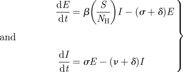4.8

where σ is the rate at which exposed individuals transition to becoming infectious.

The mean basic reproduction number for this class of models is given by [2]

4.9

This is because the rate at which an infected individual infects susceptible hosts is given by β, but only a fraction of them, (σ/(σ + δ)), will become infectious. The remaining fraction will die prior to becoming infectious. The variance in the basic reproduction number is given by

4.10

because the rate of infection loss is again constant, leading to an exponential distribution for the duration of time individuals remain infectious.

The two remaining quantities that require identification are τ and N. From equations (4.8), we might naively expect that the average amount of time it takes an individual to transmit the disease is

which is equivalent to

at endemic equilibrium. Although this is the case for δ ≪ σ, when this assumption is not met, 1/σ overestimates the average amount of time an individual who becomes infectious spends in the exposed class. To accurately calculate this time, we define 1/σ_adj as the average duration of time an individual spends in the exposed class, provided that he will transition to the infectious class. This mortality-adjusted expected time is given by [23]:

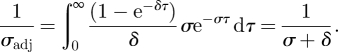4.11

The generation time τ is therefore

Finally, the relevant population size N is appropriately defined as the sum of the number of exposed individuals who will become infectious and the number of infectious individuals:

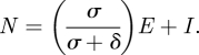4.12

This is because, over a single generation, viral lineages are transmitted by individuals who are either already infectious at the beginning of the generation or by individuals who are exposed at the beginning of the generation, but who will become infectious during the viral generation, as defined above. With these quantities, the rate of coalescence for SEIS/SEIR/SEIRS models becomes

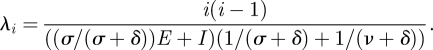4.13

Figure 1c shows a genealogy that has been simulated using equation (4.13). A lineages-through-time plot for this genealogy is shown in figure 1e. This plot indicates that lineages coalesce more slowly when an exposed period is present than when absent. Equation (4.13) indicates that this is because exposed individuals increase the effective population size and because the generation time is longer than the period of infectiousness.

We again used forward simulations to check the accuracy of our analytical results. As before, figure 4 plots the proportion of sample sets that had a first coalescence by the time indicated on the x-axis against our analytical expectation, indicating that equation (4.13) is accurate. This figure also shows that that the rate of coalescence is significantly overestimated if N is incorrectly specified as only the number of infectious individuals, and that the rate of coalescence can be significantly underestimated if the generation time τ is not adjusted for mortality from the exposed class.

Figure 4.

A comparison between analytical results and SEIR model simulations. The CDF for the time to coalescence computed from equation (4.13) is shown in solid black, and the simulation results from 1000 sample sets in solid grey. The dotted black line shows the CDF for the time to coalescence computed from The dashed black line shows the CDF for the time to coalescence computed from Parameters for the analytical results are i = 25 lineages, ν = 1/10 d⁻¹, δ = 1/3 yr⁻¹, σ = 1/2 yr⁻¹, E = 32 000 and I = 434. Parameters for the model simulations were N_H = 25 100 thousand, E[R₀] = 5, ν = 1/10 d⁻¹, δ = 1/3 yr⁻¹ and σ = 1/2 yr⁻¹, yielding E = 32 000 and I = 434 at equilibrium.

The average number of pairwise nucleotide differences π for this class of models is given by

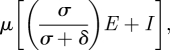which is higher than that for SIS/SIR/SIRS models. The rate of genetic drift is given by

which is lower than that for SIS/SIR/SIRS models.

4.4. SIS/SIR/SIRS models with variable distributions of the infectious period

SIS/SIR/SIRS models are frequently extended to allow for variable distributions for the amount of time individuals remain infectious. This is commonly done by using the method of stages [24]: simulating n > 1 compartments of infected individuals, with individuals moving from one compartment to the next compartment at a constant rate νn [1]:

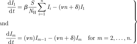4.14

Under this formulation, the average amount of time individuals remain infectious is 1/ν, provided that the mortality rate is negligible compared with the rate at which individuals transition between infected classes, δ ≪ νn. As n → ∞, all individuals remain infectious for 1/ν units of time. As n → 1, the duration of time individuals remain infectious becomes exponentially distributed, with the classic class of SIS/SIR/SIRS models recovered when n = 1.

To derive the rate of coalescence for this class of epidemiological models, we again need the relevant population size N, E[R₀], var(R₀) and τ. We derive these quantities here under the assumption that δ ≪ νn in order to highlight the parts of this class of models that makes them unique. A similar approach to the one described in the previous class of models, however, can be used to mortality-adjust transition rates if this assumption is violated. In the equations that follow, we therefore use the notation ‘≈’ rather than ‘=’ to remind the reader that these quantities are approximations.

Instead of deriving N, E[R₀] and var(R₀) independently, it is easier to derive N_e by writing 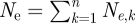, where N_e,k is the effective population size of individuals in infectious compartment k. The average reproduction number of individuals in compartment k is given by E[R_0,k] ≈ β/(νn), and the variance given by var(R_0,k) ≈ (β/(νn))² because the average duration of time individuals remain in compartment k is exponentially distributed with mean 1/(νn). Substituting into equations (3.4) and (2.6) yields N_e,k = I_k/2, such that the total effective population size becomes

Finally, we can turn to the generation time τ. At endemic equilibrium, the average amount of time it takes for individuals in the first infectious compartment to transmit is given by 1/(νn). The average amount of time, since infection, it takes for individuals in the second infectious compartment to transmit is given by 2/(νn). This is because it takes on average 1/(νn) amount of time for an individual in this second class to pass through the first class, and another 1/(νn) units of time for the individual to transmit while in this second class. Analogously, the average amount of time for an individual in the kth infectious class to transmit is given by k/(νn). With our assumption of δ ≪ νn, the number of individuals in each infectious class is the same, so that we can write the overall average time to the next transmission as

4.15

Putting these quantities together yields a rate of coalescence of

4.16

where 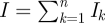. When the number of infectious compartments n is 1, this reduces to the family of models considered in our first application, and indeed the rate of coalescence becomes equation (4.2), once the mortality rate δ has been assumed negligible. As n approaches infinity, the average time to infection is cut in half, and the rate of coalescence is therefore twice as fast. Figure 1d shows a genealogy that has been simulated using equation (4.16), with n = 10 infectious classes, and figure 1e the corresponding lineages-through-time plot. A comparison between the number of lineages through time under this model versus the SIS/SIR/SIRS model indicates that lineages coalesce more rapidly when the duration of infection is less variable among infected individuals, as expected by the higher rate of coalescence brought about by the shortening of the generation time.

To check the accuracy of our analytical results, we simulated three models of this class, with n = 1, 3 and 10 infectious compartments, keeping the average infectious period 1/ν constant across the simulations. Figure 5 plots the proportion of sample sets from each of these three simulations that had a first coalescence by the time indicated on the x-axis. Comparisons against the CDFs calculated using the coalescent rate provided in equation (4.16) indicates that our analytical results are accurate.

Figure 5.

A comparison between analytical results and simulations of an SIR model with variable distributions of the infectious period. The CDFs for the time to coalescence computed from equation (4.16) are shown with solid lines, with n = 1 infectious compartment in blue, n = 3 infectious compartments in black and n = 10 infectious compartments in red. The simulation results from 1000 sample sets are shown with dashed lines, with colours corresponding to the number of infectious compartments. Parameters for the analytical results are i = 25 lineages, ν = 1/10 d⁻¹, I = 7819 and n = 1, 3 or 10. Parameters for the model simulations were N_H = 25 million, E[R₀] = 5, ν = 1/10 d⁻¹, δ = 1/70 yr⁻¹, and n = 1, 3, or 10. In all three cases, I = 7819 at equilibrium.

As before, the average number of pairwise nucleotide differences π and rates of genetic drift can be computed using the effective population size and the generation time. The mean level of genetic diversity is, as before, given by 2μI, where μ is the per generation mutation rate. Although this level of genetic diversity initially appears to be the same as the one for SIS/SIR/SIRS models, if instead we consider that the mutation rate is more likely to be constant in terms of calendar time than generation time, we should instead write π as

with μ_c as the mutation rate per unit of calendar time. In this case, because of the shorter generation time when n > 1, the amount of viral diversity is expected to be smaller than for SIS/SIR/SIRS models. The rate of genetic drift for these models is given by

which is higher than that for SIS/SIR/SIRS models.

5. Discussion

Here, we have presented a general approach to derive rates of coalescence for a wide range of epidemiological models at their endemic equilibrium and have applied this approach to four common families of epidemiological models. The different rates of coalescence between these models indicate that the structures of epidemiological models leave imprints on the shapes of viral gene genealogies. While it is well known that population size dynamics affect the shapes of viral genealogies [25], the observation that viral genealogies are also affected by factors such as the extent of disease supershedding, the presence of exposed periods and the distribution of infectious periods is novel.

The derivation of the rates of coalescence for the four families of epidemiological models we considered is not meant to be exhaustive. Many of the epidemiological models used today combine several components of the models we considered. For example, a disease may have a latent period prior to an infected person becoming infectious and also be highly variable in transmissibility among individuals. This combines the model of the third application with the model of the second application. From the general approach we outlined for deriving rates of coalescence, these more complex epidemiological models can nevertheless be easily considered by correctly specifying the relevant population size N and the relevant generation τ, and by deriving the mean and variance of individuals' basic reproduction number distribution.

The ability to derive coalescent rates and effective population sizes specific to an epidemiological model is useful for several reasons. First, sequence data are now routinely used to reconstruct the demographic histories of viral populations, commonly visualized in the Bayesian skyline plot [6]. When sequences are serially sampled, these histories are given as the product of the effective population size and the generation time. Knowledge of how N_e and τ are affected by epidemiological factors such as exposed periods, the distribution of infectious periods and the extent of supershedding, will therefore help us be able to better interpret the magnitude of N_eτ and may help us understand why, for example, a disease with low prevalence and a short duration of infection may nevertheless have higher θ values than a persistent disease with high prevalence. (As shown here, a lower variability in transmission rates or a long exposed period in the former case may result in an overall higher N_eτ, despite a lower prevalence level and a shorter duration of infection.)

Second, statistical inference methods that seek to fit complex epidemiological models to viral genetic data will require model-specific coalescent rate expressions. This is because these rates provide the quantitative link between the structures and parameters of epidemiological models and the machinery of population genetics used to evaluate the probability of a genealogy given these models. Several statistical approaches already exist, but they have all been based on the simplest of epidemiological models (e.g. SI, SIS or SIR models) [11–13]; the consideration of more complex epidemiological models, such as the ones presented in applications 4.1 through 4.4, will therefore require an a priori appropriate specification of coalescent rates. Our general approach thereby facilitates the extension of existing methods to consider more realistic epidemiological processes.

We caution the reader, however, in directly applying the general approach outlined here to derive model-specific coalescent rates for statistical inference methods. This is for several reasons. First, we have generally written the generation time τ in terms of the average duration of infection, rather than in terms of the average time it takes for an infected individual to transmit the disease (which has been termed the generation interval [26]). At endemic equilibrium, these two quantities are equal. However, during the rise of an epidemic, the generation interval is shorter than the average duration of infection [26]. Similarly, during the fall of an epidemic, the generation interval is longer than the average duration of infection. Care therefore needs to be taken to appropriately define τ when dynamics are not at equilibrium.

Second, the formulation presented here is only valid if the transmission term is linear in the number of infecteds (i.e. if the transmission term is of the form βS^γI^α, where α = 1; E. Volz 2011, personal communication). This can be seen by returning to the rate of coalescence derived in Volz et al. [12], shown in equation (4.3), which does not assume equilibrium conditions. When the transmission term is linear in the number of infected individuals, the I in the numerator and denominator cancel and the resulting rate of coalescence can be seen as only depending inversely on disease prevalence I (and directly on the number of susceptible hosts). However, when α ≠ 1, the I's do not simply cancel, and the rate of coalescence can therefore never be described in terms of the N_eτ formalism. However, most epidemiological models that are commonly used are linear in I, so we do not consider this a major limitation.

Finally, the general approach detailed here is limited in that it cannot be accurately applied to non-equilibrium situations when the population of infected individuals is structured in some way. For example, SEIR models are structured: infected individuals are classified as exposed (E) or infectious (I). Models with variable distributions of the infectious period are similarly structured, because distinct infectious classes exist (I₁, I₂, … , I_n). The approach outlined here is not suitable for these situations because the rate of coalescence should depend on the number of individuals in each compartment, not just their sum. For example, if all individuals infected in an SEIR model belonged to the I class and none to the E class at time t, then the instantaneous rate of coalescence at time t should be zero. This is because lineage coalescence can only occur when an infected individual has just infected a susceptible individual; backwards in time, this means that for there to be a positive rate of coalescence, both exposed and infected individuals need to be present in the population. The number of individuals in each class of infected individuals therefore matters, not only their sum.

Despite these limitations, some of the rates derived here can be directly integrated into current statistical inference methods (e.g. [13]). For example, the rate of coalescence derived for SIS/SIR/SIRS models, given by equation (4.2), can be applied to non-equilibrium dynamics as long as τ is redefined as 1/[β(S/N_H)]. This is similarly so for the rate of coalescence derived for SIS/SIR/SIRS models with supershedding, given by equation (4.7). Furthermore, the work presented here can also be used to check the accuracy of coalescent rate expressions that have been more generally derived for structured populations with non-equilibrium dynamics: when considered at equilibrium, the rate expressions should be identical.

The work presented here therefore highlights the role that epidemiological model structures can play in shaping viral genealogies. Most importantly, our general approach for deriving rates of coalescence for models at endemic equilibrium shows how characteristics of the infection process alter effective population sizes and generation times. As such, it provides an intuitive framework for better understanding observed patterns of viral diversity. However, as elaborated on above, our approach has only limited applicability to non-equilibrium systems. It therefore points towards the need for an even more general approach that would enable a more effective use of viral genetic data for gaining insight into the factors driving infectious disease dynamics.

References

- 1.Lloyd A. L. 2001. Destabilization of epidemic models with the inclusion of realistic distributions of infectious periods. Proc. R. Soc. Lond. B 268, 985–993 10.1098/rspb.2001.1599 (doi:10.1098/rspb.2001.1599) [DOI] [PMC free article] [PubMed] [Google Scholar]
- 2.Keeling M. J., Rohani P. 2008. Modeling infectious diseases in humans and animals. Princeton, NJ: Princeton University Press [Google Scholar]
- 3.Lloyd-Smith J. O., Schreiber S. J., Kopp P. E., Getz W. M. 2005. Superspreading and the effect of individual variation on disease emergence. Nature 438, 355–359 10.1038/nature04153 (doi:10.1038/nature04153) [DOI] [PMC free article] [PubMed] [Google Scholar]
- 4.Drummond A. J., et al. 2002. Estimating mutation parameters, population history and genealogy simultaneously from temporally spaced sequence data. Genetics 161, 1307–1320 [DOI] [PMC free article] [PubMed] [Google Scholar]
- 5.Rodrigo A. G. 2009. The coalescent: population genetic inference using genealogies. In The phylogenetic handbook: a practical approach to phylogenetic analysis and hypothesis testing (eds Lemey P., Salemi M., Vandamme A. M.). Cambridge, UK: Cambridge University Press [Google Scholar]
- 6.Drummond A. J., Rambaut A., Shapiro B., Pybus O. G. 2005. Bayesian coalescent inference of past population dynamics from molecular sequences. Mol. Biol. Evol. 22, 1185–1192 10.1093/molbev/msi103 (doi:10.1093/molbev/msi103) [DOI] [PubMed] [Google Scholar]
- 7.Drummond A. J., Rambaut A. 2007. BEAST: Bayesian evolutionary analysis by sampling trees. BMC Evol. Biol. 7, 214. 10.1186/1471-2148-7-214 (doi:10.1186/1471-2148-7-214) [DOI] [PMC free article] [PubMed] [Google Scholar]
- 8.Griffiths P. D., Tavaré S. 1994. Sampling theory for neutral alleles in a varying environment. Phil. Trans. R. Soc. Lond. B 344, 403–410 10.1098/rstb.1994.0079 (doi:10.1098/rstb.1994.0079) [DOI] [PubMed] [Google Scholar]
- 9.Rodrigo A. G., Shpaer E. G., Delwart E. L., Iversen A. K. N., Gallo M. V., Brojatsch J., Hirsch M. S., Walker B. D., Mullins J. I. 1999. Coalescent estimates of HIV-1 generation time in vivo. Proc. Natl Acad. Sci. USA 96, 2187–2191 10.1073/pnas.96.5.2187 (doi:10.1073/pnas.96.5.2187) [DOI] [PMC free article] [PubMed] [Google Scholar]
- 10.Fraser C., et al. 2009. Pandemic potential of a strain of influenza A (H1N1): early findings. Science 324, 1557–1561 10.1126/science.1176062 (doi:10.1126/science.1176062) [DOI] [PMC free article] [PubMed] [Google Scholar]
- 11.Pybus O. G., Charleston M. A., Gupta S., Rambaut A., Holmes E. C., Harvey P. H. 2001. The epidemic behavior of the hepatitis C virus. Science 292, 2323–2325 10.1126/science.1058321 (doi:10.1126/science.1058321) [DOI] [PubMed] [Google Scholar]
- 12.Volz E. M., Kosakovsky Pond S. L., Ward M. J., Leigh Brown A. J., Frost S. D. W. 2009. Phylodynamics of infectious disease epidemics. Genetics 183, 1421–1430 10.1534/genetics.109.106021 (doi:10.1534/genetics.109.106021) [DOI] [PMC free article] [PubMed] [Google Scholar]
- 13.Rasmussen D. A., Ratmann O., Koelle K. In press Inference for nonlinear epidemiological models using genealogies and time series. PLoS Comput. Biol. 7, e1002136. 10.1371/journal.pcbi.1002136 (doi:10.1371/journal.pcbi.1002136) [DOI] [PMC free article] [PubMed] [Google Scholar]
- 14.Frost S. D. W., Volz E. M. 2010. Viral phylodynamics and the search for an ‘effective number of infections’. Phil. Trans. R. Soc. Lond. B 365, 1879–1890 10.1098/rstb.2010.0060 (doi:10.1098/rstb.2010.0060) [DOI] [PMC free article] [PubMed] [Google Scholar]
- 15.Rohani P., Keeling M. J., Grenfell B. T. 2002. The interplay between determinism and stochasticity in childhood diseases. Am. Nat. 159, 469–481 10.1086/339467 (doi:10.1086/339467) [DOI] [PubMed] [Google Scholar]
- 16.Coulson T., Rohani P., Pascual M. 2004. Skeletons, noise and population growth: the end of an old debate? Trends Ecol. Evol. 19, 359–364 10.1016/j.tree.2004.05.008 (doi:10.1016/j.tree.2004.05.008) [DOI] [PubMed] [Google Scholar]
- 17.Kingman J. F. C. 1982. The coalescent. Stoch. Process. Appl. 13, 235–248. [Google Scholar]
- 18.Wakeley J. 2008. Coalescent theory: an introduction USA: Roberts & Company [Google Scholar]
- 19.Nordberg M. 2001. Coalescent theory. In Handbook of statistical genetics (eds Balding D., Bishop M., Canning C.), pp. 179–212 New York, NY: Wiley & Sons [Google Scholar]
- 20.Sjödin P., Kaj I., Krone S., Lascoux M., Nordborg M. 2005. On the meaning and existence of an effective population size. Genetics 169, 1061–1070 10.1534/genetics.104.026799 (doi:10.1534/genetics.104.026799) [DOI] [PMC free article] [PubMed] [Google Scholar]
- 21.Gillespie D. T. 1976. A general method for numerically simulating the stochastic time evolution of coupled chemical reactions. J. Comput. Phys. 22, 403–434 10.1016/0021-9991(76)90041-3 (doi:10.1016/0021-9991(76)90041-3) [DOI] [Google Scholar]
- 22.Goodman L. A. 1960. On the exact variance of products. J. Am. Stat. Assoc. 55, 708–713 10.2307/2281592 (doi:10.2307/2281592) [DOI] [Google Scholar]
- 23.Blythe S. P., Anderson R. M. 1988. Distributed incubation and infectious periods in models of the transmission dynamics of the human immunodeficiency virus (HIV). IMA J. Math. Appl. Med. Biol. 5, 1–19 10.1093/imammb/5.1.1 (doi:10.1093/imammb/5.1.1) [DOI] [PubMed] [Google Scholar]
- 24.Anderson D., Watson R. 1980. On the spread of a disease with gamma distributed latent and infectious periods. Biometrika 67, 191–198 10.1093/biomet/67.1.191 (doi:10.1093/biomet/67.1.191) [DOI] [Google Scholar]
- 25.Grenfell B. T., Pybus O. G., Gog J. R., Wood J. L. N., Daly J. M., Mumford J. A., Holmes E. C. 2004. Unifying the epidemiological and evolutionary dynamics of pathogens. Science 303, 327–332 10.1126/science.1090727 (doi:10.1126/science.1090727) [DOI] [PubMed] [Google Scholar]
- 26.Kenah E., Lipsitch M., Robins J. M. 2008. Generation interval contraction and epidemic data analysis. Math. Biosci. 213, 71–79 10.1016/j.mbs.2008.02.007 (doi:10.1016/j.mbs.2008.02.007) [DOI] [PMC free article] [PubMed] [Google Scholar]