

Abstract
Motivation: Protein–protein interactions (PPIs) are a promising, but challenging target for pharmaceutical intervention. One approach for addressing these difficult targets is the rational design of small-molecule inhibitors that mimic the chemical and physical properties of small clusters of key residues at the protein–protein interface. The identification of appropriate clusters of interface residues provides starting points for inhibitor design and supports an overall assessment of the susceptibility of PPIs to small-molecule inhibition.
Results: We extract Small-Molecule Inhibitor Starting Points (SMISPs) from protein-ligand and protein–protein complexes in the Protein Data Bank (PDB). These SMISPs are used to train two distinct classifiers, a support vector machine and an easy to interpret exhaustive rule classifier. Both classifiers achieve better than 70% leave-one-complex-out cross-validation accuracy and correctly predict SMISPs of known PPI inhibitors not in the training set. A PDB-wide analysis suggests that nearly half of all PPIs may be susceptible to small-molecule inhibition.
Availability: http://pocketquery.csb.pitt.edu.
Contact: dkoes@pitt.edu
Supplementary information: Supplementary data are available at Bioinformatics online.
1 INTRODUCTION
Protein–protein interactions (PPIs) play a key role in nearly every biological function and are a promising new class of biological targets for therapeutic intervention (Dömling, 2008; Wells and McClendon, 2007). PPIs present a number of unique challenges compared to targets that have historically dominated pharmaceutical efforts, such as enzymes, G-protein-coupled receptors, and ion-channels (Paolini et al., 2006). Unlike these targets, which have evolved to bind small molecules, PPIs have no convenient natural substrate to serve as a starting point for small-molecule design. However, alanine scanning mutagenesis reveals that most of the energy of a PPI is contributed by just a few ‘hot spot’ residues (Clackson and Wells, 1995; Moreira et al., 2007; Rajamani et al., 2004). A small cluster of co-located interface residues that includes at least one hot spot provides a starting point for the rational design of small molecule inhibitors (Meireles et al., 2010). Indeed, the chemical mimicry of small clusters of key residues, typically deeply buried ‘anchor’ residues (Rajamani et al., 2004), has produced inhibitors for several PPI targets (Christ et al., 2010; Liu et al., 2007; Popowicz et al., 2011).
The importance of hot spot residues and the difficulty in performing alanine scanning mutagenesis has led to the development of several computational methods for predicting hot spots. Energy-based methods (Camacho and Zhang, 2005; Kortemme et al., 2004) attempt to directly compute the energetic contributions of residues. Solvent accessible surface area (SASA) (Meireles et al., 2010; Rajamani et al., 2004) and sequence conservation (Bromberg and Rost, 2008; Keskin et al., 2005; Lichtarge et al., 1996; Ofran and Rost, 2007) have also been used to predict hot spots. However, the most successful computational methods use some combination of these and other features (Cho et al., 2009; Darnell et al., 2007; Guney et al., 2008; Lise et al., 2009; Tuncbag et al., 2009; Zhu and Mitchell, 2011) and achieve accuracies of 60–80%. Often a consensus scoring mechanism is derived using machine learning techniques such as decision trees (Darnell et al., 2007) or support vector machines (Cho et al., 2009; Lise et al., 2009), although ad hoc consensus schemes are effective as well (Guney et al., 2008; Tuncbag et al., 2009).
In order to enhance specificity and affinity, additional interactions beyond those present in a single individual hot spot residue are needed. Nearby residues that do not meet the criteria of a hot spot may also play an important, if not essential, role in the interaction. Additionally, these residues may describe extra pockets or energetics essential for small molecule binding or specificity. Although identifying a minimum set of stereochemical properties consistent with a small-molecule binding site is challenging (Hajduk et al., 2005; Pérot et al., 2010), the increasing number of ligand-protein and protein–protein structures in the Protein Data Bank (PDB) provides a foundation to explore this important problem with respect to PPIs. In fact, a systematic analysis of such structures reveals that residues that participate in both ligand and protein binding have distinctly different characteristics from other interface residues (Davis and Sali, 2010). This important insight suggests that it may be possible to automatically identify those interface residues that are most susceptible to small-molecule intervention.
In this work we describe a novel structural bioinformatics approach that identifies and ranks those clusters of interface residues in a PPI that are most suitable as starting points for rational small-molecule design. We refer to these clusters as Small-Molecule Inhibitor Starting Points (SMISPs). A SMISP is larger than a hot spot, but substantially smaller than the entire collection of interface residues. A SMISP cluster may include both those residues critical to the protein–protein interaction and those with features important for binding specificity, all within a volume accessible to a small molecule.
SMISPs are complementary to approaches that identify binding sites through an analysis of the receptor surface (Henrich et al., 2010), either through shape descriptors (Weisel et al., 2007) or chemical probes (Brenke et al., 2009; Fuller et al., 2009). However, a SMISP, as a collection of interface residues, not only defines a binding site, it also defines a binding mode selected by evolution that provides an initial target for rational small-molecule design. More general binding site identification techniques can then provide insight on how to extend this natural site or explore the flexibility of the site.
Previous work has identified clusters of interface residues from helical interfaces as small-molecule starting points (Jochim and Arora, 2010). A manually specified energy criteria based off of computational alanine scanning (Kortemme et al., 2004) was used to identify co-located hot spots on a helix that provided a significant portion of the free energy of the helical interaction. This method is only partially successful at identifying SMISPs corresponding to known PPI inhibitors. In addition to being limited to helical interfaces, we find the energy criteria used to be less informative in characterizing SMISPs than SASA and alternative energy calculations. Our approach, which uses a consensus score, is more successful at recovering SMISPs of known inhibitors.
In a departure from analyses that calibrate to free energies from alanine scanning experiments, we identify SMISPs directly from protein–protein and protein-ligand structures. From this structural analysis we develop a consensus score based on physical and evolutionary descriptors for predicting and ranking SMISPs. We develop a methodology for learning two distinct classifiers: an exhaustive rule classifier for filtering SMISPs using an easy to interpret rule and a support vector machine (SVM) classifier for ranking SMISPs. Our approach allows us to examine the importance and role of various factors, such as SASA and free energy estimates, in defining SMISPs. We demonstrate the ability of our predicted SMISPs to identify known PPI inhibition sites. Finally, a PDB-wide analysis predicts the existence of suitable small-molecule inhibitor starting points in 48% of protein–protein interactions.
2 METHODS
We use machine learning techniques to learn both filtering and scoring criteria for identifying SMISPs. Similar approaches have successfully been used to identify hot spot residues and interface residues (Cho et al., 2009; Darnell et al., 2007; Lise et al., 2009). For these problems, experimental data, in the form of alanine scanning experiments and PPI crystal structures, is readily available. In order to generate a similar benchmark set of SMISPs, we mine the structural data in the PDB by identifying PPI interface residues that overlap with known small-molecule binding sites. We annotate all clusters of interface residues with aggregate indicators of energy, SASA, and sequence conservation. This benchmark set is then used to train both an exhaustive rule classifier, which generates an easy to interpret filter, and an SVM classifier, which produces a numerical score. The complete workflow of our method is shown in Figure 1.
Fig. 1.

The complete workflow of our method. A benchmark of small molecule inhibitor starting points (SMISPs) is extracted from the structural information of protein–protein and protein-ligand complexes in the PDB. A training set is generated from this benchmark and used to train both a rule-based and SVM classifer which then back-annotate an entire non-redundant subset of PPI complexes from the PDB.
To support a PDB-wide analysis, we first generate a non-redundant subset of PPI complexes. We use the search feature of the PDB to retrieve all protein-only structures with at least two chains in the biological assembly with a resolution of less than 4.0 that have less than 95% sequence similarity resulting in 13,413 structures (downloaded 6/25/2011). After removing misclassified, non-interacting, or otherwise unanalyzable assemblies, 12,456 complexes remain to form our non-redundant set of PPI structures.
2.1 Benchmark set
Protein–protein interactions remain a challenging and relatively untargeted area of pharmaceutical intervention resulting in a scarcity of proven small-molecule starting points. However, an analysis of the structures deposited in the PDB reveals that for many PPIs there exists a structure where at least one chain of the PPI is complexed with a small molecule that binds at the PPI interface site. A sufficiently high-affinity small-molecule targeting such a site will, at the very least, perturb the interaction. Consequently, we utilize such ligand-bound structures to identify benchmark SMISPs in the original PPI. A benchmark SMISP is the collection of all interface residues from a PPI structure that overlap a high-affinity ligand from a protein-ligand structure aligned to the PPI structure. A benchmark SMISP at least partially delineates the binding site of the ligand, thus providing a validated starting point for the design of a small-molecule inhibitor.
For each chain of each complex in our non-redundant set, we identify all structures in the PDB that have 95% or greater sequence similarity to this receptor chain and that are bound to a standalone ligand (i.e., not a modified residue). We consider only ligands with a molecular weight greater than 150 Da to eliminate non-specific interactions such as ions and crystallographic buffers. We then align the ligand-bound structure to the original PPI complex. The collection of at least two PPI interface residues that contain atoms that overlap the atoms of the ligand in the ligand-bound structure in this aligned assembly is marked as a SMISP. Atom centers must be less than 2.5Å apart for atoms of the ligand and a residue to be considered overlapping (i.e., less than the distance of a hydrogen bond).
In some cases the ligand-bound structure is not a single chain protein, but a protein–protein complex that is homologous to the original PPI complex. In this case we impose an additional constraint that the backbone in the region of the SMISP residues be substantially distorted from the original PPI backbone (the root mean square deviation should be more than 1Å). These ligands do not prevent the formation of the protein–protein complex, since they bind to the fully formed complex, but we include them in the benchmark set since a significant perturbation of the interface structure will likely affect the function of the PPI.
We further refine our collection of SMISPs derived from structure by incorporating binding affinity data from the PDBbind (Wang et al., 2005), BindingDB (Liu et al., 2006), and Binding MOAD (Hu et al., 2005) databases. We restrict our benchmark SMISPs to only those where the ligand bound structure (or a homologue with at least 95% sequence identity) has an affinity of 100 μM or better to exclude spurious or low-affinity ligand-protein interactions. The resulting collection of SMISPs includes 135 distinct SMISPs derived from 267 ligands targeting 51 PPI complexes. There are nearly twice as many ligands as SMISPs since in most cases ligands targeting the same protein define identical or nearly identical SMISPs. Two SMISPs from this set, both derived from known PPI inhibitors, are shown in Figure 2. The SMISPs sterically delineate part of the binding site of the ligand in the unliganded complex. SMISPs cannot identify binding pockets that require a conformational change of the receptor complex, such as in Figure 2b where the ligand partially binds to a groove not present in the PPI structure. Our complete set of benchmark SMISPs is available in the Supplementary Data.
Fig. 2.
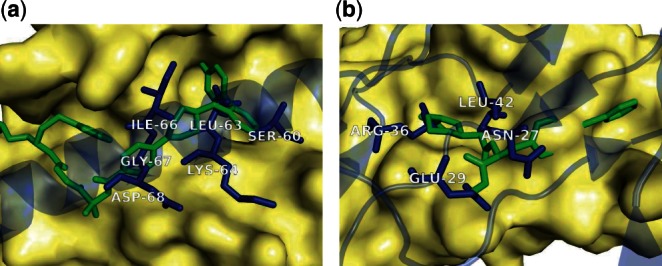
Example training SMISPs. The PPI is represented by a receptor protein (yellow surface) and a ligand protein (transparent blue). A small-molecule inhibitor (green) is posed by aligning the corresponding receptors. Training SMISPs (blue), clusters of interface residues that overlap the ligand, identify the binding pocket, but are not required to reproduce the exact interactions of the ligand. (a) Bcl-xL in complex with the BaxBH3 domain (PDB: 3PL7) is shown with the sub-nM inhibitor ABT-737 (PDB: 2YXJ). The LEU-63 residue of the SMISP fills a deep hydrophobic pocket that is also filled by the inhibitor, while ILE-68 fills a hydrophobic pocket that closes around the inhibitor in the ligand bound structure. The backbones of the remaining residues serve to further delineate the inhibitor binding site. (b) The interleukin-2 cytokine receptor complex (PDB: 2B5I) shown with an 8μM inhibitor (PDB: 1M48). The positively charged guanidinium group of ARG-36 overlays a guanidinium on the inhibitor while LEU-42 fills a hydrophobic pocket that closes around the inhibitor in the ligand-bound structure. GLU-29 and ASN-27 delineate a polar region of the receptor that is only partially targeted by the inhibitor as this region has a significantly different conformation in the ligand-bound structure.
2.2 Cluster features
We decompose PPI structures into clusters of multiple interface residues where each cluster will be evaluated for its potential to be a SMISP. An interface residue is defined as a residue where the change in SASA upon complexation is more than 0.05Å2. All SASA calculations are performed using naccess (http://www.bioinf.manchester.ac.uk/naccess/). To limit clusters to a volume accessible by small molecules, we consider only clusters where the centers of mass of any two residues in the cluster are less than 12Å apart. This distance is roughly equal to two turns of an α-helix and encompasses a volume larger than the 500Å3 usually observed in protein-ligand interactions (An et al., 2005).
For every cluster of interface residues, we generate a collection of aggregate features for use in SMISP classification. For each residue in the cluster we compute two energy scores, ΔGFC and ΔΔGR, the absolute ($ΔSASA) and the relative ($ΔSASA%) change in solvent accessible surface area, and two measures of sequence conservation, an evolutionary rate (Rate) and a conservation score (Cons). These features are aggregated into the minimum, maximum, average, and total value for each cluster. For all calculations, we use the first biological assembly deposited in the PDB and preprocess the structure with CHARMM version 31b1 (Brooks et al., 1983). CHARMM is used to add missing atoms, including hydrogens, and to quickly minimize the resulting structure to optimize hydrogen bonding.
ΔGFC FastContact (Camacho and Zhang, 2005) is used to compute a per-residue estimate of the free energy (kcal/mol) of complexation. It includes both electrostatic (ΔGFCelec) and desolvation ( ΔGFCdsolv) effects within an atomistic pair-wise potential. More negative values indicate energetically favorable residues.
ΔΔGR We use version 3.2.1 of the Rosetta software (Kortemme et al., 2004) to perform computational alanine scanning. The AlaScan filter is used with the ΔΔG optimized scoring function, an interface distance cutoff of 10Å, five repeats, and an initial local refinement docking. This value represents the change in free energy of the alanine mutation, so a larger, more positive value indicates that the alanine mutation destabilizes the complex and the original residue is a hot spot.
ΔSASA The change in absolute SASA of a residue is calculated by subtracting the SASA of the residue in the PPI complex from the SASA of the residue when all other protein chains have been removed from the PPI structure. That is, the bound conformation of the chain of the residue is used to compute the un-complexed SASA.
ΔSASA% The change in the relative SASA of a residue. Expressed as a percentage of accessible surface area.
Rate A multiple sequence alignment (MSA) of related sequences is obtained by using BLAST (Altschul et al., 1990) to retrieve the 20 most similar sequences from the UniRef90 database (Wu et al., 2006) and aligning the results with ClustalW version 2.0 (Larkin et al., 2007). An evolutionary rate for each residue is computed using Rate4Site version 2.01 (Mayrose et al., 2004). Rate4Site uses an empirical Bayesian method to compute an evolutionary rate from a phylogenetic tree it constructs from the MSA. A higher score indicates a higher rate and lower degree of conservation. If there are no similar sequences in UniRef90 (for example, when searching for a short peptide), then no value is generated.
Cons An MSA is generated as above and a conservation score is computed using Scorecons (Valdar, 2002) with the default parameters. The score is a function of the sum-of-pairs pairwise match within the MSA, a substitution matrix, and a sequence weighted normalization. A higher score indicates a higher degree of conservation.
2.3 Training
We utilize two classification methods a support vector machine (SVM) classifier and an exhaustive rule classifier. We construct a balanced training set from our benchmark SMISPs, and we use leave-one-complex-out cross-validation to parameterize the classifiers and assess their accuracy.
Training set We construct a training set from the benchmark set that is evenly distributed among the PPI structures: for each PPI we generate 100 positive examples and 100 negative examples.
Positive examples are selected by combining the SMISP benchmark set with the 12Å clusters. Only the largest clusters that are fully contained within a benchmark SMISP are selected. In most cases, this results in positive examples that are identical to the benchmark SMISPs, but five training set PPIs have large benchmark SMISPs that are decomposed into all possible maximal subsets of residues that fit within a 12Å distance cutoff.
Negative examples are generated by selecting clusters of interface residues from the same chain(s) as the benchmark SMISPs that are equal in size to the SMISPs selected as positive examples and in no way overlap any benchmark SMISPs of the PPI.
Since the number of negative examples is typically much larger than the number of positive examples and SVMs perform poorly on imbalanced training data, we re-sample the data to create a balanced training set (Batuwita and Palade, 2010). For both positive and negative examples, random selection with replacement is performed. A sample size of 100 was found to produce stable results across multiple trials of random sampling.
Missing values, which are present for the sequence conservation scores when no similar sequences are found, are replaced by average values. Twelve PPIs in the benchmark set contain no negative examples because the ligand protein of the PPI is a short peptide where all, or nearly all, of the interface residues make up a SMISP. Since the entire peptide defines a SMISP, these 12 PPIs are trivial to identify as SMISPs and are excluded from the training set. There are a total of 7800 training examples from 39 PPI complexes. The composition of the training set is further described in the Supplementary Data.
Leave-one-complex-out validation is performed by removing all training examples of a PPI complex from the training set and then using these examples as a test set resulting in 39 unique train-test datasets. The cross-validation accuracy (correct predictions divided by total predictions) is computed by taking the average across these datasets.
Validation set In order to qualitatively characterize the performance of our classifiers, we construct a validation set of 11 PPI complexes with known inhibitors where both the protein–protein and protein-ligand structures are available. These complexes were identified from recent publications (Stewart et al., 2010; Wells and McClendon, 2007) and PPI databases (Bourgeas et al., 2010; Higueruelo et al., 2009) and are shown in Table 1. These complexes did not appear in the training set because the inhibitor was not present in the binding affinity databases or a sufficiently homologous complex was not available in the non-redundant subset. We do not consider three PPIs (PDBs: 1DT7, 1TNR, 2NOD) with known inhibitors and structure where the inhibitor binding site does not overlap the PPI interface. These inhibitors are presumed to function allosterically and are beyond the scope of our SMISP classification. The only overlap between this validation set and the training set is with the Bcl-xL/BaxBH3 complex of Figure 2b. The validation set includes a Bcl-xL/Beclin 1 complex and a Bcl-2/BaxBH3 complex.
Table 1.
Validation set of PPIs with known inhibitors
| Description | PPI PDB | Ch | Lig. PDB | #SMISPs | #Clust |
|---|---|---|---|---|---|
| p53/MDM2 | 1YCR | B | 3LBK | 100 | 311 |
| p53/MDM4 | 3DAB | B | 3LBJ | 45 | 79 |
| XIAP/Caspase-9 | 1NW9 | B | 3CLX | 30 | 537 |
| XIAP/Smac | 1G73 | A | 2JK7 | 117 | 1793 |
| HIV gp41 | 1AIK | C | 2KP8 | 66 | 639 |
| Bcl-xL/Beclin 1 | 2P1L | B | 2O2N | 572 | 1503 |
| Bcl-2/BaxBH3 | 2XA0 | C | 2O22 | 762 | 1327 |
| HIV-1 Integrase/p75 | 2B4J | C | 3LPT | 36 | 123 |
| ZipA/FtsZ | 1F47 | A | 1Y2F | 40 | 263 |
| HPV E1/E2 | 1TUE | A | 1R6N | 56 | 312 |
| TNF- α | 1TNF | C | 2AZ5 | 80 | 2979 |
PPIs were identified from the literature (Bourgeas et al., 2010; Higueruelo et al., 2009; Stewart et al., 2010; Wells and McClendon, 2007) and only inhibitors with known structure that bind at the PPI interface are considered. The number of SMISPs predicted by our combined classifier is shown with the total number of clusters evaluated. As clusters are all possible collections of co-located interface residues, the number of clusters is combinatorially related to the number of interface residues.
SVM classifier We train our SVM classifier using the recommended procedure for libSVM (see Supplementary Data). The pairwise coupling method (Wu et al., 2004) is used to generate probability estimates for scoring potential SMISPs. The best cross-validation accuracy (74%) is obtained with a score threshold of 0.55. Higher score thresholds increase the specificity, but at the cost of substantially reduced recall. The average of the areas under the cross-validation receiver operating characteristic (ROC) curves is 0.82. Complete performance metrics for a variety of score thresholds are available in Supplemental Table S1 and the ROC curve is shown in Supplemental Figure S4.
Exhaustive rule classifier Previous work with hot spot prediction (Tuncbag et al., 2009) has shown that simple thresholding rules, e.g. ΔSASA > 60, can be as effective as more sophisticated classifiers. Such rules have the advantage of being easy to interpret and modify. However, they produce a strict binary classification and cannot be used to score and rank inputs.
Our rule classifier identifies rules that maximize the information gain. The information gain (IG) of a rule is the expected reduction in Shannon entropy if the result of applying the rule to the input dataset is known:
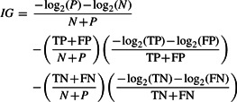 |
where N and P are the number of negative and positive examples and TP, FP, TN, and FN are the number of true positives, false positives, true negatives and false negatives after classification with the rule. An information gain of one is only possible if the rule perfectly classifies the dataset, and an information gain of zero implies the rule is no better than random.
We use an exhaustive rule classifier to generate the conjunctive rule of a given set of attributes that maximizes the information gain. The optimal set of thresholds is found through an exhaustive exploration that is accelerated using branch and bound techniques (Rijnbeek and Kors, 2010). The advantage of our exhaustive rule classifier is that the thresholds for different attributes are determined simultaneously and optimally, in contrast to methods, such as decision trees, that greedily select and set attributes and thresholds. The C/C++ source code of our implementation is available in the Supplementary Data.
We cross-validated our classifier using all possible one, two, and three attribute rules to identify the most accurate and informative attributes. The addition of a third attribute does not meaningfully improve the performance of the classifier: the most informative two attribute and three attribute rules both have a cross validation accuracy of 72%. Since the addition of a third attribute does not improve performance, we consider no more than two attributes per rule to avoid over-fitting the data.
3 RESULTS
We analyze the information theoretic properties of our cluster features to highlight the most useful features for classification. We show that we can recover known PPI inhibitor sites and assess the general accessibility of PPIs to small-molecule inhibitors.
3.1 Information gain analysis
A selection of cluster features are shown ranked by the information gain of the corresponding single-attribute rule in Table 2. The single most informative feature is the average ΔSASA. Average ΔSASA% and ΔGFC are also informative and have good classification accuracies. These average values, which represent the entire cluster, are more informative than extrema values of the same criteria (maximum surface area or minimum energy) that only represent the ‘hottest’ residue in the cluster. This underscores the value of our approach, which analyzes clusters as a unit, as opposed to an approach that simply identifies co-located hot spots.
Table 2.
Single attribute rules.
| Info. Gain | Rule | Accuracy (%) | ||
|---|---|---|---|---|
| 0.137 | Ave | ΔSASA | ≥44.6 | 68 ± 3.6 |
| 0.128 | Ave | ΔSASA% | ≥39.6 | 68 ± 3.7 |
| 0.103 | Ave | ΔGFC: | <−2.3 | 67 ± 3.9 |
| 0.081 | Ave | ΔGFCdsolv: | <−1.64 | 61 ± 3.4 |
| 0.070 | Max | ΔΔGR: | ≥0.427 | 62 ± 3.1 |
| 0.042 | Min | ΔGFCelec: | <−1.3 | 61 ± 3.7 |
| 0.038 | Total | Rate4 | ≥1.6 | 52 ± 2.7 |
| 0.032 | Min | Cons | <0.086 | 52 ± 1.5 |
The optimal single attribute rules for the most informative aggregate statistic of each of the computed properties are shown ranked by information gain. The information gain and rule thresholds are computing using the entire training set. The accuracies are averages across the 39 train-test cross-validation sets and are shown with the standard error of the mean. The complete list of attributes with additional measures of performance are shown in Supplementary Table S2.
Surprisingly, ΔΔGR, which has been previously used to identify small molecule starting points in helical PPIs (Jochim and Arora, 2010), is found to be less informative than the surface area and ΔGFC metrics. This metric requires mutating and scoring the protein complex, and the result does not include the energetics of the backbone, which may be relevant to small-molecule design. Interestingly, the maximum ΔΔGR, which identifies if a cluster contains at least one hot spot, is found to be substantially more informative than the average or total values. This may indicate that ΔΔGR is calibrated to emphasize and isolate individual hot spots.
Although interface residues have been found to have a distinguishable conservation profile (Bordner and Abagyan, 2005), hot spot prediction using only sequence performs poorly (Ofran and Rost, 2007; Tuncbag et al., 2009) and residues that participate in both ligand and protein binding have been found to be less conserved (Davis and Sali, 2010). Consistent with these results, we find that the conservation metrics are the least informative and that, on average, there is a slight preference for predicted SMISPs to be less conserved than the rest of the interface.
Various forms of ΔSASA are clearly the best indicators of SMISPs. However, as shown in Table 3, energy metrics complement surface area metrics when combined in a two-attribute rule. Seven of the top ten most informative two-attribute rules contain some combination of energy and surface area terms. The combination of average ΔGFC and total ΔSASA% has a cross validation accuracy of 71% and provides greater specificity, 91%, than the most informative surface area only rule. This is similar to rule-based hot spot prediction (Tuncbag et al., 2009), where a manually derived rule consisting of an energy pair-potential and relative SASA had an accuracy of 70% on an independent test set.
Table 3.
The three most informative two-attribute rules.
| Info. Gain | Rule | Accuracy (%) | ||
|---|---|---|---|---|
| 0.175 | Ave | ΔSASA | ≥44.6 | 72 ± 3.8 |
| Ave | ΔSASA% | ≥39.6 | ||
| 0.171 | Ave | ΔGFC: | <−2.27 | 71 ± 3.8 |
| Total | ΔSASA% | ≥125 | ||
| 0.167 | Max | ΔΔGR: | ≥0.425 | 66 ± 3.8 |
| Ave | ΔSASA | ≥46.1 | ||
The information gain and rule thresholds are computed using the entire training set. The accuracies are averages across the 39 train-test cross-validation sets and are shown with the standard error of the mean. The ten most informative two attribute rules are shown with additional measures of performance in Supplementary Table S3.
3.2 Validating predicted SMISPs
Eight of the eleven PPIs of our validation set are shown with a predicted SMISP in Figure 3 and the three remaining complexes, which are similar, are shown in Supplementary Figure S2. The SMISPs are filtered using the most informative two-attribute rule from Table 3 and the 0.55 SVM score threshold. The SMISPs are then ranked by score. Both classifiers are trained on the entire training set. The number of identified SMISPs for each PPI is shown in Table 1 and ranges from 30 to 762. The largest SMISP in the top three SMISPs is shown in Figure 3 in order to illustrate the diversity of interactions that are present in a top ranked SMISP (the smaller top ranked SMISPs are typically subsets of the shown SMISP).
Fig. 3.

SMISPs predictions for some of the PPIs from Table 1. The PPI is represented by a receptor protein (surface) and a ligand protein (transparent magenta). A small-molecule inhibitor (green) is posed by aligning the corresponding receptors. The single largest SMISP ranked in the top three is shown as magenta sticks. PDB access codes are provided in Table 1. In Figures (a-f) the predicted SMISPs overlap the inhibitor and at least partially delineate the binding pocket(s). In Figures (g-h) the SMISPs only marginally overlap the inhibitor and identify a nearby, but distinct, binding pocket. (a) p53/MDM2. (b) XIAP-BIR3/Caspase-9. (c) HIV gp41. (d) Bcl-xL/Beclin 1. (e) HIV-1 Integrase/p75. (f) ZipA/FtsZ. (g) HPV E1/E2. (h) TNF-α.
In nine of the complexes shown in Figures 3(a-f) and Supplementary Figure S2, the SMISPs clearly identify the binding site and, in many cases, duplicate the hydrophobic and electrostatic interactions of the small-molecule ligands. In fact, eight of these nine complexes possess ligands that were designed specifically to mimic the residues of the predicted SMISP or to otherwise target the pocket described by the predicted SMISP and therefore represent a retrospective validation of the predictions. In two cases, p53/MDM2 and HIV gp41, the predicted SMISPs contain experimentally verified hot spot residues (Chan et al., 1998; Lin et al., 1994). The Supplementary Data elaborates on the properties and significance of these predictions. In addition, all 12 short-peptide PPIs that were omitted from the training set as trivial classifications are correctly identified (not shown).
In the remaining two complexes the predicted SMISPs have little or no overlap with the inhibitor. In both Figures 3g and h the inhibitor clashes with the PPI receptor indicating that it binds to a significantly different receptor conformation. Consequently, significant portions of the small molecule do not overlap any PPI residues, preventing the identification of a SMISP. Of course, the SMISPs that are predicted may provide an alternative, as yet unexplored, mechanism of inhibition.
In most cases, our top ranked SMISPs partially or fully delineate the binding site of a known inhibitor, indicating that SMISPs provide an immediate and useful computational hypothesis for the initiation of structure-based design. We provide examples of predicted SMISPs with potential therapeutic application in the Supplementary Data. Since our method provides a ranking of SMISPs, for a specific PPI we can always identify the most promising SMISP. A list of the top five SMISPs predicted for every chain in our non-redundant dataset is provided in the Supplementary Data and the complete set is accessible through an online search interface at http://pocketquery.csb.pitt.edu.
3.3 PDB-Wide analysis
We use our SMISPs classifiers trained on the full training set to analyze our entire set of PPIs. The interface residues of these PPIs are decomposed into more than 95 million clusters. Since true SMISP clusters are expected to be relatively rare, we combine the rule classifier and SVM score threshold with the highest cross-validation accuracy. A cluster is only classified as a SMISP if it is predicted by both classifiers. Unsurprisingly, given the cross-validation accuracy of the classifiers, we find that 95% of the protein chains in our dataset have at least one predicted SMISP. In order to extend our predictions of individual SMISPs to an overall assessment of the susceptibility of PPIs to inhibitor design, we evaluate the distribution of predicted SMISPs within each PPI. We consider the quantity of SMISPs (the percent of interface clusters that are predicted SMISPs) and the quality (the maximum score of the predicted SMISPs).
Figure 4 shows a density plot of the number of PPI chains in our non-redundant set whose predicted SMISPs fall within given quantity and quality thresholds. For example, as indicated by the color plotted at (0%,0.85), there are 14 252 chains with at least one predicted SMISP with a maximum score that is at least 0.85. PPIs with known inhibitors (from Figures 2 and Table 1) are visibly enriched in the higher quality, higher quantity region of Figure 4.
Fig. 4.
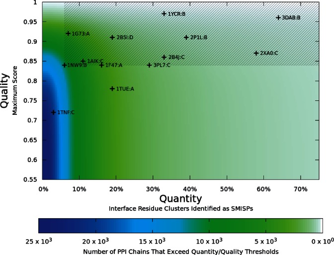
A density plot of the quantity and quality of the predicted SMISPs of all the complexes in our non-redundant set of PPIs. 95% of PPIs have at least one predicted SMISP, but significantly fewer have a significant quantity of highly ranked SMISPs. PPIs with known structure and known inhibitors from Figure 2 and Table 1 are shown plotted at their maximal quantity/quality. These complexes are clearly biased towards the less populated, high quality, high quantity region of the plot. Of the 13 complexes, 11 are contained within the shaded area defined by a minimum quantity of 6% and a minimum quality of 0.84. 10,920 chains (40%) and 5,757 PPIs (48%) of the non-redundant PDB subset are contained within this region. Since these structures share the same quality/quantity profile as structures with known inhibitors, we predict that they are accessible to small-molecule inhibitor design.
A quantity/quality threshold of (≥6%, ≥0.84), shown shaded in Figure 4, selects 11 of the 13 complexes with known inhibitors. The remaining two complexes, HPV E1/E2 and TNF-α from Figures 3g and h, were the two cases where the predicted SMISP failed to identify the binding site of the inhibitor due to conformational changes of the protein receptor. Since this is the strictest threshold that captures all the PPIs where the predicted SMISPs correctly identify the binding site of the inhibitor, we predict that complexes within this threshold are likely susceptible to small-molecule inhibition through the chemical mimicry of a small set of interface residues. Nearly half, 48%, of all the PPIs in our dataset fall within this threshold. Of course, this estimate does not include the potential to design allosteric inhibitors. Additionally, our analysis is based on existing structures and therefore cannot predict the susceptibility of PPIs to new mechanisms of inhibition.
The quality and quantity thresholds computed for each PPI chain define a partial order, where one chain is better than another if it has both a higher score and a greater quantity. We use this partial order to rank every PPI chain in our dataset and provide this ranking in the Supplementary Data.
4 DISCUSSION
PPIs are an emerging class of biological targets that have been poorly addressed by high throughput screening (Macarron, 2006). The steadily increasing amount of PPI structural information makes structure-based rational design one attractive alternative. The interactions of the complex itself provide a natural starting point as long as the most favorable interactions can be effectively identified. Previous work has largely focused on identifying individual hotspots, i.e. single residues that contribute a significant portion of the free energy of the complex. We have built upon this previous work to address the problem of finding an entire set of residues that, as a unit, identify a binding site that is susceptible to small-molecule inhibition. Our automated structural bioinformatics method learns both scoring (SVM-based) and filtering (rule-based) classifiers for identifying these sites.
A novel aspect of our method is that we use the structure of PPI complexes and known binders at the PPI interface to create our training set. SMISPs are identified purely from the steric overlap of small-molecule binders and the PPI structure. This results in a less quantitative assessment of training examples compared to using alanine scanning results. However, our structure-based approach has several advantages. The existence of a high-affinity ligand at the protein interface is more relevant to our goal of identifying small-molecule starting points. Alanine scanning may identify hot spots for reasons that are not relevant to inhibition, such as the residue's contribution to protein stability. Additionally, the ΔΔG does not include any backbone contributions, which may be important for small molecule design. Our structure-based method naturally identifies groups of co-located residues, SMISPs, as opposed to single, potentially isolated hot spot residues. Finally, our method benefits from the rapidly increasing number of available protein structures, exemplified by the PDB.
We use a standard SVM classifier for ranking SMISPs, but also find that simple thresholding rules provide an easily interpretable alternative classifier with accuracy similar to more sophisticated techniques. Unlike previous work that relied on a subjective evaluation of histograms to set rule thresholds (Tuncbag et al., 2009), our exhaustive rule classifier uses information theoretic techniques to automatically identify the optimal classification rules from the training set.
Our approach correctly predicts the binding sites and, to a lesser extent, the interactions of several known PPI inhibitors. Perhaps more interestingly, the application of our classifiers to a non-redundant subset of the PDB containing more than 12,000 complexes reveals that nearly half the complexes contain at least one chain that has a similar distribution of predicted SMISPs as complexes with known inhibitors. This suggests that PPIs may be substantially more susceptible to small-molecule inhibition than indicated by the current distribution of pharmaceutical targets (Paolini et al., 2006). The historical bias against PPI targets present in existing compound libraries makes structure-based rational design a logical paradigm for developing PPI inhibitors. The SMISPs identified using our approach and available from http://pocketquery.csb.pitt.edu provide an immediate computational hypothesis to initiate such efforts which have the potential to ultimately culminate in the design of novel therapeutics.
Funding: National Institute of Health [1R21GM087617, R01GM097082].
Conflict of Interest: none declared.
REFERENCES
- Altschul S. F., Gish W., Miller W., Myers E. W., Lipman D. J. Basic local alignment search tool. J. Mol. Biol. 1990;215(3):403–410. doi: 10.1016/S0022-2836(05)80360-2. [DOI] [PubMed] [Google Scholar]
- An J., Totrov M., Abagyan R. Pocketome via comprehensive identification and classification of ligand binding envelopes. Mol. Cell. Proteomics. 2005;4(6):752. doi: 10.1074/mcp.M400159-MCP200. [DOI] [PubMed] [Google Scholar]
- Batuwita R., Palade V. Efficient resampling methods for training support vector machines with imbalanced datasets. Neural Networks (IJCNN), The 2010 International Joint Conference on IEEE Computer Society. 2010:1–8. [Google Scholar]
- Bordner A. J., Abagyan R. Statistical analysis and prediction of protein–protein interfaces. Proteins: Struct, Funct, Bioinf. 2005;60(3):353–366. doi: 10.1002/prot.20433. [DOI] [PubMed] [Google Scholar]
- Bourgeas R., Basse M.-J., Morelli X., Roche P. Atomic analysis of protein–protein interfaces with known inhibitors: The 2p2i database. PLoS One. 2010;5(3):e9598. doi: 10.1371/journal.pone.0009598. [DOI] [PMC free article] [PubMed] [Google Scholar]
- Brenke R., Kozakov D., Chuang G. Y., Beglov D., Hall D., Landon M. R., Mattos C., Vajda S. Fragment-based identification of druggable hot spots of proteins using fourier domain correlation techniques. Bioinformatics. 2009;25(5):621. doi: 10.1093/bioinformatics/btp036. [DOI] [PMC free article] [PubMed] [Google Scholar]
- Bromberg Y., Rost B. Comprehensive in silico mutagenesis highlights functionally important residues in proteins. Bioinformatics. 2008;24(16):i207. doi: 10.1093/bioinformatics/btn268. [DOI] [PMC free article] [PubMed] [Google Scholar]
- Brooks B. R., Bruccoleri R. E., Olafson B. D. Charmm: A program for macromolecular energy, minimization, and dynamics calculations. Journal of computational chemistry. 1983;4(2):187–217. [Google Scholar]
- Camacho C., Zhang C. FastContact: rapid estimate of contact and binding free energies. Bioinformatics. 2005;21(10):2534. doi: 10.1093/bioinformatics/bti322. [DOI] [PubMed] [Google Scholar]
- Chan D., Chutkowski C., Kim P. Evidence that a prominent cavity in the coiled coil of HIV type 1 gp41 is an attractive drug target. PNAS. 1998;95(26):15613. doi: 10.1073/pnas.95.26.15613. [DOI] [PMC free article] [PubMed] [Google Scholar]
- Cho K., Kim D., Lee D. A feature-based approach to modeling protein–protein interaction hot spots. Nucleic Acids Res. 2009;37(8):2672. doi: 10.1093/nar/gkp132. [DOI] [PMC free article] [PubMed] [Google Scholar]
- Christ F., Voet A., Marchand A., Nicolet S., Desimmie B. A., Marchand D., Bardiot D., Van der Veken N. J., Van Remoortel B., Strelkov S. V. Rational design of small-molecule inhibitors of the ledgf/p75-integrase interaction and hiv replication. Nature Chemical Biology. 2010;6(6):442–448. doi: 10.1038/nchembio.370. [DOI] [PubMed] [Google Scholar]
- Clackson T., Wells J. A. A hot spot of binding energy in a hormone-receptor interface. Science. 1995;267(5196):383–386. doi: 10.1126/science.7529940. 10.1126/science.7529940. [DOI] [PubMed] [Google Scholar]
- Darnell S., Page D., Mitchell J. An automated decision-tree approach to predicting protein interaction hot spots. Proteins: Struct. Funct. Bioinf. 2007;68(4):813–823. doi: 10.1002/prot.21474. [DOI] [PubMed] [Google Scholar]
- Davis F. P., Sali A. The overlap of small molecule and protein binding sites within families of protein structures. PLoS Computational Biology. 2010;6(2):e1000668. doi: 10.1371/journal.pcbi.1000668. [DOI] [PMC free article] [PubMed] [Google Scholar]
- Dömling A. Small molecular weight protein–protein interaction antagonists–an insurmountable challenge? Curr. Opin. Chem. Biol. 2008;12(3):281–291. doi: 10.1016/j.cbpa.2008.04.603. [DOI] [PubMed] [Google Scholar]
- Fuller J., Burgoyne N., Jackson R. Predicting druggable binding sites at the protein–protein interface. Drug discovery today. 2009;14(3-4):155–161. doi: 10.1016/j.drudis.2008.10.009. [DOI] [PubMed] [Google Scholar]
- Guney E., Tuncbag N., Keskin O., Gursoy A. HotSprint: database of computational hot spots in protein interfaces. Nucleic Acids Res. 2008;36(suppl 1):D662. doi: 10.1093/nar/gkm813. [DOI] [PMC free article] [PubMed] [Google Scholar]
- Hajduk P. J., Huth J. R., Tse C. Predicting protein druggability. Drug Discovery Today. 2005;10:1675–1682. doi: 10.1016/S1359-6446(05)03624-X. doi:10.1016/S1359-6446(05)03624-X. [DOI] [PubMed] [Google Scholar]
- Henrich S., Salo-Ahen O., Huang B., Rippmann F., Cruciani G., Wade R. Computational approaches to identifying and characterizing protein binding sites for ligand design. Journal of Molecular Recognition. 2010;23(2):209–219. doi: 10.1002/jmr.984. [DOI] [PubMed] [Google Scholar]
- Higueruelo A. P., Schreyer A., Bickerton G. R. J., Pitt W. R., Groom C. R., Blundell T. L. Atomic interactions and profile of small molecules disrupting protein–protein interfaces: Timbal database. Chem. Biol. Drug Des. 2009;74(5):457–467. doi: 10.1111/j.1747-0285.2009.00889.x. [DOI] [PubMed] [Google Scholar]
- Hu L., Benson M. L., Smith R. D., Lerner M. G., Carlson H. A. Binding moad (mother of all databases) Proteins: Struct. Funct. Bioinf. 2005;60(3):333–340. doi: 10.1002/prot.20512. [DOI] [PubMed] [Google Scholar]
- Jochim A. L., Arora P. S. Systematic analysis of helical protein interfaces reveals targets for synthetic inhibitors. ACS Chemical Biology. 2010;5(10):919–923. doi: 10.1021/cb1001747. [DOI] [PMC free article] [PubMed] [Google Scholar]
- Keskin O., Ma B., Nussinov R. Hot regions in protein–protein interactions: the organization and contribution of structurally conserved hot spot residues. J. Mol. Biol. 2005;345(5):1281–1294. doi: 10.1016/j.jmb.2004.10.077. [DOI] [PubMed] [Google Scholar]
- Kortemme T., Kim D., Baker D. Computational alanine scanning of protein–protein interfaces. Sci STKE. 2004;2004(219):l2. doi: 10.1126/stke.2192004pl2. [DOI] [PubMed] [Google Scholar]
- Larkin M. A., Blackshields G., Brown N. P., Chenna R., McGettigan P. A., McWilliam H., Valentin F., Wallace I. M., Wilm A., Lopez R. Clustal w and clustal x version 2.0. Bioinformatics. 2007;23(21):2947. doi: 10.1093/bioinformatics/btm404. [DOI] [PubMed] [Google Scholar]
- Lichtarge O., Bourne H. R., Cohen F. E. An evolutionary trace method defines binding surfaces common to protein families. J. Mol. Biol. 1996;257(2):342–358. doi: 10.1006/jmbi.1996.0167. [DOI] [PubMed] [Google Scholar]
- Lin J., Chen J., Elenbaas B., Levine A. J. Several hydrophobic amino acids in the p53 amino-terminal domain are required for transcriptional activation, binding to mdm-2 and the adenovirus 5 e1b 55-kd protein. Genes Dev. 1994;8(10):1235. doi: 10.1101/gad.8.10.1235. [DOI] [PubMed] [Google Scholar]
- Lise S., Archambeau C., Pontil M., Jones D. Prediction of hot spot residues at protein–protein interfaces by combining machine learning and energy-based methods. BMC bioinformatics. 2009;10(1):365. doi: 10.1186/1471-2105-10-365. [DOI] [PMC free article] [PubMed] [Google Scholar]
- Liu S., Wu S., Jiang S. HIV entry inhibitors targeting gp41: from polypeptides to small-molecule compounds. Curr. Pharm. Des. 2007;13(2):143–162. doi: 10.2174/138161207779313722. [DOI] [PubMed] [Google Scholar]
- Liu T., Lin Y., Wen X., Jorissen R. N., Gilson M. K. Bindingdb: a web-accessible database of experimentally determined protein-ligand binding affinities. Nucleic Acids Res. 2006;35:D198. doi: 10.1093/nar/gkl999. [DOI] [PMC free article] [PubMed] [Google Scholar]
- Macarron R. Critical review of the role of hts in drug discovery. Drug Discovery Today. 2006;11:277–279. doi: 10.1016/j.drudis.2006.02.001. [DOI] [PubMed] [Google Scholar]
- Mayrose I., Graur D., Ben-Tal N., Pupko T. Comparison of site-specific rate-inference methods for protein sequences: Empirical bayesian methods are superior. Molecular biology and evolution. 2004;21(9):1781. doi: 10.1093/molbev/msh194. [DOI] [PubMed] [Google Scholar]
- Meireles L., Dömling A. S., Camacho C. J. Anchor: a web server and database for analysis of protein–protein interaction binding pockets for drug discovery. Nucleic Acids Res. 2010;38:W407. doi: 10.1093/nar/gkq502. [DOI] [PMC free article] [PubMed] [Google Scholar]
- Moreira I., Fernandes P., Ramos M. Hot spots: A review of the protein–protein interface determinant amino-acid residues. Proteins: Struct. Funct. Bioinf. 2007;68(4):803–812. doi: 10.1002/prot.21396. [DOI] [PubMed] [Google Scholar]
- Ofran Y., Rost B. Protein–protein interaction hotspots carved into sequences. PLoS. Comput. Biol. 2007;3(7):e119. doi: 10.1371/journal.pcbi.0030119. [DOI] [PMC free article] [PubMed] [Google Scholar]
- Paolini G., Shapland R., van Hoorn W., Mason J., Hopkins A. Global mapping of pharmacological space. Nature biotechnology. 2006;24(7):805–815. doi: 10.1038/nbt1228. [DOI] [PubMed] [Google Scholar]
- Pérot S., Sperandio O., Miteva M. A., Camproux A. C., Villoutreix B. O. Druggable pockets and binding site centric chemical space: a paradigm shift in drug discovery. Drug discovery today. 2010;15:656–667. doi: 10.1016/j.drudis.2010.05.015. [DOI] [PubMed] [Google Scholar]
- Popowicz G., Dömling A., Holak T. The Structure-Based Design of Mdm2/Mdmx–p53 Inhibitors Gets Serious. Angew. Chem. Int. Ed. 2011;50(12):2680–2688. doi: 10.1002/anie.201003863. [DOI] [PMC free article] [PubMed] [Google Scholar]
- Rajamani D., Thiel S., Vajda S., Camacho C. J. Anchor residues in protein–protein interactions. PNAS. 2004;101(31):11287. doi: 10.1073/pnas.0401942101. [DOI] [PMC free article] [PubMed] [Google Scholar]
- Rijnbeek P. R., Kors J. A. Finding a short and accurate decision rule in disjunctive normal form by exhaustive search. Machine learning. 2010;80(1):33–62. [Google Scholar]
- Stewart K. D., Huth J. R., Ng T. I., McDaniel K., Hutchinson R. N., Stoll V. S., Mendoza R. R., Matayoshi E. D., Carrick R., Mo H. M. Non-peptide entry inhibitors of hiv-1 that target the gp41 coiled coil pocket. Bioorg. Med. Chem. Lett. 2010;20(2):612–617. doi: 10.1016/j.bmcl.2009.11.076. [DOI] [PubMed] [Google Scholar]
- Tuncbag N., Gursoy A., Keskin O. Identification of computational hot spots in protein interfaces: combining solvent accessibility and inter-residue potentials improves the accuracy. Bioinformatics. 2009;25(12):1513. doi: 10.1093/bioinformatics/btp240. [DOI] [PubMed] [Google Scholar]
- Valdar W. S. J. Scoring residue conservation. Proteins: Struct Funct Bioinf. 2002;48(2):227–241. doi: 10.1002/prot.10146. [DOI] [PubMed] [Google Scholar]
- Wang R., Fang X., Lu Y., Yang C. Y., Wang S. The pdbbind database: methodologies and updates. Journal of medicinal chemistry. 2005;48(12):4111–4119. doi: 10.1021/jm048957q. [DOI] [PubMed] [Google Scholar]
- Weisel M., Proschak E., Schneider G. PocketPicker: analysis of ligand binding-sites with shape descriptors. Chem. Cent. J. 2007;1(7):1–17. doi: 10.1186/1752-153X-1-7. [DOI] [PMC free article] [PubMed] [Google Scholar]
- Wells J., McClendon C. Reaching for high-hanging fruit in drug discovery at protein–protein interfaces. Nature. 2007;450(7172):1001–1009. doi: 10.1038/nature06526. [DOI] [PubMed] [Google Scholar]
- Wu C. H., Apweiler R., Bairoch A., Natale D. A., Barker W. C., Boeckmann B., Ferro S., Gasteiger E., Huang H., Lopez R. The universal protein resource (uniprot): an expanding universe of protein information. Nucleic Acids Res. 2006;34(suppl 1):D187. doi: 10.1093/nar/gkj161. [DOI] [PMC free article] [PubMed] [Google Scholar]
- Wu T. F., Lin C. J., Weng R. C. Probability estimates for multi-class classification by pairwise coupling. JMLR. 2004;5:975–1005. [Google Scholar]
- Zhu X., Mitchell J. C. Kfc2: A knowledge-based hot spot prediction method based on interface solvation, atomic density, and plasticity features. Proteins: Struct. Funct. Bioinf. 2011;79(9):2671–2683. doi: 10.1002/prot.23094. [DOI] [PubMed] [Google Scholar]