

Abstract
Quantification of chemical toxicity continues to be generally based on measured external concentrations. Yet, internal chemical concentrations have been suggested to be a more suitable parameter. To better understand the relationship between the external and internal concentrations of chemicals in fish, and to quantify internal concentrations, we compared three toxicokinetic (TK) models with each other and with literature data of measured concentrations of 39 chemicals. Two one-compartment models, together with the physiologically based toxicokinetic (PBTK) model, in which we improved the treatment of lipids, were used to predict concentrations of organic chemicals in two fish species: rainbow trout (Oncorhynchus mykiss) and fathead minnow (Pimephales promelas). All models predicted the measured internal concentrations in fish within 1 order of magnitude for at least 68% of the chemicals. Furthermore, the PBTK model outperformed the one-compartment models with respect to simulating chemical concentrations in the whole body (at least 88% of internal concentrations were predicted within 1 order of magnitude using the PBTK model). All the models can be used to predict concentrations in different fish species without additional experiments. However, further development of TK models is required for polar, ionizable, and easily biotransformed compounds.
Introduction
Toxicokinetic Models in Risk Assessment
Environmental regulations require comprehensive testing and risk assessment before a chemical can be approved for use. In ecological risk assessment of chemicals in water, fish play a very important role, being the only vertebrate representative of freshwater systems.1 Quantification of chemical toxicity is generally based on measurements of external exposure; however, in order to understand, interpret, and extrapolate toxicological effects, internal concentrations of chemicals are more suitable.2,3 For this reason, we need to understand the relationship between the external and internal concentration of chemicals in fish. Further, in silico (model) predictions of concentrations in fish (i.e., bioconcentration) could reduce or replace the need for in vivo (animal) experiments which are costly and involve large numbers of fish.
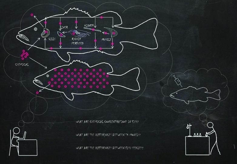
Toxicokinetics captures information about uptake, distribution, biotransformation, and elimination of a toxicant in an organism, and is important in risk assessment because a chemical needs to enter the organism and reach the site of action in order to elicit an effect.4−6 Toxicokinetic models, when combined with toxicodynamic models, can predict toxic effects on organisms. In addition, they can be applied to time-variable concentrations, a wide-range of chemicals, and to extrapolation between different species and from in vitro to organism scale.7−10 Provided that the necessary physiological parameters are known, generally, two groups of TK models can be distinguished: models based on a one-compartment assumption, according to which the chemical concentration is the same throughout the organism, and multicompartment models, which assume that chemical concentrations may differ among various organs and tissues. Thus, the multicompartment approach, apart from chemical uptake, biotransformation, and elimination, also describes the movement of chemicals among various compartments that usually represent different organs.
A comparison of toxicokinetic models is required so that the most suitable model can be chosen for a given question or condition. A comparison of different model structures was presented by Landrum and co-workers11 who described advantages and disadvantages of equilibrium and kinetic models. Also, Mackay and Fraser12 presented a review of bioaccumulation models in which they compared the structure of empirical and mechanistic approaches. Both these reviews compared different models based on their underlying assumptions and model structures; they did not compare model predictions with measured data. To our knowledge there is no study using a wide scope of chemicals to test model performance on independent data.
Problem Formulation
One-compartment models can be perceived as simple, because they require only a few physiological parameters and simulate one compartment only. Consequently they can only be used to estimate a chemical concentration in the whole body of an organism. On the other hand, a multicompartment model, e.g., the physiologically based toxicokinetic (PBTK) model developed for fish by Nichols and co-workers,13 may be viewed as more complex than one-compartment models because it requires more physiological data and simulates multiple compartments. This model is generally used when a chemical’s concentration in a specific organ or tissue plays an important role, e.g., when the tissue or organ is the dominant site of action. This raises the question of whether the PBTK model is a suitable model for predicting chemical concentration in both organism tissues and whole body. If so, another important issue is whether it is worth using the more complex PBTK model with many parameters to predict whole body chemical concentrations, or whether the simpler one-compartment approach with only a few parameters suffices. Thus, we aim to quantify model performance in predicting fish internal concentrations in order to explain model differences and to guide model selection.
Study Overview
In the present study, we compared predictions of one PBTK and two one-compartment models with measured concentrations of organic chemicals in rainbow trout (Oncorhynchus mykiss) and fathead minnow (Pimephales promelas), available from the literature and databases. Differences between models were explained based on a sensitivity analysis of each approach. In addition, we improved the treatment of lipids in the PBTK model.
Materials and Methods
Method
Two one-compartment models (A14 and B15) and the PBTK13 model were used to simulate internal concentrations of chemicals in fish. Only respiratory uptake routes were considered for both model types and they were described by mass-balance differential equations. None of the models included chemical biotransformation in fish. Chemical concentrations in water were used as model inputs in order to calculate chemical concentrations in the whole fish body. Tissue-specific concentrations were not taken into account, even for the PBTK approach, because a comparison with one-compartment models or whole body residue data is not meaningful.
Origin of Measured Internal Concentrations
Measured internal concentrations of organic chemicals in rainbow trout and fathead minnow were found using the TOXRES Database16 and by searching the peer-reviewed literature in the Scopus online database (see details about search method in Supporting Information). We used only references with exposure via water and containing all required data, i.e., fish weight, chemical concentration in water, measured internal concentration, exposure time, water temperature, and dissolved oxygen concentration in water (SI Tables S1–S3).
In total, measured internal concentrations for 23 different organic chemicals (39 different chemical concentrations in water) for rainbow trout and for 24 different chemicals (68 different chemical concentrations in water) for the fathead minnow were taken from the TOXRES Database and studies identified in the Scopus reference database (Tables S2–S3). For eight chemicals, internal concentrations were available for both fish species.
Internal concentrations of phenol and 2,4,5-trichlorophenol in the fathead minnow17 had already been used in the original development of model B for calibration.15 For this reason, we show these two chemicals in graphs; however, we did not take them into consideration in the statistical model evaluation. To our knowledge, none of the other internal concentrations presented have been used to calibrate any of the models studied here.
Model Design, Formulation, and Description
One-Compartment Approach
We chose two one-compartment approaches to predict internal concentrations of organic chemicals in fish. Common to both models is that they use octanol–water partition coefficients to quantify partitioning, and that they assume that the chemical is homogeneously circulated within the organism.18 According to the one-compartment concept, a chemical which enters the fish is distributed instantaneously and equally. This concept can be described with the following equation:11,15,19
| 1 |
where Cint(t) is the internal chemical concentration (amount × mass–1), Cw(t) is the chemical concentration in the water (amount × volume–1), kin is the uptake rate constant (volume × mass–1 × time–1), and kout is the elimination rate constant (time–1).
The first model, herein referred to as the one-compartment model A, was developed to predict the bioaccumulation processes of organic chemicals in aquatic ecosystems with the aim of providing data on site-specific toxicant concentrations and associated bioconcentration, bioaccumulation, and biota–sediment accumulation factors in organisms of aquatic food webs.14 Thus, this model uses a small number of chemical, site-specific, and organism parameters. According to Arnot and Gobas,14 it is possible to describe the exchange of nonionic organic chemicals between the organism and its environment using a single equation for various aquatic animals.
The second toxicokinetic approach, referred to as one-compartment model B, describes the accumulation kinetics of organic chemicals as a function of the octanol–water partition coefficient (Kow), as well as the lipid content, weight, and trophic level of the species.15 This model is driven by both species and chemical properties and its goal was to explain differences in accumulation between various substances and between species. According to Hendriks et al.,15 this model may be used in risk assessment, both for predicting the equilibrium accumulation potential and for estimating nonequilibrium kinetics.
Physiologically Based Toxicokinetic Model (PBTK)
The physiologically based multicompartment model for fish8,9,13 was used and further developed by incorporating a relationship between lipid fractions in the whole body and the volume of fat compartment (SI eqs S20–S22). That relationship was suggested by Nichols and colleagues20 who assumed that the lipid content of lean tissue (consisting of all tissues except adipose fat) is independent of whole body lipid content. Support for this assumption is provided by examining blood lipid content values reported by Bertelsen et al.21 for several fish species. In their study, the extreme case was represented by channel catfish, which tend to have a low whole-body lipid content. However, despite the “lean” nature of these animals, the blood lipid content in catfish was essentially identical to that of trout. Thus we set the lipid content of the lean tissues to the values derived by Bertelsen et al.21 while the volume of the adipose fat compartment was adjusted to achieve the required whole body lipid content. Note, that this simplification will not work for the extreme situation when the whole body lipid content is lower than the assumed lipid content of lean tissues. According to SI eq S22, the volume of the fat compartment would then be below zero. However, in the experiments modeled here, this simplified relationship is sufficient.
The PBTK model for rainbow trout takes into account five different compartments (liver, kidney, fat, richly perfused tissues, and poorly perfused tissues). Due to the lack of data characterizing the kidney, a four-compartment (liver, fat, richly perfused tissues, and poorly perfused tissues) PBTK model was created for the fathead minnow. The model assumes that all parts of the whole body belong to one of the compartments, so the sum of the weight or volume of all compartments is equal to the weight or volume of the whole organism. The amount of the chemical in each compartment is calculated based on eq 2,13 and the total amount of the chemical can be used for calculating the internal concentration in the whole fish body (eq 3).
| 2 |
where Ai(t) is the amount of chemical in compartment i (amount), Qi is the arterial blood flow to compartment i (volume × time–1), Cart(t) is the chemical concentration in arterial blood (amount × volume–1), Cvi(t) is the chemical concentration in venous blood after compartment i (amount × volume–1), and t is time.
| 3 |
where Cint(t) is the internal chemical concentration (amount × mass–1), ∑Ai(t) is the amount of chemical in all compartments (amount), and BW is the body wet weight (mass).
Detailed model descriptions and parameters for running the models are presented in SI.
Model Calibration
In this study, models were used as calibrated by their original authors. The one-compartment model A was calibrated with measured field bioaccumulation factors, while the one-compartment model B was calibrated with measured values of uptake and elimination rates from laboratory experiments. In general, the PBTK model does not have to be calibrated as it is based on physiological parameters and processes that can be measured directly. However, some parts of this model, e.g., partition coefficients between tissues and blood were calibrated separately by their original authors (all model equations and parameters are available in the SI).
Model Sensitivity Analysis
In the model sensitivity analysis, we took into account the impact of changes of four parameters (log KOW, fish weight, water temperature, and lipid content in fish) on model predictions. The minimum and maximum values of the possible parameter range for each fish species were taken from the literature. The sensitivity analysis was carried out by varying each parameter separately (one at a time sensitivity analysis, 99 runs each).
Model Implementation
All simulations and sensitivity analyses were carried out using ModelMaker software, version 4.0, developed and published by Cherwell Scientific Ltd. (Oxford, UK). In addition, all calculations were also checked in Mathcad 14 (Parametric Technology Corporation, Needham, MA).
Quantification of Model Performance
To evaluate and compare the TK models, we have used the following three methods:
-
(i)Coefficient of determination (r2), here, refers to the square of the correlation coefficient between measured and modeled values, and quantifies the fraction of the variability in the data that is explained by the model (eq 4, based on the FOCUS guidance document22). The closer r2 is to 1, the better the model predicts the measured internal concentrations.
where n is the total number of paired observations (P, O), Pi is the ith value of the predicted internal concentration (with i = 1,2,...,n), Oi is the ith value of the measured internal concentration (with i = 1,2,...,n), P̅ is the mean of all values for predicted internal concentrations, and O̅ is the mean of all values for measured internal concentrations.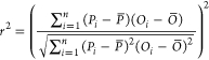
4 -
(ii)Factor_10 (or Factor_5, see eq 5) quantifies internal chemical concentrations that are predicted with differences between measured and predicted values equal to or smaller than 1 order of magnitude (or five times). This can be seen as a practitioners view of model performance. If Factor_10 or Factor_5 is closer to 100%, the model is in better agreement with the measured internal concentrations.
where Oi is the ith value of the measured internal concentration (with i = 1,2,...,n), Pi is the ith value of the predicted internal concentration (with i = 1,2,...,n), and n is the total number of paired observations (P, O).
5 -
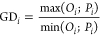
(iii)General distance (GD) evaluates the model accuracy (i.e., agreement with absolute values of measured data). This approach characterizes over- or under-prediction of measured internal concentrations by the model by quantifying the distance between measured and predicted values (eqs 6 and 7). The closer GD is to 1, the better is the model in agreement with the measured internal concentrations.
6
where GDi is the ith value of General Distance (with i = 1,2,...,n), Oi is the ith value of the measured internal concentration (with i = 1,2,...,n), Pi is the ith value of the predicted internal concentration (with i = 1,2,...,n), and n is the total number of paired observations (P, O).
7
Results and Discussion
Rainbow Trout
For rainbow trout, differences between the TK models were small (Figure 1 and Table 1) and r2 values for the one-compartment models A and B and the PBTK model were 0.76, 0.80, and 0.78, respectively. However, overall, the distance between the predicted and measured values of internal concentrations was the smallest for the PBTK model (GD was equal to 3.7, 3.73, and 3.54 for the one-compartment A, the one-compartment B, and the PBTK model, respectively).
Figure 1.

Comparison of predicted internal concentrations of chemicals (based on one-compartment A [○], one-compartment B [+], and PBTK [⧫] models) and measured internal concentrations in (1.1) rainbow trout and (1.2) fathead minnow; circles: “outlier” chemicals explained in text; green: hexachlorobenzene (see also black and white graph in SI Figure S2).
Table 1. Statistical Analysis of TK Models for Both Fishes (Rainbow Trout: 23 Chemicals, 39 Data Points; Fathead Minnow: 24 Chemicals, 68 Data Points)a.
| rainbow trout |
fathead minnow |
|||||
|---|---|---|---|---|---|---|
| one-compartment |
one-compartment |
|||||
| statistical method | A | B | PBTK | A | B | PBTK |
| coefficient of determination (r2), ― | 0.76 | 0.80 | 0.78 | 0.64 | 0.77 | 0.73 |
| factor_10, % | 90 | 95 | 95 | 68 | 76 | 88 |
| factor_5, % | 85 | 82 | 77 | 62 | 61 | 80 |
| general distance (GD), ― | 3.7 | 3.73 | 3.54 | 29 | 25.3 | 16.2 |
Italics indicate the best agreement between the model and measured data.
Fathead Minnow
Not all chemicals’ internal concentrations in fathead minnow were predicted well using the TK models (Figure 1). For one internal concentration of hexachlorobenzene, the PBTK model underestimated the measured value by a factor of over 20 (predicted: 0.014 μg/g, observed: 0.3014 μg/g). However, in the same experiment, various chemical concentrations were taken into account (green points in Figure 1), and only for the lowest concentration, the PBTK model underestimated results by such a large margin.
Other chemicals for which measured internal concentrations were underestimated by the TK models by more than a factor of 10 were phenol, 2,4,5-trichlorophenol (for the PBTK model), and 4-nitrophenol. A possible explanation is that these are polar organic compounds, whose partitioning behavior cannot be well characterized by means of octanol–water partition coefficients.23 Yet, an internal concentration of the polar compound, 4-nitrophenol, was also predicted in rainbow trout (SI Table S1) but without any underestimation (Figure 1). It was noticed by Call and co-workers17 that phenolic compounds are much more bioconcentrated in fathead minnow than in rainbow trout. In general, the bioconcentration of weak acids, such as 4-nitrophenol, can differ due to water pH.24 However, in the experiments considered here, the water pH values were not sufficiently different to account for the difference in bioconcentration between species, but we cannot totally exclude its influence as pH might differ also at the actual site of uptake (e.g., gill surface).
In the present study, apart from phenol, 2,4,5-trichlorophenol, and 4-nitrophenol, only C12LAS (sodium dodecylbenzene sulfonate) can be classified as a polar compound. However, unlike the above-mentioned polar toxicants, measured internal concentrations of this chemical were overestimated by all three TK approaches. C12LAS is a surfactant, which is amphiphilic in nature, with a polar head and a nonpolar chain, and if the system is not constantly mixed, this chemical tends to concentrate at interphases (e.g., water/air; water/plastic).25 For this reason, there are problems in estimating how much C12LAS in water is available for an organism (bioavailability), which may result in very low measurements of internal concentrations in comparison with apparent concentrations in water.
For hexachlorocyclopentadiene, internal concentrations were also overestimated by the TK models. Based on the octanol–water partition coefficient of hexachlorocyclopentadiene (log KOW = 5.04; Table S3), this chemical should bioconcentrate. According to EPI Suite, the calculated bioconcentration factor (BCF) is equal to 3606 while with EUSES, a BCF of 3800 was estimated;26 however, experiments carried out by Podowski and colleagues27 have shown that this chemical is hardly bioconcentrated in fish, likely due to biotransformation. According to Spehar and co-workers,28 the BCF of hexachlorocyclopentadiene for fathead minnow is 11. Thus, predicting internal concentrations of hexachlorocyclopentadiene, without taking its biotransformation into account, causes overestimation by TK models.
According to the GD (Table 1) for fathead minnow, all three approaches overestimated internal concentrations by more than 1 order of magnitude on average. Moreover, the correlations of model predictions and data were lower than for rainbow trout (r2 for the one-compartment A, the one-compartment B, and the PBTK models were equal to 0.64, 0.77, and 0.73, respectively). The difference in agreement between the modeled and measured data, indicated by factor_10 (equal to 68–88%) and GD (16.2–29) methods, can be explained by the “outlier” group of chemicals (described above) which was included in the calculation of both statistical methods. Not many chemicals belong to this “outlier” group (which influences the factor_10). For most of these, however, TK models over- or underestimated measured internal concentrations much more than by a factor of 10 (which influences the GD).
Comparison of Rainbow Trout and Fathead Minnow Results
Differences between results for rainbow trout and fathead minnow can be caused by several factors. First, different data sets were used for each fish species. From the “outlier” group of chemicals (chemicals for which internal concentration was over- or underestimated by more than a factor of 10—discussed above) for the fathead minnow, only hexachlorobenzene and 4-nitrophenol were also used in the TK models for rainbow trout. However, it was decided not to compare predicted internal concentrations of 4-nitrophenol in both fishes, due to the presumed impact of its polar nature and water pH on bioavailability (see Fathead Minnow section). For the other chemicals from this group (i.e., phenol, 2,4,5-trichlorophenol, hexachlorocyclopentadiene, and C12LAS), no data on internal concentrations in rainbow trout were available. The comparison of TK models was made for chemicals that were used in both fishes (Tables S2 and S3 and Figure 2).
Figure 2.

Comparison of TK models: One-compartment A (○), one-compartment B (+), and PBTK (⧫), for the same chemicals for rainbow trout and fathead minnow (8 chemicals, 45 data points); blue: results for rainbow trout, green: results for fathead minnow (see also black and white graph in SI Figure S3).
According to Figure 2, results demonstrate a clear relationship between predicted and measured internal concentrations for all models and for both fishes. This indicates that the difference between the statistical results for rainbow trout and fathead minnow was caused mainly by the “outlier” group of chemicals used in predicting internal concentrations in fathead minnow. However, we noticed that both the values of the coefficients of determination and the factor_5 are now much lower for rainbow trout than for fathead minnow (Table 2). Additionally, the GD between predicted and measured internal concentrations increased for rainbow trout in relation to GD for all chemicals in this species (Table 1), while for fathead minnow, the GD is now much lower than it was for all chemicals. The difference between the results for both fish species might be due to two main reasons. The first of them results from the fact that five (out of 12) of the measured internal concentrations used in rainbow trout came from the same study,29 and all measured internal concentrations taken from this reference were underestimated by all TK models used. The second reason is that different exposure times were used in the experiments. Generally, fathead minnow were not exposed to chemicals for short durations (the shortest exposure time: 28 days; average: 32 days) compared to rainbow trout (the shortest exposure time: < 3 h; average: 70 days). Biotransformation may modify internal concentrations differently under short or long exposure times. In addition, if steady-state conditions occur, the difference between TK models might be smaller than under non-steady-state conditions.
Table 2. Statistical Analysis of TK Models for Selected Chemicals in Both Fishes (8 Chemicals, Rainbow Trout: 12 Data Points; Fathead Minnow: 33 Data Points)a.
| rainbow trout |
fathead minnow |
|||||
|---|---|---|---|---|---|---|
| one-compartment |
one-compartment |
|||||
| statistical method | A | B | PBTK | A | B | PBTK |
| coefficient of determination (r2), ― | 0.26 | 0.60 | 0.64 | 0.85 | 0.85 | 0.76 |
| factor_10, % | 85 | 85 | 100 | 81 | 86 | 97 |
| factor_5, % | 69 | 77 | 69 | 81 | 78 | 89 |
| general distance (GD), ― | 5.03 | 4.67 | 4.53 | 4.8 | 3.8 | 3.5 |
Italics indicate the best agreement between the model and measured data.
Model Sensitivity Analysis
Differences between TK model predictions in relation to exposure times are shown in Figure 3. Model-based predictions differ during short-term exposure (shorter than 10 days, Figure 3) more than during long-term exposure (Figure 3 and 3). This disparity between approaches can be explained by a sensitivity analysis of the model. In Figure 4, the impact of log KOW and lipid fractions on model performance is presented. Sensitivity analysis of other model parameters is shown in SI. Figure 4 shows that internal concentration increases with an increase of the lipid fraction in the organism, and that the difference between both one-compartment models is very small. In addition, according to these approaches, chemical internal concentrations in rainbow trout after 4 days are higher for low lipid fractions (<5%) and lower for higher lipid fractions than is the case in the PBTK model. However, after longer exposure (400 days, Figure 4), the PBTK model predicts lower internal concentrations than one-compartment models for all lipid fractions simulated. That observation might be caused by reaching steady-state conditions with the PBTK model much faster than with one-compartment models. There is no or a smaller difference between the PBTK model after 4 and 400 days than between one-compartment models after 4 and 400 days. For the parameter values used in the sensitivity analysis, according to the PBTK model, the steady-state conditions were almost reached within 4 days for rainbow trout (with lipid content below 5%). For fathead minnow (Figure 4 and 4), the PBTK model predicts lower internal concentrations than the one-compartment models for all lipid fractions simulated (at both time points, 4 and 400 days). This observation results from achieving steady-state conditions in fathead minnow earlier than in rainbow trout with all TK models, which is due to different fish parameters and environmental conditions. Generally, fathead minnow are smaller than rainbow trout and they live in warmer water, which also influences the velocity of chemical uptake and elimination processes. In addition, after 400 days, according to both one-compartment models, internal concentrations are almost the same in rainbow trout and in fathead minnow (for the same range of lipid fraction) while they differ during shorter exposure periods (i.e., non-steady-state conditions). The PBTK model predicts slightly different internal concentrations in both fishes at both time points, which is caused by different physiological parameters of both species. Thus, during steady-state conditions, parameters such as body weight or water temperature do not have an impact on predictions while during shorter exposure periods they strongly influence results.
Figure 3.

Comparison of toxicokinetic models depending on exposure time; 3.1: rainbow trout, 3.2: fathead minnow.
Figure 4.

TK model predictions for rainbow trout and fathead minnow: 4.1, 4.2: internal concentrations for various lipid fractions (after 4 d); 4.3, 4.4: internal concentrations for various lipid fractions (after 400 d); 4.5, 4.6: internal concentrations in both fish species for various log KOW (after 4 d). Simulation parameters: chemical concentration in inspired water: 100 μg/L; log KOW = 4.4; water temperature: 12.8 °C for rainbow trout and 24.8 °C for fathead minnow; body weight: 0.13 kg for rainbow trout and 0.00018 kg for fathead minnow; lipid fraction of body weight: 0.12 for rainbow trout and 0.05 for fathead minnow.
Lower internal concentrations of chemicals predicted by the PBTK model than by one-compartment models can be explained by the impact of log KOW on model performance. For rainbow trout, after 4 days (Figure 4), the PBTK model generally predicts higher internal concentrations than the one-compartment approaches, which is in agreement with Figure 4 (see values for the same log KOW and lipid fractions in both graphs). However, during steady-state conditions, the relationship between TK models in rainbow trout looked more like that of the fathead minnow after 4 days (where steady-state conditions have almost already been reached, Figure 4). Here, chemical internal concentrations are higher according to the one-compartment models for the middle range of log KOW values, while for low and high log KOW, the PBTK model predicts higher internal concentrations than the one-compartment approaches. This is also caused by steady-state conditions which are reached with the PBTK model earlier than with the one-compartment models (lower PBTK values in this case) but which are not achieved with any of the TK models at the time points used here for chemicals with a high log KOW (lower one-compartment values in this case). Thus, for log KOW equals 4.4 (Figure 4–4), the PBTK model predicts lower internal concentrations during steady-state conditions and higher internal concentrations during non-steady-state conditions than the one-compartment approaches.
Overall, the internal concentration increases faster over time in simulations with the PBTK model, but eventually such concentrations reach lower values at steady-state than is the case in simulations with the one-compartment models. This difference originates from different elimination rate constants in the one-compartment models and from the exchange coefficient between water and fish gills in the PBTK model. In the PBTK model, the exchange coefficient between water and fish gills is much higher than uptake and elimination rate constants in the one-compartment approaches. Hence, the chemical is absorbed very fast in the beginning in the PBTK model; however, its final concentration during steady-state conditions is also impacted by other limiting factors (such as partition coefficient between water and blood or oxygen consumption rate which influences predicted gill uptake clearance—see SI eqs S18 and S19).
Chemical Concentrations in Various Tissues and Organs
According to one-compartment models, the concentration of a chemical is the same in all tissues and organs; however the PBTK model assumes that chemical concentrations differ among various organs and tissues. In our study, based on the PBTK model, the rank order of concentrations in tissues was the following: fat > kidney (liver) > liver (kidney) > muscle > blood (chemical concentrations in liver were higher than in kidney only at very short exposure time). Differences in the pattern of chemical accumulation in each tissue depended on exposure time and log KOW of the chemical (see SI for more details). Organ-specific accumulation might be important to understand toxicity pathways specific to target sites located in only some organs as well as for food-chain bioaccumulation if predators preferentially consume certain organs.
Relevance for Risk Assessment
We compared how well three different TK models predict internal concentrations in different fish species (rainbow trout and fathead minnow) and for different chemicals and concentrations in water (39 different organic chemicals, concentrations varying from 0.000038 to 26185 μg/L). All models tested predict at least 68% of the measured internal concentrations in fish within 1 order of magnitude. In addition, the PBTK model, which predicts chemical concentrations in the whole fish as well as in various tissues, outperformed the one-compartment models with respect to simulating chemical concentrations in the whole body (at least 88% of internal concentrations were predicted within 1 order of magnitude using the PBTK model). Like the one-compartment approaches, this model could also be used to extrapolate to another fish species without additional experiments. However, it is important to take model limitations into account, e.g., in order to use these models for polar narcotics, they should take lipid–water partition coefficient into account since such chemicals tend to partition into polar lipids (of the membrane) more than nonpolar compounds.30,31 Modeling of lipid–water partition coefficients was presented by Toropov and Roy32 and by Pola et al.33 In addition, simulating internal concentrations of chemicals which are quickly biotransformed (i.e., rate constant of biotransformation at least in the same order of magnitude as elimination rates) in the organism requires adding biotransformation to the models (which usually requires additional experiments). Nichols et al.10 described procedures for adding in vitro biotransformation data into the PBTK model and tested this incorporation of biotransformation into the PBTK and one-compartment A models.34 According to their results, at very high rates of biotransformation, the PBTK approach predicts a greater impact of biotransformation on bioaccumulation than the one-compartment model A, which results from the structures of both models.
In conclusion, this study shows that the difference between TK models is small and all approaches can successfully predict the internal concentrations of many organic chemicals. However, as the PBTK model slightly outperformed one-compartment approaches, and can also be used to predict chemical concentrations in tissues, we encourage efforts to parameterize PBTK models for additional species. In addition, further development of TK models (e.g., by adding biotransformation data35,36 or lipid–water partition coefficient for polar compounds) would improve all these models.
Acknowledgments
This research is financially supported by the European Union under the seventh Framework Programme (project acronym CREAM, contract PITN-GA-2009-238148). We thank Walter Schmitt for advice and discussions.
Supporting Information Available
Detailed experimental conditions, information on chemicals, model equations, and implementation. This information is available free of charge via the Internet at http://pubs.acs.org/.
The authors declare no competing financial interest.
Supplementary Material
References
- van Leeuwen C. J.General Introduction. In Risk Assessment of Chemicals; van Leeuwen C. J., Vermeire T. G., Eds.; Springer: Dordrecht, 2007; p 686. [Google Scholar]
- Escher B. I.; Hermens J. L. M. Modes of action in ecotoxicology: Their role in body burdens, species sensitivity, QSARs, and mixture effects. Environ. Sci. Technol. 2002, 36 (20), 4201–4217. [DOI] [PubMed] [Google Scholar]
- Escher B. I.; Hermens J. L. M. Internal exposure: Linking bioavailability to effects. Environ. Sci. Technol. 2004, 38 (23), 455A–462A. [DOI] [PubMed] [Google Scholar]
- McCarty L. S.; Mackay D. Enhancing ecotoxicological modeling and assessment. Environ. Sci. Technol. 1993, 27 (9), 1719–1728. [Google Scholar]
- Ashauer R.; Escher B. I. Advantages of toxicokinetic and toxicodynamic modelling in aquatic ecotoxicology and risk assessment. J. Environ. Monit. 2010, 12 (11), 2056–2061. [DOI] [PubMed] [Google Scholar]
- Heinrich-Hirsch B.; Madle S.; Oberemm A.; Gundert-Remy U. The Use of Toxicodynamics in Risk Assessment. Toxicol. Lett. 2001, 120, 131–141. [DOI] [PubMed] [Google Scholar]
- Nichols J. W.; Fitzsimmons F. A Physiologically Based Toxicokinetic Model for Dietary Uptake of Hydrophobic Organic Compounds by Fish. II. Simulation of Chronic Exposure Scenarios. Toxicol. Sci. 2004, 77, 219–229. [DOI] [PubMed] [Google Scholar]
- Nichols J. W.; McKim J. M.; Lien G. J.; Hoffman A. D.; Bertelsen S. L. Physiologically Based Toxicokinetic Modeling of Three Waterborne Chloroethanes in Rainbow Trout (Oncorhynchus). Toxicol. Appl. Pharmacol. 1991, 110, 374–389. [DOI] [PubMed] [Google Scholar]
- Nichols J. W.; McKim J. M.; Lien G. J.; Hoffman A. D.; Bertelsen S. L.; Gallinat C. A. Physiologically-based toxicokinetic modeling of three waterborne chloroethanes in channel catfish Ictalurus punctatus. Aquat. Toxicol. 1993, 27, 83–112. [Google Scholar]
- Nichols J. W.; Schultz I. R.; N. F. P. In vitro-in vivo extrapolation of quantitative hepatic biotransformation data for fish. I. A review of methods, and strategies for incorporating intrinsic clearance estimates into chemical kinetic models. Aquat. Toxicol. 2006, 78, 74–90. [DOI] [PubMed] [Google Scholar]
- Landrum P. F.; Lee H.; Lydy M. J. Toxicokinetics in aquatic systems - model comparisons and use in hazard assessment. Environ. Toxicol. Chem. 1992, 11 (12), 1709–1725. [Google Scholar]
- Mackay D.; Fraser A. Bioaccumulation of persistent organic chemicals: Mechanisms and models. Environ. Pollut. 2000, 110 (3), 375–391. [DOI] [PubMed] [Google Scholar]
- Nichols J. W.; McKim J. M.; Andersen M. E.; Gargas M. L.; Ckewell H. J.; Erickson R. J. A Physiologically Based Toxicokinetic Model for the Uptake and Disposition of Waterborne Organic Chemicals in Fish. Toxicol. Appl. Pharmacol. 1990, 106, 433–447. [DOI] [PubMed] [Google Scholar]
- Arnot J. A.; Gobas F. A food web bioaccumulation model for organic chemicals in aquatic ecosystems. Environ. Toxicol. Chem. 2004, 23 (10), 2343–2355. [DOI] [PubMed] [Google Scholar]
- Hendriks A. J.; van der Linde A.; Cornelissen G.; Sijm D. The power of size. 1. Rate constants and equilibrium ratios for accumulation of organic substances related to octanol-water partition ratio and species weight. Environ. Toxicol. Chem. 2001, 20 (7), 1399–1420. [PubMed] [Google Scholar]
- USEPA. Tissue/Residue Database; U.S. Environmental Protection Agency, 2000, avalaible at http://www.epa.gov/med/Prods_Pubs/tox_residue.htm.
- Call D. J.; Brooke D. N.; Lu P.-Y. Uptake, Elimination, and Metabolism of Three Phenols by Fathead Minnows. Arch. Environ. Contam. Toxicol. 1980, 9, 699–714. [DOI] [PubMed] [Google Scholar]
- Russell R. W.; Gobas F. A. P. C; Haffner G. D. Maternal Transfer and in Ovo Exposure of Organochlorines in Oviparous Organisms: A Model and Field Verification. Environ. Sci. Technol. 1999, 33, 416–420. [Google Scholar]
- Barber M. C. A review and comparison of models for predicting dynamic chemical bioconcentration in fish. Environ. Toxicol. Chem. 2003, 22 (9), 1963–1992. [DOI] [PubMed] [Google Scholar]
- Nichols J. W.; Jensen K. M.; Tietge J. E.; Johnson R. D. Physiologically based toxicokinetic model for maternal transfer of 2,3,7,8-tetrachlorodibenzo-p-dioxin in brook trout (Salvelinus fontinalis). Environ. Toxicol. Chem. 1998, 17, 2422–2434. [Google Scholar]
- Bertelsen S. L.; Hoffman A. D.; Gallinat C. A.; Elonen C. M.; Nichols J. W.. Evaluation of Log Kow and Tissue Lipid Content as Predictors of Chemical Partitioning to Fish Tissues; 1998.
- FOCUS. Guidance Document on Estimating Persistence and Degradation Kinetics from Environmental Fate Studies on Pesticides in EU Registration. Report of the FOCUS Work Group on Degradation Kinetics, EC Document Reference Sanco/10058/2005 version 2.0; 2006, 434. [Google Scholar]
- Ramos E.; Vaes W.; Verhaar H.; Hermens J. Polar narcosis: Designing a suitable training set for QSAR studies. Environ. Sci. Pollut. Res. 1997, 4 (2), 83–90. [DOI] [PubMed] [Google Scholar]
- Rendal C.; Kusk K. O.; Trapp S.. Optimal choice of pH for toxicity and bioaccumulation studies of ionizing organic chemicals. Environ. Toxicol. Chem. 2011, not supplied. [DOI] [PubMed]
- Tanneberger K.; Rico-Rico A.; Kramer N. I.; Busser F. J. M.; Hermens J. L. M.; Schirmer K. Effects of Solvents and Dosing Procedure on Chemical Toxicity in Cell-Based in Vitro Assays. Environ. Sci. Technol. 2010, 44 (12), 4775–4781. [DOI] [PubMed] [Google Scholar]
- OSPAR . OSPAR Background Document on Hexachlorocyclopentadiene (HCCP); OSPAR Commission, 2004 [Google Scholar]
- Podowski A. A.; Sclove S. L.; Pilipowicz A.; Khan M. A. Q. Biotransformation and disposition of hexachlorocyclopentadiene in fish. Arch. Environ. Contam. Toxicol. 1991, 20 (4), 488–496. [DOI] [PubMed] [Google Scholar]
- Spehar R. L.; Veith G. D.; DeFoe D. L.; Bergstedt B. V. Toxicity and Bioaccumulation of Hexachlorocyclopentadiene, Hexachloronorbornadiene and Heptachloronorbornene in Larval and Early Juvenile Fathead Minnows, Pimephales promelas. Bull. Environ. Contam. Toxicol. 1979, 21, 576–583. [DOI] [PubMed] [Google Scholar]
- Oliver B. G.; Niimi A. J. Bioconcentration of Chlorobenzenes from Water by Rainbow Trout: Correlations with Partition Coefficients and Environmental Residues. Environ. Sci. Technol. 1983, 17, 287–291. [Google Scholar]
- Schwarzenbach R. P.; Gschwend P. M.; Imboden D. M.. Environmental Organic Chemistry; Wiley, 2003. [Google Scholar]
- Hendriks A. J.; Traas T. P.; Huijbregts M. A. J. Critical Body Residues Linked to Octanol–Water Partitioning, Organism Composition, and LC50 QSARs: Meta-analysis and Model. Environ. Sci. Technol. 2005, 39 (9), 3226–3236. [DOI] [PubMed] [Google Scholar]
- Tropov A. A.; Roy K. QSPR Modeling of Lipid-Water Partition Coefficient by Optimization of Correlation Weights of Local Graph Invariants. J. Chem. Inform. Computer. Sci. 2004, 44, 179–186. [DOI] [PubMed] [Google Scholar]
- Poła A.; Michalak K.; Burliga A.; Motohashi N.; Kawase M. Determination of lipid bilayer/water partition coefficient of new phenothiazines using the second derivative of absorption spectra method. Eur. J. Pharm. Sci. 2004, 21 (4), 421–427. [DOI] [PubMed] [Google Scholar]
- Nichols J. W.; Fitzsimmons P. N.; Burkhard L. P. In vitro–in vivo Extrapolation of Quantitative Hepatic Biotransformation Data for Fish. II. Modeled Effects on Chemical Bioaccumulation. Environ. Toxicol. Chem. 2007, 26 (6), 1304–1319. [DOI] [PubMed] [Google Scholar]
- Arnot J. A.; Mackay D.; Bonnell M. Estimating Metabolic Biotransformation Rates in Fish from Laboratory Data. Environ. Toxicol. Chem. 2008, 27 (2), 341–351. [DOI] [PubMed] [Google Scholar]
- van der Linde A.; Jan Hendriks A.; Sijm D. T. H. M. Estimating biotransformation rate constants of organic chemicals from modeled and measured elimination rates. Chemosphere 2001, 44 (3), 423–435. [DOI] [PubMed] [Google Scholar]
Associated Data
This section collects any data citations, data availability statements, or supplementary materials included in this article.