Kinetic Schemes for Post-Synchronized Single Molecule Dynamics

Abstract

Recordings from single molecule experiments can be aggregated to determine average kinetic properties of the system under observation. The kinetics after a synchronized reaction step can be interpreted using all of the standard tools developed for ensemble perturbation experiments. The kinetics leading up to a synchronized event, determined by the lifetimes of the preceding states; however, are not as obvious if the reaction has reversible steps or branches. Here we describe a general procedure for dealing with these situations.

Single molecule recording is a widely used and powerful approach to understanding dynamics of macromolecular systems (1). Recordings of individual molecules (e.g., mechanics in an optical trap, fluorescence resonance energy transfer (FRET) from a labeled sample, or ionic current through a membrane channel) show the trajectory of the individual reaction sequence. However, many events need to be aggregated to obtain typical reaction paths and valid kinetic parameters.

Measurement of individual waiting times between transitions (dwell times) and fitting their distributions, or direct fits of single molecule trajectories with hidden Markov models, are two common ways of aggregating results (2–4). An alternative averaging procedure, termed postsynchronization, has been developed to aggregate the data (5–8) when a significant fraction of single molecule trajectory transitions are undetectable, due to either noisy data or successive states having the same reporting signal.

To create a post-synchronized ensemble average of single molecule events, many trajectories are temporally lined up at an identifiable trigger-transition and averaged. The individual recordings are extended at the prior and subsequent segment ends to obtain equal durations (6). The averaged recordings reveal the dynamics of the molecules leading up to and following the synchronized transition, information previously hidden in the noisy single trajectories. Trajectories can be synchronized at any identifiable intermediate transition, which cannot generally be achieved in actual ensemble experiments.

The time course of the averaged recording following the synchronized transition has the same appearance and properties as an ensemble perturbation, for example, in a temperature jump or stopped-flow experiment. The rate constants are estimated from the averaged traces using standard methods for fitting to a conventional biochemical scheme.

Often the events leading up to the trigger point are also of interest. Because the events that determine the time course occur before the synchronized time point, the averaged data have the appearance and properties of a time-reversed perturbation experiment. The rate constants extracted from the data are thus kinetic parameters of a biochemical scheme proceeding backward in time, which are not necessarily the same as the conventional rate constants in the corresponding forward time scheme. For a single irreversible first-order reaction step, the reversed time constant is the average lifetime of the last state before the synchronized transition (6). However, determining the reversed time kinetic details for more complicated schemes containing reaction branches or reversible steps is less obvious. In this Letter we describe a general method to determine rate constants for a reversed time scheme from the conventional forward time scheme, show two examples in which it was applicable to our experiments with actomyosin and with the ribosome, and demonstrate the usefulness of this analysis. This problem has been treated in the ecology field (9).

A molecule, E, is monitored during a single molecule trajectory with a signal such as an ionic current, force, or fluorescence intensity. The state of E can be described as a discrete time Markov process. For an isolated portion of a forward time reaction scheme, $\left[\dots \text{A}\leftrightarrow \text{B}\dots \right].$ Markov chain kinetics are described by conditional probabilities such as P(B_i+1|A_i), the probability that, given E is in state A at time t_i, then at the later time t_i+1, it will be in state B. In biochemical terms, P(B_i+1|A_i) is proportional to the transition rate constant from A to B. Similarly P(A_i+1|B_i) is the conditional probability that if E is in state B at time t_i, then it will be state A at a later time t_i+1, which is proportional to the rate constant from B to A.

To model the reaction scheme leading up to the trigger point, the time-reversed conditional probability P(A_i|B_i+1) is needed, which is the probability that if E is known to be in state B at a later time t_i+1, then at an earlier time t_i, it was in state A. Note that the time-reversed conditional probability, P(A_i|B_i+1), is not the same as P(A_i+1|B_i), the normal transition probability for B to A.

From the Bayes theorem, the time-forward and time-reversed conditional probabilities are related by

$$\text{P}\left({\text{B}}_{i+1}\right)\text{P}\left({\text{A}}_i|{\text{B}}_{i+1}\right)=\text{P}\left({\text{A}}_i\cap {\text{B}}_{i+1}\right)=\text{P}\left({\text{A}}_i\right)\text{P}\left({\text{B}}_{i+1}|{\text{A}}_i\right),$$ (1)

where P(A_i∩B_i+1) is the probability that E is in state A at time t_i and is in state B at time t_i+1. P(A_i) and P(B_i+1) are the (unconditional) probabilities of occupancy of states A and B at times t_i and t_i+1, respectively. In biochemical terms, P(A_i) and P(B_i+1) are intermediate concentrations for states A and B at those times. Equation 1 is rearranged to

$$\text{P}\left({\text{A}}_i|{\text{B}}_{i+1}\right)=\text{P}\left({\text{A}}_i\right)\frac{\text{P}\left({\text{B}}_{i+1}|{\text{A}}_i\right)}{\text{P}\left({\text{B}}_{i+1}\right)}.$$ (2)

The question now becomes which unconditional probabilities (concentrations) should be used in Eq. 2 to compute the time-reversed transition rates? Just as the forward transition rates are independent of time, the time-reversed conditional probabilities must also be independent of time. In other words, for a stationary ensemble, occupancy of each of the states is independent of time and must be the same for the time-forward and time-reversed Markov chains. Only the unique and nonzero steady-state intermediate concentrations fulfill these criteria, implying that every state must be reachable in the ensemble of trajectories. A similar argument has been made to model time-reversible Markov processes (10). The transition rates for the time-reversed Markov chain are then given by Eq. 2, replacing the unconditional probabilities at specific times with their steady-state occupancies, P(A) and P(B):

$$\text{P}\left({\text{A}}_i|{\text{B}}_{i+1}\right)=\text{P}\left(\text{A}\right)\frac{\text{P}\left({\text{B}}_{i+1}|{\text{A}}_i\right)}{\text{P}\left(\text{B}\right)}.$$ (3)

The general procedure to analyze post-synchronized traces before the synchronized time point consists of four steps: Step 1. Add a reaction to complete the enzymatic cycle, if necessary, to ensure nonzero steady-state populations. Step 2. Solve the relative steady-state concentrations analytically or numerically. The absolute concentrations are not needed; only ratios of the different states. Step 3. Calculate the transition rates for time-reversed scheme using Eq. 3. Step 4. Treat the averaged trajectory before the trigger point as a time-reversed perturbation experiment and extract its kinetics using the time-reversed rate constants.

Two examples, one fairly obvious (Fig. 1) and one less so (Fig. 2), illustrate these ideas. Myosin 1b, an actin-based motor protein, was placed in a three-bead optical trap assay and actomyosin binding events were detected by changes in the covariance of the two bead positions (7). Upon strong binding to actin (reactions k₄ and k₅, Fig. 1), myosin 1b displaces the beads by 5.1 nm on average, and then (k₆) it displaces them another 3.3 nm before myosin dissociates from actin (k₁). Synchronizing and averaging the individual traces (Fig. 1 A) upon actin binding and dissociation gave traces shown in Fig. 1 B. These results and the actomyosin literature (11) are consistent with the reaction cycle in Fig. 1 C and the assignment of biochemical states to displacements in Fig. 1 A. Reactions 2 and 5 are too fast to resolve in the experiments.

Figure 1.

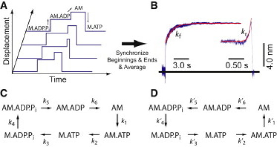
(A) Schematic displacement traces showing the two-step nature of actomyosin interactions in the optical trap. Biochemical intermediates are correlated with displacement states. (B) Ensemble-averaged interactions acquired at 25 μM MgATP (n = 805). Single attachments were synchronized at the times when the attachments start (left) or end (right). (Red lines) Fits of the averages to single exponential rate functions (k_f = 0.77 s⁻¹; k_r = 14 s⁻¹). (C) Forward and (D) time-reversed schemes for actomyosin attachment events.

Figure 2.

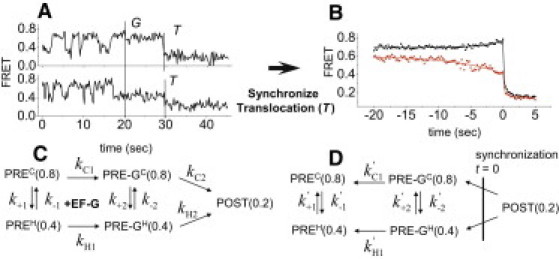
smFRET traces and reaction schemes for EF-G promoted translocation. (A) The smFRET recordings show transitions between PRE^C and PRE^H before EF-G injection (G) and translocation to POST (T) after EF-G injection. (B) Post-synchronized, averaged translocation traces of fluctuating complexes translocated from PRE^C (black) or PRE^H (red). (C) Forward and (D) time-reversed schemes of translocation. Numbers in parentheses are FRET values.

For traces that are synchronized on attachment, the forward time constant (τ_f) between attachment (producing 5.1-nm displacement) and the 8.4-nm state is the lifetime of AM·ADP state (Fig. 1 A). Thus, the rate constant (k_f = 1/τ_f) corresponds to ADP release (k₆), which, at low forces, matches the ADP release rate found in ensemble stop-flow experiments on suspensions of actomyosin.

For the traces that are synchronized on detachment, the reaction step that determines the lifetime of AM and thus the rate of the displacement increase (k_r) before detachment, is ATP binding (k₁; Fig. 1 C). Note the rising phase of the traces preceding detachment have the form of exp(+k_rt) (Fig. 1 B). The positive exponent, unusual in the biological context, arises from the decay extending backward in time.

To determine the origin of k_r by a route that can be applied to more complicated schemes, the procedure outlined above is followed: Step 1. Not necessary, as Fig. 1 C is a complete cycle. Step 2. P(A) = [AM·ADP] = 1/(k₆Σ) and P(B) = [AM] = 1/(k₁Σ), where Σ = Σ_j (1/k_j). Step 3. Applying Eq. 3, k′₆ (in Fig. 1 D) = [1/(k₆Σ)] k₆ / [1/(k₁Σ)] = k₁. Step 4. The measured rate constant leading up to the detachment trigger, k_r = k′₆, is shown to equal k₁, as expected. This simple example was originally analyzed (6) without considering the Bayes' theorem, because the reaction is not branched and in the experiment, the P_i and ADP release steps are irreversible. Further relationships between the two schemes, e.g., k′₁ = k₂, k′₂ = k₃, k′₃ = k₄, etc., also apply.

Another example, less obvious due to reverse reactions and branching, is elongation factor (EF)-G catalyzed translocation of mRNA and tRNAs on the ribosome during protein synthesis (8). Before translocation, tRNAs in the ribosome adopt two interconverting pretranslocation (PRE) conformations, named “classical” and “hybrid” states (PRE^C and PRE^H in Fig. 2) (12). EF-G·GTP promotes translocation of the mRNA and tRNAs from both PRE states to the posttranslocation state (POST). Transitions between PRE^C and PRE^H states before EF-G injection and translocation from PRE states to the POST state after EF-G injection are detected by changes of FRET signals from Cy3-Cy5 FRET pairs positioned on ribosomal large subunit protein L11, near the amino-acyl tRNA entrance site (the A-site), and tRNA in the A-site (Fig. 2 A) (8). Addition of EF-G decreases fluctuations between PRE-G^C and PRE-G^H states before translocation, which is apparent in the recordings of Fig. 2 A that have long dwell times between EF-G injection and translocation (reactions k_C2 and k_H2). In traces from the same population with less time between EF-G binding and translocation, the decrease of classic-hybrid fluctuations is less obvious without detailed analysis.

Single molecule translocation traces were classified into two groups based on the last state (PRE^C or PRE^H) before translocation and post-synchronized using the large decrease of FRET upon translocation as the trigger (Fig. 2 B). The time courses of the averaged traces preceding the trigger event are of interest here. They contain information on the transition rates (k₊₂ and k₋₂, Fig. 2 C) between the two PRE-states after EF-G binding. The rate constants for the synchronized traces leading up to the trigger are much slower than (k₊₁ + k₋₁), suggesting that k₊₂ and k₋₂ are much smaller. To quantify how much smaller requires analysis of the full scheme.

The translocation scheme (Fig. 2 C) (8) does not have a nonzero steady-state solution, because it does not form a complete cycle. Therefore, we introduced an extra reaction from the last state (POST) to the first state (the mixture of PRE^C and PRE^H at equilibrium) to form a complete cycle. Through the stepwise procedure described above, we deduced algebraic expressions for transition rates of the requisite time-reversed scheme (Fig. 2 D). The time-reversed rates, which are essential for characterizing the time course leading up to the trigger in the post-synchronized traces, are independent of the rate constants of the introduced cycle-completion reaction. After applying reaction rates obtained from experimental measurements (8,13) and exponential fitting of the synchronized curves (Fig. 2 B), the transition rates between the two PRE-G states (k₊₂ and k₋₂) were found to be 5–60-fold slower than the transition rates between the two PRE states (k₊₁ and k₋₁) (see details in the Supporting Material). Small values of k₊₂ and k₋₂ are consistent with our observation that ∼5% traces showed classic ↔ hybrid transitions between EF-G injection and translocation. Thus, EF-G binding suppresses transitions between the classical and hybrid PRE states before translocation. This finding is consistent with our earlier report that was originally deduced through a laborious qualitative method (8).

The events after a synchronized trigger step can be interpreted straightforwardly. The events leading up to a trigger point are determined by the lifetimes of the preceding states and the reaction step that produces the trigger event. However, reverse reactions and branches in the scheme make this concept more complicated. Here we described a procedure for dealing with these situations.