Suppressing cascades of load in interdependent networks

Abstract

Understanding how interdependence among systems affects cascading behaviors is increasingly important across many fields of science and engineering. Inspired by cascades of load shedding in coupled electric grids and other infrastructure, we study the Bak–Tang–Wiesenfeld sandpile model on modular random graphs and on graphs based on actual, interdependent power grids. Starting from two isolated networks, adding some connectivity between them is beneficial, for it suppresses the largest cascades in each system. Too much interconnectivity, however, becomes detrimental for two reasons. First, interconnections open pathways for neighboring networks to inflict large cascades. Second, as in real infrastructure, new interconnections increase capacity and total possible load, which fuels even larger cascades. Using a multitype branching process and simulations we show these effects and estimate the optimal level of interconnectivity that balances their trade-offs. Such equilibria could allow, for example, power grid owners to minimize the largest cascades in their grid. We also show that asymmetric capacity among interdependent networks affects the optimal connectivity that each prefers and may lead to an arms race for greater capacity. Our multitype branching process framework provides building blocks for better prediction of cascading processes on modular random graphs and on multitype networks in general.

Networks that constitute our critical infrastructure increasingly depend on one another, which enables cascades of load, stress, and failures (1–6). The water network, for instance, turns turbines and cools nuclear reactors in the electrical grid, which powers the transportation and communications networks that underpin increasingly interdependent global economies. Barrages of disturbances at different scales—volcanic eruptions (7), satellite malfunctions (4), earthquakes, tsunamis, wars (8)—trigger cascades of load shedding in interdependent transportation, communication, and financial systems. Interdependence can also increase within a particular infrastructure, with consequences for cascading failures. The electrical grid of the United States, for example, consists of over 3,200 independent grids with distinct ownership—some private, others public—and unique patterns of connectivity, capacities, and redundancies (9). To accommodate rising demand for electricity, long-distance trade of energy (10), and new types of power sources (11), interconnections among grids bear ever more load (12), and many new high-capacity transmission lines are planned to interconnect grids in the United States and in Europe (13). Fig. 1 shows the interconnections planned to transport wind power (11). Though necessary, these interconnections affect systemic risk in ways not well understood, such as in the power grid, where the modular structure affects its large cascades. For example, the August 14, 2003 blackout, the largest in North American history, spread from a grid in Ohio to one in Michigan, then to grids in Ontario and New York before overwhelming the northeast (10, 14).

Fig. 1.

The power grid of the continental United States, illustrating the three main regions or “interconnects”—Western, Eastern, and Texas—and new lines (in red) proposed by American Electric Power to transport wind power (11, 13).

Researchers have begun to model cascades of load and failure within individual power grids using probabilistic models (15), linearized electric power dynamics (16, 17), and game theory (18). The first models of interdependent grids use simplified topologies and global coupling to find that interconnections affect critical points of cascades (19), which suggests that they may affect the power law distributions of blackout size (12, 15). Models with interconnections among distinct infrastructure have focused on the spread of topological failures, in which nodes are recursively removed (20–22), and not on the dynamical processes occurring on these networks. These models find that interdependence causes alarmingly catastrophic cascades of failed connectivity (20–22). Yet as we show here, interdependence also provides benefits, and these benefits can balance the dangers at stable critical points.

Here we develop a simple, dynamical model of load shedding on sparsely interconnected networks. We study Bak–Tang–Wiesenfeld sandpile dynamics (23, 24) on networks derived from real, interdependent power grids and on sparsely coupled, random regular graphs that approximate the real topologies. Sandpile dynamics are paradigms for the cascades of load, self-organized criticality, and power law distributions of event sizes that pervade disciplines, from neuronal avalanches (25–27) to cascades among banks (28) to earthquakes (29), landslides (30), forest fires (31, 32), solar flares (33, 34), and electrical blackouts (15). Sandpile cascades have been extensively studied on isolated networks (35–41). On interdependent (or modular) networks, more basic dynamical processes have been studied (42–45), but sandpile dynamics have not.

We use a multitype branching process approximation and simulations to derive at a heuristic level how interdependence affects cascades of load. Isolated networks can mitigate their largest cascades by building interconnections to other networks, because those networks provide reservoirs to absorb excess load. Build too many interconnections, however, and the largest cascades in an individual network increase in frequency for two reasons: Neighboring networks inflict load more easily, and each added interconnection augments the system’s overall capacity and load. These stabilizing and destabilizing effects balance at a critical amount of interconnectivity, which we analyze for synthetic networks that approximate interdependent power grids. As a result of the additional load introduced by interconnections, the collection of networks, viewed as one system, suffers larger global cascades—a warning for the increasing interdependence among electrical grids (Fig. 1), financial sectors, and other infrastructure (11–13). Finally, we study the effects of capacity and load imbalance. Networks with larger total capacity inflict larger avalanches on smaller capacity networks, which suggests an arms race for greater capacity. The techniques developed here advance the theoretical machinery for dynamical processes on multitype networks as well as our heuristic understanding of how interdependence and incentives affect large cascades of load in infrastructure.

Theoretical Formulation

Sandpile Dynamics.

Introduced by Bak, et al. in 1987 and 1988 (23, 24), the sandpile model is a well-studied, stylized model of cascades that exhibits self-organized criticality, power laws, and universality classes, which has spawned numerous related models with applications in many disciplines (e.g., refs. 30, 31, 33, 34, and 46). In a basic formulation on an arbitrary graph of nodes and edges, one drops grains of sand (or “load”) uniformly at random on the nodes, each of which has an innate threshold (or capacity). Whenever the load on a node exceeds its threshold, that node topples, meaning that it sheds (or moves) its sand to its neighbors. These neighbors may in turn become unstable and topple, which causes some of their neighbors to topple, and so on. In this way, dropping a grain of sand on the network can cause a cascade of load throughout the system—often small but occasionally large. The cascade finishes once no node’s load exceeds its capacity, whereupon another grain of sand is dropped, and the process repeats. Probability measures of the size, area, and duration of avalanches typically follow power laws asymptotically in the limit of many avalanches (47).

Many classic versions of the sandpile model (23, 46, 47) connect the nodes in a finite, two-dimensional lattice and assign all nodes threshold four, so that a toppled node sheds one sand grain to each of its four neighbors. The lattice has open boundaries, so that sand shed off the boundary is lost, which prevents inundation of sand. A few variants of the model on lattices can be solved exactly if the shedding rules have Abelian symmetry (47).

More recently, sandpile models have been studied on isolated networks, including Erdős-Rényi graphs (35, 36), scale-free graphs (39–41), and graphs generated by the Watts–Strogatz model on one- (37) and two-dimensional (38) lattices. A natural choice for the capacities of nodes—which we use here—is their degree, so that toppled nodes shed one grain to each neighbor (39, 48). Other choices include identical (39), uniformly distributed from zero to the degree k (40), and k^1-η for some 0 ≤ η < 1 (40, 41), but all such variants must choose ways to randomly shed to a fraction of neighbors. Shedding one grain to each neighbor is simpler and exhibits the richest behavior (39). A natural analog of open boundaries on finite lattices is to delete grains of sand independently with a small probability f as they are shed. We choose the dissipation rate of sand f so that the largest cascades topple almost the entire network.

The mean-field solution of sandpile cascades is characterized by an avalanche size distribution that asymptotically obeys a power law with exponent -3/2 and is quite robust to network structure. (For example, on scale-free random graphs, sandpile cascades deviate from mean-field behavior only if the degree distribution has a sufficiently heavy tail, with power law exponent 2 < γ < 3; ref. 39.) Nevertheless, sparse connections among interdependent networks divert and direct sandpile cascades in interesting, relevant ways.

Topologies of Interacting Networks.

Here we focus on interdependent power grids and idealized models of them. We obtained topological data on two interdependent power grids—which we label c and d—from the US Federal Energy Regulation Commission (FERC).* (All data shown here are sanitized to omit sensitive information.) Owned by different utilities but connected to one another in the southeastern United States,^† power grids c and d have similar size (439 and 504 buses) but rather different average internal degrees (2.40 and 2.91, respectively). The grids are sparsely interconnected by just eight edges, making the average external node degrees 0.021 and 0.018, respectively. More information on c and d is in Table S1. As in other studies, we find that these grids have narrow degree distributions (49–51) and are sparsely interconnected to one another (12).

To construct idealized versions of the real grids, consider two networks labeled a and b. Because of the narrow degree distribution of the real grids, we let network a be a random z_a-regular graph (where each node has degree z_a) and network b be a random z_b-regular graph. These two are then sparsely interconnected as defined below. To define this system of coupled networks more formally, we adopt the multitype network formalism of refs. 45 and 52. Each network a, b has its own degree distribution, p_a(k_aa,k_ab) and p_b(k_ba,k_bb), where, for example, p_a(k_aa,k_ab) is the fraction of nodes in network a with k_aa neighbors in a and k_ab in b. We generate realizations of multitype networks with these degree distributions using a simple generalization of the configuration model: All nodes repeatedly and synchronously draw degree vectors (k_oa,k_ob) from their degree distribution p_o (where o∈{a,b}), until the totals of the internal degrees k_aa, k_bb are both even numbers and the totals of the external degrees k_ab, k_ba are equal.^‡

We interconnect the random z_a, z_b-regular graphs by Bernoulli-distributed coupling: each node receives one external “edge stub” with probability p and none with probability 1 - p. Hence the degree distributions are p_a(z_a,1) = p, p_a(z_a,0) = 1 - p, and p_b(1,z_b) = p, p_b(0,z_b) = 1 - p. We denote this class of interacting networks by the shorthand R(z_a)-B(p)-R(z_b); we illustrate a small example of R(3)-B(0.1)-R(4) in Fig. 2.

Fig. 2.

A random three- and four-regular graph connected by Bernoulli-distributed coupling with interconnectivity parameter p = 0.1 [R(3)-B(0.1)-R(4)]. We also illustrate the shedding branch distribution q_ab(r_ba,bb), the chance that an ab shedding causes r_ba, r_bb many ba, bb sheddings at the next time step. Note these random graphs are small and become tree-like when they are large (⪆1,000 nodes).

Measures of Avalanche Size.

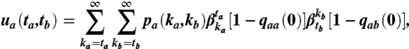
We are most interested in the avalanche size distributions s_a(t_a,t_b),s_b(t_a,t_b), where, for example, s_a(t_a,t_b) is the chance that an avalanche begun in network a (indicated by the subscript on s_a) causes t_a, t_b many topplings in networks a, b, respectively. These distributions count the first toppling event, and they are defined asymptotically in that s_a, s_b are frequencies of avalanche sizes after the networks have undergone many cascades. To study s_a and s_b, we simulate sandpile avalanches and approximate them using a multitype branching process.

Multitype Branching Process Approximation.

In these next two sections, we present an overview of our mathematical formulation, with details left to Materials and Methods. We develop a branching process approximation that elucidates how sandpile cascades spread in interconnected networks, advances theoretical tools for cascades on multitype networks, justifies using this model as an idealization of real infrastructure like power grids, and establishes an open and relevant mathematical challenge. However, readers more interested in the applications of the model may wish to skip to Results.

Sandpile cascades on networks can be approximated by a branching process provided that the network is locally tree-like (i.e., has few short cycles), so that branches of a nascent cascade grow approximately independently. The interacting networks R(z_a)-B(p)-R(z_b) are tree-like provided they are sparse and large enough (with at least several hundred nodes) because the edges are wired uniformly at random. Power grids are approximately tree-like: The clustering coefficient of power grids c and d, for example, is C ≈ 0.05, an order of magnitude larger than an Erdős-Rényi random graph with equally many nodes and edges, but still quite small. Although tree-based approximations of other dynamical processes work surprisingly well even on non-tree-like graphs, power grid topologies were found to be among the most difficult to predict with tree-based theories (54). Here we find that analytic, tree-based approximations of sandpile dynamics agree well with simulations even on the real power grid topologies (Fig. 3 and Figs. S1 and S2).

Fig. 3.

The multitype branching process (red curves) approximates simulations of sandpile cascades on the power grids c, d (blue curves) surprisingly well, given that power grids are among the most difficult network topologies on which to predict other dynamics (54). We plot the four marginalized avalanche size distributions (using the labels a, b for grids c, d). For example, Fig. 3A, plotting versus t_a, is the chance an avalanche begun in a topples t_a nodes in a. Vertical axes’ labels are the expressions in the plots. Here dissipation f = 0.1.

Cascades on interacting networks require a multitype branching process, in which a tree grows according to probability distributions of the number of events of various types generated from seed events. We consider two basic event types, a and b topplings—i.e., toppling events in networks a and in b. These simplify the underlying branching process of sheddings, or grains of sand shed from one network to another, of which there are four types: aa, ab, ba, and bb sheddings. (Note that there is no distinction between topplings and sheddings on one, isolated network, because sand can only be shed from, say, a to a.)

A key property of sandpile dynamics on networks, which enables the branching process calculations, is that in simulations the amount of sand on a node is asymptotically uniformly distributed from zero to one less its degree (i.e., there is no typical amount of sand on a node) (48, 55). Hence the chance that a grain arriving at a node with degree k topples it equals the chance that the node had k - 1 grains of sand, which is 1/k. So sandpile cascades are approximated by what we call 1/k percolation: The cascade spreads from node u to node v with probability inversely proportional to the degree of v. That this probability decays inversely with degree suggests a direct interpretation for infrastructure: Important nodes have k times more connectivity than unimportant (degree 1) nodes, so they are k times less likely to fail (they are presumably reinforced by engineers). But when important nodes do fail, they cause k times more repercussions (shedded grains of sand). We found some evidence for this inverse dependence on degree in the power flowing through buses (nodes) in power grids: Each additional degree correlates with an additional 124 mVA of apparent power flowing through it (R² = 0.30; see Fig. S3).

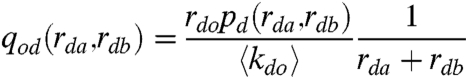
The details of the branching process analysis extend the standard techniques as presented in Materials and Methods. We give here only the crux of the derivation. Suppose a grain of sand is shed from network o∈{a,b} to network d∈{a,b} (origin network, o; destination network, d). What is the chance that this grain shed from o to d (an od shedding) causes r_da and r_db many grains to be shed from network d to a and from d to b, respectively, at the next time step? This probability distribution, denoted q_od(r_da,r_db), is the branch (or children) distribution of the branching process for sheddings. Fig. 2 illustrates q_ab as an example. Neglecting degree–degree correlations [the subject of so-called P(k,k^′) theory; ref. 54], a grain shed from network o to d arrives at an edge stub chosen uniformly at random, so it arrives at a node with degree p_d(r_da,r_db) with probability proportional to r_do because that node has r_do many edges pointing to network o. Using this fact and the chance of toppling found above (1/total degree), we approximate asymptotically that

[1]

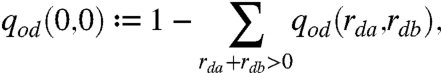
for r_da + r_db > 0, where is the expected number of edges from d to o, . To normalize q_od, set

[2]

which is the probability that the destination node does not topple (i.e., that it has fewer grains than one less its total degree).

Note that for an individual, isolated network the analogous branch distribution q(k) simplifies considerably: In the equivalent of Eq. 1 there is a cancellation of k in the numerator of with 1/k on the right (39–41). Thus the expected number of children events . Each seed event gives rise to one child on average, which then gives rise to one child on average, etc., which is called a “critical” branching process. (If less than one child on average, the branching process dies out; if more than one it may continue indefinitely.) The branching process approximations of sandpile cascades on the interacting networks studied here—coupled random regular graphs a, b and power grids c, d—are also critical, because the principle eigenvalue of the matrix of first moments of the branch distributions is one.

The branching process of sheddings is high dimensional, with four types aa, ab, ba, bb recording origin and destination networks. Transforming the shedding branch distributions q_od to the toppling branch distributions u_a, u_b is easy; the key is that a node topples if and only if it sheds at least one grain of sand (for details, see Materials and Methods). Transforming to toppling distributions also halves the dimensions of the branching process of topplings, simplifying calculations.

Self-Consistency Equations.

We analyze implicit equations for the avalanche size distributions s_a, s_b using generating functions (56). Denote the generating functions associated to the toppling branch distributions u_a, u_b and the avalanche size distributions s_a, s_b by capital letters and ; for example,

The theory of multitype branching processes (57) implies the self-consistency equations

[3]

where each is evaluated at (τ_a,τ_b). In other words, the left-hand equation in [3] says that, to obtain the distribution of the sizes of cascades begun in a, the cascade begins with an a toppling (hence the τ_a out front), which causes at the next time step a number of a and b topplings distributed according to , and these topplings in turn cause numbers of a and b topplings distributed according to and .

We wish to solve Eq. 3 for and , because their coefficients are the avalanche size distributions s_a, s_b of interest. In practice, however, these implicit equations are transcendental and difficult to invert. Instead, we solve Eq. 3 with computer algebra systems using three methods—iteration, Cauchy integral formula, and multidimensional Lagrange inversion (58)—to compute exactly hundreds of coefficients; for details, see Materials and Methods. Fig. 3 shows good agreement between simulation of sandpile cascades on power grids c, d and the branching process approximation (obtained by iterating Eq. 3 seven times starting from , with branch distributions calculated from the empirical degree distributions of c, d). For more details on the agreement, including how the degrees of nodes with external links account for the characteristic “blips” in the avalanche size distributions of the power grids, see Figs. S1 and S2.

These numerical methods are computationally feasible for the probabilities of the smallest avalanches, but we are most interested in the probabilities of the largest avalanches—that is, in the asymptotic behaviors of s_a(t_a,t_b),s_b(t_a,t_b) as t_a,t_b → ∞. Unfortunately the technique used for an isolated network—an expansion at a singularity of —fails for sandpile cascades on Bernoulli-coupled random regular graphs and on the power grids, because their generating functions have singularities at infinity and none in the finite plane (see Materials and Methods). Generalizing these asymptotic techniques to “multitype cascades” with singularities at infinity poses an outstanding mathematical challenge. Nevertheless, three tactics—simulations, computer calculations of coefficients of , , and analytical calculations of the first moments of the branch and avalanche size distributions—suffice to obtain interesting conclusions about the effect of interdependence on critical cascades of load, as discussed next.

Results

Locally Stabilizing Effect of Interconnections.

We first answer this question, would an isolated network suppress its largest cascades of load by connecting to another network? For coupled random regular graphs R(z_a)-B(p)-R(z_b), yes; increasing interconnectivity p suppresses an individual network’s largest cascades, but only up to a critical point p^∗ (Fig. 4).

Fig. 4.

Interconnectivity is locally stabilizing, but only up to a critical point. The main plot, the results of simulations on R(3)-B(p)-R(3) (2 × 10⁶ grains; f = 0.01; 2 × 10³ nodes/network), shows that large local cascades decrease and then increase with p, whereas large inflicted cascades only become more likely. Their average (gold curve) has a stable minimum at p^∗ ≈ 0.075 ± 0.01. This curve and its critical point, p^∗, are stable for cutoffs in the regime . (Insets) Rank-size plots on log–log scales of the largest cascades in network a (Left) for p = 10^-3, 10^-2, 10^-1 and in power grid d connected to c by 0, 8, or 16 edges.

First we introduce notation. For a cascade that begins in network a, the random variables T_aa, T_ab are the sizes of the “local” and “inflicted” cascades: The number of topplings in a and in b, respectively. For example, a cascade that begins in a and that topples 10 a nodes and 5 b nodes corresponds to T_aa = 10, T_ab = 5. We denote T_a to be the random variable for the size of a cascade in network a, without distinguishing where the cascade begins. (We define T_ba, T_bb, T_b analogously.) Dropping sand uniformly at random on two networks of equal size means that avalanches begin with equal probability in either network, so .

In Fig. 4 we plot the probability of observing a large avalanche in a (that topples at least half of all its nodes) as a function of interconnectivity p, as measured in numerical simulations on the R(3)-B(p)-R(3) topology. We distinguish between those avalanches that begin in a (blue local cascades), begin in b (red inflicted cascades), or in either network (gold). With increasing interconnectivity p, large inflicted cascades from b to a (red curve) increase in frequency due in large part to the greater ease of avalanches traversing the interconnections between networks. More interesting is that increasing interconnectivity suppresses large local cascades (blue curve) for small p, but amplifies them for large p. The 80% drop in Pr(T_aa > 1,000) and 70% drop in Pr(T_a > 1,000) from p = 0.001 to p^∗ ≈ 0.075 ± 0.01 are the locally stabilizing effects of coupling networks. The left inset in Fig. 4 is the rank-size plot showing the sizes of the largest avalanches and their decrease with initially increasing p, and the same holds for simulations on the power grids c and d (right inset).^§ The curve and the location of its critical point p^∗ in Fig. 4 is robust to changing the cutoff . Thus a network such as a seeking to minimize its largest cascades would seek interconnectivity that minimizes , which we estimate to be p^∗ ≈ 0.075 ± 0.01 for R(3)-B(p)-R(3) with 2 × 10³ nodes per network.

This central result appears to be generic: changing the system size, internal degrees, or type of degree distribution (so long as it remains narrow) may slightly change p^∗ but not the qualitative shape of Fig. 4 (see Figs. S4 and S5). Furthermore, this effect of optimal connectivity is unique to interconnected networks: adding edges to a single, isolated network does not reduce the chance of a large cascade (and hence produce a minimum like in Fig. 4). [This result for an isolated network is expected because s(t) ∼ t^-3/2 for all narrow degree distributions; ref. 39.] Whereas adding links within a network can only increase its vulnerability to large cascades, adding links to another network can reduce it. Note that we cannot derive analytical results for Fig. 4 because the standard techniques for single networks fail for multitype generating functions with singularities at infinity, and inverting Eq. 3 numerically is practical only for exactly computing the probabilities of small cascades (T_a < 50) and not large ones (T_a > 10³) (see Materials and Methods).

Intuitively, adding connections between networks diverts load, and that diverted load tends to be absorbed by the neighboring network rather than amplified and returned, because most cascades in isolated networks are small. One way to see the diversion of load is in the first moments of the toppling branch distributions u_a, u_b. For R(z_a)-B(p)-R(z_b), the average numbers of topplings at the next time step in the same and neighboring networks, respectively, decrease and increase with the interconnectivity p as , where, for example, .

However, introducing too many interconnections is detrimental, as shown in Fig. 4. Interconnections let diverted load more easily return and with catastrophic effect. In addition, each interconnection augments the networks’ capacity and hence average load, so that large avalanches increase in frequency in individual networks and in the collection of networks, as discussed next.

Globally Destabilizing Effect of Interconnections.

Adding interconnections amplifies large global cascades. That is, the largest avalanches in the collection of networks—viewed as one system with just one type of node—increase in size with interconnectivity. Here we are interested in the total avalanche size distribution s(t), the chance of t topplings overall in a cascade. Fig. 5 shows the extension of the right-hand tail of s(t) in simulations on R(3)-B(p)-R(3) with increasing interconnectivity p. The rank-size plot inset shows more explicitly that the largest avalanches increase with p. Similar results occur in simulations on power grids c, d (see SI Text).

Fig. 5.

Increasing the interconnectivity p between two random three-regular graphs extends the tail of the total avalanche size distribution s(t), which does not distinguish whether toppled nodes are in network a or b. The inset shows a rank-size plot on log–log scales of the number of topplings t in the largest 10⁴ avalanches (with 2 × 10⁶ grains of sand dropped), showing that adding more edges between random three-regular graphs enlarges the largest global cascades by an amount on the order of the additional number of interconnections. As expected theoretically (39), when a and b nodes are viewed as one network, s(t) ∼ t^-3/2 for large t (green line).

What amplifies the global cascades most significantly is the increase in total capacity (and hence average load available for cascades) and not the increased interdependence between the networks. (Recall that capacities of nodes are their degrees, so introducing new edges between networks increments those nodes’ degrees and capacities.) To see this effect on coupled random regular graphs, we perform the following rewiring experiment. Beginning with two isolated random regular graphs, each node changes one of its internal edge stubs to be external with probability p. The degree distributions become, for example, p_a(z_a - 1,1) = p, p_a(z_a,0) = 1 - p, which we call “correlated-Bernoulli coupling” because the internal and external degrees are not independent. Fig. S6 shows that the largest global avalanches are not significantly enlarged with increasing “rewired interconnectivity” p for random three-regular graphs with such coupling. Furthermore, the enlargement of the largest cascades observed in the rank-size plot in the inset of Fig. 5 is on the order of the extra average load resulting from the additional interconnectivity (and the same holds for simulations on the power grids).

The amplification of global avalanches, though relatively small, is relevant for infrastructure: Additional capacity and demand often accompany—and even motivate—the construction of additional interconnections (11, 13). Furthermore, in reality it is more common to augment old infrastructure with new interconnections as in Fig. 1 (Bernoulli coupling) rather than to delete an existing internal connection and rewire it to span across networks (correlated-Bernoulli coupling). Thus, building new interconnections augments the entire system’s capacity, and hence average load, and hence largest cascades.

Interconnectivity That Mitigates Cascades of Different Sizes.

Fig. 4 shows that networks seeking to mitigate their large avalanches seek optimal interconnectivity p. Networks mitigating their small or intermediate cascades would seek different optimal interconnectivity p, as shown in Fig. 6 [the results of simulations on R(3)-B(p)-R(3)]. Fig. 6A shows that the probability of a small cascade in network a (1 ≤ T_a ≤ 51) increases monotonically with p, so that networks mitigating the smallest cascades seek isolation, p = 0. By contrast, the chance of a cascade of intermediate size, 100 ≤ T_a ≤ 150 (Fig. 6B), has a local maximum at p^∗ ≈ 0.05, so networks mitigating intermediate cascades would demolish all interconnections (p = 0) or build as many as possible (p = 1). By contrast, the largest cascades 400 ≤ T_a ≤ 1,500 (Fig. 6 C and D) occur with minimal probability at p^∗ ≈ 0.075 ± 0.01. For more plots showing the change in concavity and the robustness of the stable critical point p^∗ for large cascades, see Fig. S7.

Fig. 6.

(A) Networks mitigating the smallest cascades 1 ≤ T_a ≤ 51 seek isolation p = 0, whereas (B) networks suppressing intermediate cascades 100 ≤ T_a ≤ 150 seek isolation p = 0 or strong coupling p = 1, depending on the initial interconnectivity p in relation to the unstable critical point p^∗ ≈ 0.05. But networks like power grids mitigating large cascades (C and D) would seek interconnectivity at the stable equilibrium p^∗ ≈ 0.075 ± 0.01. The bottom figures and the location of p^∗ are robust to changes in the window ℓ ≤ T_a ≤ ℓ + 50 for all 400 ≤ ℓ ≤ 1,500.

Other models of cascades in power grids conclude that upgrading and repairing the system to mitigate the smallest blackouts may increase the risk of the largest blackouts (15). Similarly, extinguishing small forest fires, a common policy in the 20th century, increases forest vegetation and thus the risk of large forest fires—a phenomenon known as the “Yellowstone effect” (32). The results here augment these conclusions to include interconnectivity. Networks building interconnections in order to suppress their large cascades cause larger global cascades (by an amount on the order of the additional capacity). Networks suppressing their small or intermediate cascades may seek isolation (p = 0), which amplifies their large cascades, or (for intermediate cascades) strong coupling (p = 1), which amplifies both large local and global cascades.

Capacity Disparity.

Two networks that are interdependent are rarely identical, unlike the R(3)-B(p)-R(3) topologies studied thus far, so we determine the effect of capacity disparity on cascades. Because the capacities of nodes are their degrees, we study R(z_a)-B(p)-R(z_b) with different internal degrees, z_a ≠ z_b. We find that interdependence is more catastrophic for smaller capacity networks, in that they suffer comparatively larger inflicted cascades. They still prefer some interconnectivity, but less than the higher capacity network.

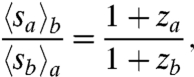
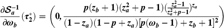
Using the theoretical branching process approximation, we compute how much larger inflicted cascades are from high- to low-capacity networks. Differentiating Eq. 3 with respect to τ_a, τ_b and setting τ_a = τ_b = 1 yields four linear equations for the first moments of the avalanche size distributions s_a, s_b in terms of the first moments of the branch distributions u_a, u_b. For R(z_a)-B(p)-R(z_b), the four first moments of s_a, s_b are all infinite, as expected, because in isolation these networks’ avalanche size distributions are power laws with exponent -3/2 (39–41). Nevertheless, we can compare the rates at which the average inflicted cascade sizes diverge by computing their ratio

[4]

where, e.g., (see SI Text for the derivation). Thus z_b > z_a implies that the inflicted cascades from b to a are larger on average than those from a to b. Fig. S8 shows qualitative agreement with simulations.

As a result of Eq. 4, the low-capacity network prefers less interconnectivity than the high-capacity network. In simulations of R(3)-B(p)-R(4), for instance, low-capacity network a prefers , whereas high-capacity b prefers . For systems like power grids seeking to mitigate their cascades of load, these results suggest an arms race for greater capacity to fortify against cascades inflicted by neighboring networks.

Incentives and Equilibria in Power Grids.

Because different networks have unique susceptibilities to cascades (due to capacity disparity, for example), equilibria among real networks are more nuanced than on identical random graphs. Next we explore how the level of interconnectivity and load disparity affect sandpile cascades on the power grids c and d. [Although sandpile dynamics do not obey Ohm’s and Kirchoff’s laws nor the flow of load from sources to sinks, as in physical power flow models (e.g., refs. 16 and 17), they do closely resemble some engineers’ models of blackouts, and blackout data show evidence of criticality and power laws; ref. 15.] To interpret results, we suppose that the owners of the power grids c, d are rational, in that they wish to mitigate their largest cascades but care little about cascades overwhelming neighboring grids.

To capture different amounts of demand, numbers of redundancies, ages of infrastructure, susceptibility to sagging power lines (16, 17), and other factors that affect the rate at which cascades of load shedding and failures begin in each network, we introduce a load disparity parameter r as follows. Each node in c is r times more likely than a node in d to receive a new grain of sand. Increasing r intensifies the load on grid c, the rate at which cascades begin there, and the sizes of the largest inflicted cascades from c to d. The larger r is, the more volatile power grid c becomes.

Given the spatial structure of the power grid networks, there is no principled way to add arbitrarily many interconnections between them. However, three different levels of interconnectivity are natural: (i) Delete the eight interconnections so that c and d are isolated, (ii) leave the eight original interconnections, and (iii) add eight additional interconnections in a way that mirrors the empirical degree distribution.

Fig. 7 shows that there are two ways to amplify the largest inflicted cascades in d. The first is to increase the number of interconnections (compare red to green-dashed curve in the main figure). The second is to increase r (compare distance from green to gold curve in the main figure and in the inset). At a critical r^∗, the largest inflicted cascades in d that begin in c (red and green-dashed curves) are equally large as the largest local cascades in d that begin in d (blue and gold curves). For 16 interconnections, we estimate r^∗ ≈ 15 (Fig. 7, Inset), and the inflicted cascades are larger and smaller, respectively, for r = 10, 20 (Fig. S9)—indicating that inflicted cascades begin to dominate local cascades at r^∗ ≈ 15. The actual load disparity between power grids c and d is r ≈ 0.7, which we estimate by computing the average power incident per node in simulation output from FERC.^§ (There are, however, interdependent power grids in the southeastern United States with r > 15.) Because r = 0.7, the load is greater on grid d, so grid d prefers more interconnections and c prefers fewer than if r were one. Consequently, any equilibrium between the two grids is frustrated (or semistable): Only one grid can achieve its desired interconnectivity.

Fig. 7.

The critical load disparity at which inflicted cascades in d become equally large as its local cascades is r^∗ ≈ 15 (for 16 interconnections, “bridges”). (For eight interconnections, r^∗ > 20; see Fig. S9). Here we show a rank-size plot in log–log scales of the largest 10⁴ avalanches in power grid d, distinguishing whether they begin in c (inflicted cascades) or in d (local cascades), for 8 and 16 interconnections (solid, dashed curves), for r = 1 (Main), r = 15 (Inset), in simulations with dissipation of sand f = 0.05, 10⁶ grains dropped after 10⁵ transients.

Discussion

We have presented a comprehensive study of sandpile cascades on interacting networks to obtain a deeper understanding of cascades of load on interdependent systems, showing both the benefits and dangers of interdependence. We combine a mathematical framework for multitype networks (45, 52) with models of sandpiles on isolated networks (35–41) to derive a multitype branching process approximation of cascades of load between simple interacting networks and between real power grids. We show that some interdependence is beneficial to a network, for it mitigates its largest avalanches by diverting load to neighboring networks. But too much interconnectivity opens new avenues for inflicted load; in addition, each new interconnection adds capacity that fuels even larger cascades. The benefits and detriments in mitigating large avalanches balance at a critical amount of interconnectivity, which is a stable equilibrium for coupled networks with similar capacities. For coupled networks with asymmetric capacity, the equilibria will be frustrated, in that the networks prefer different optimal levels of interconnectivity.

We also show that tuning interconnectivity to suppress cascades of a certain range of sizes amplifies the occurrence of cascades in other ranges. Thus a network mitigating its small avalanches amplifies its large ones (Figs. 4 and 6), and networks suppressing their own large avalanches amplify large ones in the whole system (Fig. 5). Similarly it has been found that mitigating small electrical blackouts and small forest fires appears to increase the risk of large ones (15, 32). Furthermore, the amplification of global cascades due to the increase in capacity (Fig. 5) is a warning for new interconnections among power grids (11, 13) (Fig. 1), financial sectors, and other infrastructure.

These findings suggest economic and game-theoretic implications for infrastructure. (Note that here we consider the strategic interactions of entire networks rather than of individual nodes in one network, which is more standard, e.g., ref. 59.) For example, a power grid owner wishing to mitigate the largest cascades in her grid would desire some interconnections to other grids, but not too many. However, what benefits individual grids can harm society: Grids building interconnections amplify global cascades in the entire system. More detailed models that combine results like these with economic and physical considerations of electrical grids and with costs of building connections may provide more realistic estimates of optimal levels of interconnectivity. Our framework—which models a dynamical process on stable, underlying network topologies—could also be combined with models of topological failure in interdependent networks (20–22). Those studies conclude that systemic risk of connectivity failure increases monotonically with interdependence (“dependency links”). Whether suppressing cascades of load or of connectivity failures is more important might suggest whether to interconnect some (p^∗ > 0) (Fig. 4) or none (p = 0) (20–22), respectively. Our results are consistent with recent work showing that an intermediate amount of connectivity minimizes risk of systemic default in credit networks (60), in contrast to refs.  20, 21 and the more traditional view that risk increases monotonically with connectivity in credit networks (e.g., ref. 61).

This work also advances our mathematical understanding of dynamical processes on multitype networks. Because networks with one type of node and edge are impoverished views of reality, researchers have begun to study dynamical processes on multitype networks, such as on modular graphs (42–45). Here we derive a branching process approximation of sandpile cascades on multitype networks starting from the degree distributions, and we discuss open problems in solving for the asymptotic behavior of the generating functions’ coefficients, which elude current techniques for isolated networks. We expect that the computational techniques used here to solve multidimensional generating function equations, such as multidimensional Lagrange inversion (58), will find other uses in percolation and cascades in multitype networks. Finally, in the Appendix we derive the effective degree distributions in multitype networks, which expands the admissible degree distributions that others have considered. The machinery we develop considers just two interacting networks, a and b, or equivalently one network with two types of nodes. However, this machinery extends to finitely many types, which may be useful for distinguishing types of nodes—such as buses, transformers, and generators in electrical grids—or for capturing geographic information in a low-dimensional way without storing explicit locations—such as buses in the interiors of power grids and along boundaries between them.

Here we have focused on mitigating large avalanches in modular networks, but other applications may prefer to amplify large cascades, such as the adoption of products in modular social networks (62) or propagating response-driven surveys across bottlenecks between social groups (63). Cascades in social networks like these may require networks with triangles or other subgraphs added (53, 64, 65); inverting the resulting multidimensional generating function equations for dynamics on these networks would require similar multitype techniques as developed here.

We expect that this work will stimulate calculations of critical points in interconnectivity among networks subjected to other dynamics, such as linearized power flow equations in electrical grids (16, 17) and other domain-specific models. As critical infrastructures such as power grids, transportation, communication, banks, and markets become increasingly interdependent, resolving the risks of large cascades and the incentives that shape them becomes ever more important.

Materials and Methods

Power Grid Topologies.

To understand coupling between multiple grids, we requested data from the US Federal Energy Regulation Commission.^§ Using output of power simulations on many connected areas (distinct grids owned by different utilities) in the southeastern United States, we chose grid d by selecting the grid with the highest average internal degree and the grid, c, to which it had the most interconnections (eight). Grids c, d have 439 and 504 buses (nodes) and average internal degrees 2.40 and 2.91. For our purposes here, the only important details are the narrow degree distributions, the low clustering coefficients, and the number of interconnections between the grids. Other details about the grids are in the SI Text.

Toppling Branch Distributions.

To reduce the number of types in the branching process, we count the number of toppling events in each network rather than the number of grains of sand shed from one network to another. Here we derive the toppling branch distributions u_a, u_b from the shedding branch distributions q_od. [For instance, u_a(t_a,t_b) is the chance that a toppled node in a causes t_a, t_b many nodes in a, b to topple at the next time step.] Note that a node topples if and only if it sheds at least one grain of sand. Thus a grain traveling from a network o to network d topples its destination node with probability 1 - q_od(0,0). Denoting (0,0) by 0 and the binomial distribution by , we have

because the node must have at least t_a many a neighbors and at least t_b many b neighbors, only t_a, t_b of which topple (which are binomially distributed). The expression for u_b is analogous. As an example, the probability generating function of u_a for Bernoulli-coupled random regular graphs R(z_a)-B(p)-R(z_b) is

Three Methods for Numerically Solving the Multidimensional Self-Consistency Equations of a Multitype Branching Process.

The most naïve method to solve the self-consistency equations of a multitype branching process (such as Eq. 3) is to use a computer algebra system like Mathematica or Maple to iterate [3] symbolically starting from , expand the result, and collect coefficients. To obtain the coefficient s_a(t_a,t_b) exactly, it suffices to iterate [3] at least t_a + t_b + 1 times. What is more, just a handful of iterations partially computes the tails (coefficients of terms with high powers in , ), but the amount of missing probability mass in the tails is undetermined. This method was used in Fig. 3.

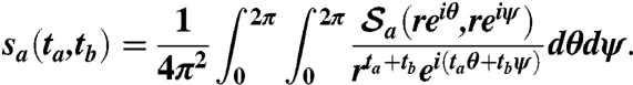
A second method is to symbolically iterate Eq. 3 at least t_a + t_b + 1 times and to use Cauchy’s integral formula

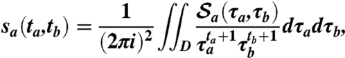[5]

where is a Cartesian product of circular contours centered at the origin, each of radius r smaller than the modulus of the pole of closest to the origin (58). Then calculate one coefficient at a time using

A third method is Lagrange inversion, generalized to multiple dimensions by Good in 1960 (58), a result that has seen little use in the networks literature. We state the theorem in the language of the two-type branching process considered here, with the notation , , and 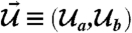. For the slightly more general result that holds for arbitrary, finite, initial population, see ref. 58.

Theorem 1.

[Good 1960] If and (i.e., every type has a positive probability of being barren), then for x∈{0,1},

[6]

where μ, ν run over the types {a,b}, is the Kronecker delta, and ||·|| is the determinant.

Taking x = 0 gives , whereas taking x = 1 gives . In practice, hundreds of terms of , can be computed exactly by truncating the sum in [6] and using computer algebra systems (see Fig. S10 for more details).

Solving for the Coefficients Asymptotically (and Why Standard Techniques Fail).

To determine the asymptotic behaviors of s_a(t_a,t_b), s_b(t_a,t_b) as t_a,t_b → ∞, the trick is to solve for the inverses of and and to expand those inverses and at the singularities of and . This technique works for isolated networks (39–41, 66), but and have no finite singularities in for Bernoulli-coupled random regular graphs nor for power grids c, d.

We demonstrate this failure of standard asymptotic techniques on the networks R(z_a)-B(p)-R(z_b). Let . Assuming an inverse of exists, using [3] we have

[7]

The generating functions , have singularities at , , respectively, if , where the operator is a vector of partial derivatives. Differentiating Eq. 7 and equating the numerators to zero gives

[8a]

[8b]

The only solution to Eq. 8 is

[9a]

[9b]

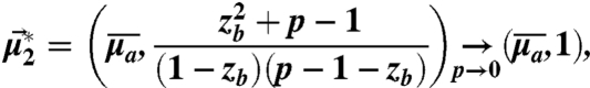
This solution [9] does not recover the singularities (where c₁, c₂ are arbitrary) that we should obtain when the networks are isolated (p = 0) (39). Moreover, although Eqs. 8 vanish at the solutions [9], the derivatives of [7] do not vanish at these solutions [9], because , . Thus we must discard solutions [9].

Solving only the left-hand equations in [8] yields singularities that do recover the correct singularities when p = 0:

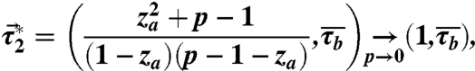[10a]

[10b]

where , are arbitrary constants satisfying

[11]

so that the derivatives of [8] evaluated at [10] are finite. However, the derivatives on the right-hand sides of Eq. 8 (evaluated at the solutions [10]) are

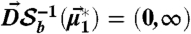
and similarly for (interchange a and b). This derivative vanishes if and only if p = 0 or z_a = 1 or ω_b = ∞. Hence we cannot find finite singularities of , ; these generating functions are entire functions with singularities only at τ_b = μ_a = ∞, , . Hence we have no singularities at which to do an asymptotic expansion for the coefficients s_a, s_b, as one can for isolated networks (39–41, 66).

Other techniques exist for asymptotically approximating the coefficients of generating functions, depending on the type of the singularity (ref. 56, sect. 5). Hayman’s method (ref. 56, sect. 5.4) works for generating functions with no singularities in the finite plane (i.e., entire functions), like the , considered here. However, the theorem requires a closed form expression for the generating function, which we cannot obtain from the self-consistency equations for the synthetic and real interacting networks of interest. Developing techniques for asymptotically approximating the coefficients of multidimensional generating functions with singularities at infinity, like those studied here, poses an important challenge for future studies of dynamical processes on multitype networks.

Appendix: Effective Degree Distributions in Multitype Networks

Using the configuration model to generate multitype networks—including bipartite and multipartite graphs, graphs with arbitrary distributions of subgraphs, and the modular graphs considered here—requires matching edge stubs within and among types. For example, for the interacting networks considered here, the number of edge stubs pointing from network a to network b must equal the number from b to a. A standard practice in the literature (45, 53), which is more restrictive than needed, is to require that the averages of the interdegrees over the degree distributions agree (e.g., for two networks a, b of equal size). In fact, most any degree distributions can be used, as long as conditioning on matching edge stubs among the types of nodes leaves some probability. Requiring that the degree distributions satisfy, for example, , merely tips the scales in favor of valid degree sequences.

Here we derive the effective degree distribution in multitype networks generated with the configuration model. The idea is simple: Because nodes draw degrees independently, the probability distribution of the total number of edge stubs from, say, network a to b is given by a convolution of the degree distribution. We state it for the two interacting networks considered here, but it can be easily generalized to, say, role distributions (53), which require matching edge stubs with ratios different from one.

Suppose networks a, b have N_a, N_b many nodes, respectively. Let , be the random variables for the sequences of “interdegrees” k_ab, k_ba of the nodes in networks a, b, respectively, drawn from the input degree distributions p_a(k_aa,k_ab),p_b(k_ba,k_bb). Suppose, for simplicity, that the internal and external degrees are independent [p_a(k_aa,k_ab) = p_aa(k_aa)p_ab(k_ab), p_b(k_ba,k_bb) = p_ba(k_ba)p_bb(k_bb)], although this is not essential. We denote for

Lemma 1.

With the assumptions in the previous paragraph, the effective interdegree distribution for network a is not the input one, , but rather the conditional probability distribution

where are p_ab, p_ba convolved N_a, N_b times, respectively.

Proof:

Using the independence of and , we have

In the numerator, we recognize to be p_ba convolved N_b times, evaluated at . In the denominator, use independence, recognize convolutions, and sum on ℓ≥0.

Lemma 1 shows that the effective interdegree distribution of a is the input degree distribution p_ab reduced by an amount given by a fraction of convolutions. This reduction in probability governs how many invalid degree sequences must be generated before generating a valid one. For systems sizes on the order of 10⁴ nodes, as considered here, generating degree sequences until producing a valid one is quite feasible, as it takes merely seconds. However, for millions of nodes or more, it is better to generate degree sequences , once, and then repeatedly choose a node uniformly at random to redraw its degree from its degree distribution until the degree sequences are valid. However, this method does not escape the effect in Lemma 1, which is often subtle but can be substantial if the supports of the convolutions of the degree distributions have little overlap. The interdegree distributions used here, Bernoulli and correlated-Bernoulli with identical expected total interdegree, have “much overlap,” so the effective interdegree distribution is approximately the input one, and the correction factor in Lemma 1 can be neglected.

References

- 1.Little RG. Controlling cascading failure: Understanding the vulnerabilities of interconnected infrastructures. J Urban Technol. 2002;9:109–123. [Google Scholar]
- 2.Rinaldi SM. Modeling and simulating critical infrastructures and their interdependencies; 38th Hawaii International Conference on System Sciences; Washington, DC: IEEE Computer Society; 2004. pp. 1–8. [Google Scholar]
- 3.Pederson P, Dudenhoeffer D, Hartley S, Permann M. Idaho Falls, ID: Idaho National Laboratory; 2006. Critical infrastructure interdependency modeling: A survey of U.S. and international research. Report INL/EXT-06-11464. [Google Scholar]
- 4.Panzieri S, Setola R. Failures propagation in critical interdependent infrastructures. Int J Model Identif Control. 2008;3:69–78. [Google Scholar]
- 5.Amin M. National infrastructure as complex interactive networks. In: Samad T, Weyrauch J, editors. Automation, Control and Complexity: An Integrated Approach. New York: Wiley; 2000. pp. 263–286. [Google Scholar]
- 6.Grubesic TH, Murray A. Vital nodes, interconnected infrastructures and the geographies of network survivability. Ann Assoc Am Geogr. 2006;96:64–83. [Google Scholar]
- 7.Hanlon M. How we could all be victims of the volcano... and why we must hope for rain to get rid of the ash. Daily Mail. 2010. . http://www.dailymail.co.uk/news/article-1267111/
- 8.Cederman LE. Modeling the size of wars: From billiard balls to sandpiles. Am Pol Sci Rev. 2003;97:135–150. [Google Scholar]
- 9.US Energy Information Administration. Electric power industry overview. 2007. http://www.eia.doe.gov/electricity/page/prim2/toc2.html.
- 10.Lerner E. What’s wrong with the electric grid? Ind Phys. 2003;9:8–13. [Google Scholar]
- 11.Joyce C. National Public Radio; April 28, 2009. Building power lines creates a web of problems. http://www.npr.org/templates/story/story.php?storyId=103537250. [Google Scholar]
- 12.Amin M, Stringer J. The electric power grid: Today and tomorrow. Mater Res Soc Bull. 2008;33:399–407. [Google Scholar]
- 13.Cass S. Joining the dots. Technol Rev. 2011;114:70. [Google Scholar]
- 14.Natural Environment Research Council. Final Report on the August 14th Blackout in the United States and Canada. US-Canada Power System Outage Task Force; 2004. How and why the blackout began in Ohio; pp. 45–72. [Google Scholar]
- 15.Dobson I, Carreras BA, Lynch VE, Newman DE. Complex systems analysis of series of blackouts: Cascading failure, critical points, and self-organization. Chaos. 2007;17:026103. doi: 10.1063/1.2737822. [DOI] [PubMed] [Google Scholar]
- 16.Pepyne DL. Topology and cascading line outages in power grids. J Syst Sci Syst Eng. 2007;16:202–221. [Google Scholar]
- 17.Hines P, Cotilla-Sanchez E, Blumsack S. Do topological models provide good information about electricity infrastructure vulnerability? Chaos. 2010;20:033122. doi: 10.1063/1.3489887. [DOI] [PubMed] [Google Scholar]
- 18.Anghel M, Werley KA, Motter AE. Stochastic model for power grid dynamics; 40th Hawaii International Conference on System Sciences; Washington, DC: IEEE Computer Society; 2007. pp. 1–11. [Google Scholar]
- 19.Newman DE, et al. 38th Hawaii International Conference on System Sciences. Washington, DC: IEEE Computer Society; 2005. Risk assessment in complex interacting infrastructure systems; pp. 1–10. [Google Scholar]
- 20.Buldyrev SV, Parshani R, Paul G, Stanley HE, Havlin S. Catastrophic cascade of failures in interdependent networks. Nature. 2010;464:1025–1028. doi: 10.1038/nature08932. [DOI] [PubMed] [Google Scholar]
- 21.Parshani R, Buldyrev S, Havlin S. Interdependent networks: Reducing the coupling strength leads to a change from a first to second order percolation transition. Phys Rev Lett. 2010;105:048701. doi: 10.1103/PhysRevLett.105.048701. [DOI] [PubMed] [Google Scholar]
- 22.Gao J, Buldyrev S, Havlin S, Stanley HE. Robustness of a Network of Networks. Phys Rev Lett. 2011;107:195701. doi: 10.1103/PhysRevLett.107.195701. [DOI] [PubMed] [Google Scholar]
- 23.Bak P, Tang C, Wiesenfeld K. Self-organized criticality: An explanation of 1/f noise. Phys Rev Lett. 1987;59:381–384. doi: 10.1103/PhysRevLett.59.381. [DOI] [PubMed] [Google Scholar]
- 24.Bak P, Tang C, Wiesenfeld K. Self-organized criticality. Phys Rev A. 1988;38:364–374. doi: 10.1103/physreva.38.364. [DOI] [PubMed] [Google Scholar]
- 25.Beggs JM, Plenz D. Neuronal avalanches in neocortical circuits. J Neurosci. 2003;23:11167–11177. doi: 10.1523/JNEUROSCI.23-35-11167.2003. [DOI] [PMC free article] [PubMed] [Google Scholar]
- 26.Juanico DE, Monterola C. Background activity drives criticality of neuronal avalanches. J Phys A. 2007;40:9297–9309. [Google Scholar]
- 27.Ribeiro T, Copelli M, Caixeta F, Belchior H. Spike avalanches exhibit universal dynamics across the sleep-wake cycle. PLoS One. 2010;5:e14129. doi: 10.1371/journal.pone.0014129. [DOI] [PMC free article] [PubMed] [Google Scholar]
- 28.Haldane AG, May RM. Systemic risk in banking ecosystems. Nature. 2011;469:351–355. doi: 10.1038/nature09659. [DOI] [PubMed] [Google Scholar]
- 29.Saichev A, Sornette D. Anomalous power law distribution of total lifetimes of branching processes: Application to earthquake aftershock sequences. Phys Rev E Stat Nonlin Soft Matter Phys. 2004;70:046123. doi: 10.1103/PhysRevE.70.046123. [DOI] [PubMed] [Google Scholar]
- 30.Hergarten S. Landslides, sandpiles, and self-organized criticality. Nat Hazard Earth Sys. 2003;3:505–514. [Google Scholar]
- 31.Sinha-Ray P, Jensen HJ. Forest-fire models as a bridge between different paradigms in self-organized criticality. Phys Rev E Stat Nonlin Soft Matter Phys. 2000;62:3215–3218. doi: 10.1103/physreve.62.3215. [DOI] [PubMed] [Google Scholar]
- 32.Malamud BD, Morein G, Turcotte DL. Forest fires: An example of self-organized critical behavior. Science. 1998;281:1840–1842. doi: 10.1126/science.281.5384.1840. [DOI] [PubMed] [Google Scholar]
- 33.Lu ET, Hamilton RJ. Avalanches and the distribution of solar flares. Astrophys J. 1991;380:L89–L92. [Google Scholar]
- 34.Paczuski M, Boettcher S, Baiesi M. Interoccurrence times in the Bak-Tang-Wiesenfeld sandpile model: A comparison with the observed statistics of solar flares. Phys Rev Lett. 2005;95:181102. doi: 10.1103/PhysRevLett.95.181102. [DOI] [PubMed] [Google Scholar]
- 35.Bonabeau E. Sandpile dynamics on random graphs. J Phys Soc Jpn. 1995;64:327–328. [Google Scholar]
- 36.Lise S, Paczuski M. Nonconservative earthquake model of self-organized criticality on a random graph. Phys Rev Lett. 2002;88:228301. doi: 10.1103/PhysRevLett.88.228301. [DOI] [PubMed] [Google Scholar]
- 37.Lahtinen J, Kertész J, Kaski K. Sandpiles on Watts-Strogatz type small-worlds. Physica A. 2005;349:535–547. [Google Scholar]
- 38.de Arcangelis J, Herrmann HJ. Self-organized criticality on small world networks. Physica A. 2002;308:545–549. [Google Scholar]
- 39.Goh KI, Lee DS, Kahng B, Kim D. Sandpile on scale-free networks. Phys Rev Lett. 2003;91:148701. doi: 10.1103/PhysRevLett.91.148701. [DOI] [PubMed] [Google Scholar]
- 40.Lee DS, Goh KI, Kahng B, Kim D. Sandpile avalanche dynamics on scale-free networks. Physica A. 2004;338:84–91. [Google Scholar]
- 41.Lee E, Goh KI, Kahng B, Kim D. Robustness of the avalanche dynamics in data-packet transport on scale-free networks. Phys Rev E Stat Nonlin Soft Matter Phys. 2005;71:056108. doi: 10.1103/PhysRevE.71.056108. [DOI] [PubMed] [Google Scholar]
- 42.Vaquez A. Spreading dynamics on heterogeneous populations: Multitype network approach. Phys Rev E Stat Nonlin Soft Matter Phys. 2006;74:066114. doi: 10.1103/PhysRevE.74.066114. [DOI] [PubMed] [Google Scholar]
- 43.Vaquez A. Epidemic outbreaks on structured populations. J Theor Biol. 2007;245:125–129. doi: 10.1016/j.jtbi.2006.09.018. [DOI] [PubMed] [Google Scholar]
- 44.Gleeson JP. Cascades on correlated and modular random networks. Phys Rev E Stat Nonlin Soft Matter Phys. 2008;77:46117. doi: 10.1103/PhysRevE.77.046117. [DOI] [PubMed] [Google Scholar]
- 45.Allard A, Noël PA, Dubé LJ, Pourbohloul B. Heterogeneous bond percolation on multitype networks with an application to epidemic dynamics. Phys Rev E Stat Nonlin Soft Matter Phys. 2009;79:036113. doi: 10.1103/PhysRevE.79.036113. [DOI] [PubMed] [Google Scholar]
- 46.Bak P. How Nature Works: The Science of Self-Organised Criticality. New York: Copernicus; 1996. [Google Scholar]
- 47.Ben-Hur A, Biham O. Universality in sandpile models. Phys Rev E Stat Nonlin Soft Matter Phys. 1996;53:R1317–R1320. doi: 10.1103/physreve.53.r1317. [DOI] [PubMed] [Google Scholar]
- 48.Christensen K, Olami Z. Sandpile models with and without an underlying spatial structure. Phys Rev E Stat Nonlin Soft Matter Phys. 1993;48:3361–3372. doi: 10.1103/physreve.48.3361. [DOI] [PubMed] [Google Scholar]
- 49.Amaral LAN, Scala A, Barthélémy M, Stanley HE. Classes of small-world networks. Proc Natl Acad Sci USA. 2000;97:11149–11152. doi: 10.1073/pnas.200327197. [DOI] [PMC free article] [PubMed] [Google Scholar]
- 50.Albert R, Albert I, Nakarado GL. Structural vulnerability of the north american power grid. Phys Rev E Stat Nonlin Soft Matter Phys. 2004;69:025103. doi: 10.1103/PhysRevE.69.025103. [DOI] [PubMed] [Google Scholar]
- 51.Wang Z, Scaglione A, Thomas RJ. Generating statistically correct random topologies for testing smart grid communication and control networks. IEEE Trans Smart Grid. 2010;1:28–39. [Google Scholar]
- 52.Leicht EA, D’Souza RM. Percolation on interacting networks. 2009. arXiv:0907.0894.
- 53.Karrer B, Newman MEJ. Random graphs containing arbitrary distributions of subgraphs. Phys Rev E Stat Nonlin Soft Matter Phys. 2010;82:066118. doi: 10.1103/PhysRevE.82.066118. [DOI] [PubMed] [Google Scholar]
- 54.Melnik S, Hackett A, Porter M, Mucha P, Gleeson J. The unreasonable effectiveness of tree-based theory for networks with clustering. Phys Rev E Stat Nonlin Soft Matter Phys. 2011;83:036112. doi: 10.1103/PhysRevE.83.036112. [DOI] [PubMed] [Google Scholar]
- 55.Vespignani A, Zapperi S. How self-organized criticality works: A unified mean-field picture. Phys Rev E Stat Nonlin Soft Matter Phys. 1998;57:6345–6362. [Google Scholar]
- 56.Wilf HS. Generatingfunctionology. 2nd Ed. Academic; 1994. http://www.math.upenn.edu/~wilf/gfologyLinked2.pdf. [Google Scholar]
- 57.Harris TE. The Theory of Branching Processes. Berlin: Springer; 1963. [Google Scholar]
- 58.Good IJ. Generalizations to several variables of lagrange’s expansion, with applications to stochastic processes. Proc Cambridge Philos Soc. 1960;56:367–380. [Google Scholar]
- 59.Jackson MO. Social and Economic Networks. Princeton: Princeton Univ Press; 2008. [Google Scholar]
- 60.Battiston S, Gatti DD, Gallegati M, Greenwald B, Stiglitz JE. Nat Bureau Economic Res; 2009. Liaisons dangereuses: Increasing connectivity, risk sharing, and systemic risk. Working Paper Series 15611, http://www.nber.org/papers/w15611.pdf. [Google Scholar]
- 61.Allen F, Gale D. Financial contagion. J Polit Econ. 2000;108:1–33. [Google Scholar]
- 62.Banerjee A, Fudenberg D. Word-of-mouth learning. Game Econ Behav. 2004;46:1–22. [Google Scholar]
- 63.Salganik MJ, Heckathorn DD. Sampling and estimation in hidden populations using respondent-driven sampling. Sociol Methodol. 2004;34:193–239. [Google Scholar]
- 64.Miller JC. Percolation and epidemics in random clustered networks. Phys Rev E Stat Nonlin Soft Matter Phys. 2009;80:020901. doi: 10.1103/PhysRevE.80.020901. [DOI] [PubMed] [Google Scholar]
- 65.Newman MEJ. Random graphs with clustering. Phys Rev Lett. 2009;103:058701. doi: 10.1103/PhysRevLett.103.058701. [DOI] [PubMed] [Google Scholar]
- 66.Newman MEJ, Strogatz SH, Watts DJ. Random graphs with arbitrary degree distributions and their applications. Phys Rev E Stat Nonlin Soft Matter Phys. 2001;64:026118. doi: 10.1103/PhysRevE.64.026118. [DOI] [PubMed] [Google Scholar]