Prostate cancer detection: Fusion of cytological and textural features

Abstract

A computer-assisted system for histological prostate cancer diagnosis can assist pathologists in two stages: (i) to locate cancer regions in a large digitized tissue biopsy, and (ii) to assign Gleason grades to the regions detected in stage 1. Most previous studies on this topic have primarily addressed the second stage by classifying the preselected tissue regions. In this paper, we address the first stage by presenting a cancer detection approach for the whole slide tissue image. We propose a novel method to extract a cytological feature, namely the presence of cancer nuclei (nuclei with prominent nucleoli) in the tissue, and apply this feature to detect the cancer regions. Additionally, conventional image texture features which have been widely used in the literature are also considered. The performance comparison among the proposed cytological textural feature combination method, the texture-based method and the cytological feature-based method demonstrates the robustness of the extracted cytological feature. At a false positive rate of 6%, the proposed method is able to achieve a sensitivity of 78% on a dataset including six training images (each of which has approximately 4,000×7,000 pixels) and 1 1 whole-slide test images (each of which has approximately 5,000×23,000 pixels). All images are at 20X magnification.

INTRODUCTION

In a typical procedure of histological prostate cancer diagnosis, a pathologist obtains a tissue sample from a prostate biopsy and treats it by a staining protocol to highlight the histological structures (e.g., H&E staining[1]). State of the art slide scanners can capture the content of the entire sample slide and create one whole slide image at any magnification. However, with a high-magnification slide image (which may contain approximately 10,000×50,000 pixels at 40×), it is time consuming for pathologists to investigate the tissue structures and diagnose the cancer. Thus, there is a need to build a computer-aided system to assist pathologists in detecting and grading the cancer.

Gleason grading[2] is a well-known method to determine the severity of prostate cancer. In this method, only the gland structures and morphology are considered to assign a grade from 1 to 5 to the cancer region. Grade 1 is the least severe and grade 5 is the most severe. The Gleason grading method is appropriate for a low-magnification image (≤ 10×), where the details of the tissue elements (nuclei, cytoplasm) are not available. Nguyen et al.[3] obtained good classification results based on the glandular structural features to classify the 10× magnification images. However, for a more detailed examination, a pathologist would like to examine the tissue at a higher magnification (20× or 40×) and utilize cytological features[4] of the tissue [Figures 1a, 1b]. Cytological features refer to shape, quantity, and arrangement of the basic elements of the tissue such as cell, cytoplasm, and nucleus. Most of the studies on automated prostate cancer diagnosis utilize various textural and structural features to classify a small region of interest (ROI) into benign (normal) or malignant (cancer) region, or into different grades. These studies are summarized in Table 1. Only a few studies in the literature have addressed the cancer detection problem in the whole slide image. In Ref.[5] the authors performed cancer detection on a whole-mount histological section of size 2×1.75 cm² at a low resolution (8 μm per pixel), which created a 2,500×2,200 image. Glands were segmented by a region growing algorithm initialized at the lumina. The gland size was the only feature used to assign an initial label (cancer or normal) to the gland. Next, a probabilistic pairwise Markov model was proposed to refine the initial gland labels using the labels of neighboring glands. They obtained 87% sensitivity and 90% specificity on a dataset of 40 images. However, it is necessary to notice that lumina are not always present in the cancer regions (for example, lumina can be occluded by mucin or cytoplasm in some cases). As a consequence, gland segmentation algorithm using lumina is not always applicable. Doyle et al.[6] developed a boosted Bayesian system to identify prostate cancer in 40× whole slide images (10,000×50,000 pixels) at multiple resolutions. On a dataset of 100 images at three different resolutions, they obtained the following results (with resolution from low to high): 69%, 70%, and 68% for accuracy, and 0.84, 0.83, 0.76 for area under the ROC curve. As can be seen from these results, the accuracy dropped when the authors used higher resolution images. The reason is that when creating ground truth for cancer regions of histology images, pathologists commonly annotate a heterogeneous region comprising multiple neighboring cancer glands and intervening normal structures like stroma. At a high resolution, the intervening normal structures (which are annotated as a part of cancer regions) become more salient and are easily classified as normal regions. This can somewhat explain why the accuracies in reference[5] are higher than the accuracies in reference[6] although different datasets were used for their experiments. Finally, the whole slide analysis is significantly more complex than the ROI analysis because of the scale of operations that needs to be done. The data sizes are 2 to 3 orders of magnitude more for a whole slide as compared to a ROI. In summary, cancer detection in high-magnification whole slide tissue image is still a challenging problem. By observing the cancer detection procedure adopted by pathologists, we establish that an important cytological feature, the presence of cancer nuclei (nuclei with prominent nucleoli) [Figure 2a], is an important clue in deciding if a region is cancerous[7,8]. In this study, we propose an efficient algorithm to extract cancer nuclei and use them in detecting cancer regions in high magnification (20×) whole slide images [Figure 5]. To the best of our knowledge, cytological features have not yet been exploited in the reported studies on automated cancer detection and grading in prostate histology.

Figure 1.

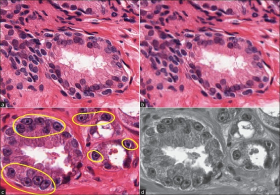
A tissue image region at (a) 20× and (b) 5× magnifications. In the high-magnification region, the tissue elements (nuclei, cytoplasm) are clearly visible. Two types of features considered in a tissue region are (c) cytological feature, which is the presence of cancer nuclei in the region; (d) textural features extracted from the grayscale intensity distribution of the region

Table 1.

Summary of major studies on ROI classification in automated prostate cancer diagnosis. Since different authors used different datasets, their results cannot be directly compared

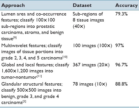
Figure 2.

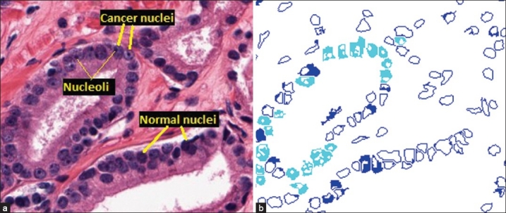
Nucleus segmentation and classification. (a) Cancer and normal nuclei in a 20× tissue region. (b) Results of the nucleus segmentation and classification. Cyan regions are cancer nuclei and blue regions are normal nuclei. The blank areas inside each nucleus region are the segmented dark spots obtained by the maximum object boundary binarization algorithm. In cyan regions, these spots are round and small in size, which are considered nucleoli. In blue regions, these spots are either elongated or much larger in size, which are not considered nucleoli

Figure 5.

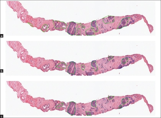
Detection results on a test image. The blue contour depicts the annotated cancer region by the pathologist and the green contours depict the outputs by the algorithm. (a) Result of the texture based method; (b) result of the cytological feature based method and (c) result of the proposed feature combination method. t_d = 90 pixels is used for all three methods

In the proposed approach, we first find all the cancer nuclei in the tissue. Then, we divide the image into a grid of patches. For each patch, we compute two types of features (cytological and textural features; [Figures 1c, 1d], and combine them to classify the patch as normal or cancerous. Finally, neighboring cancer patches are unified into continuous cancer regions.

NUCLEUS SEGMENTATION AND CLASSIFICATION

Nucleus Segmentation

To segment nuclei from the tissue area, we propose a maximum object likelihood binarization (MOLB) algorithm. Our goal is to segment an object O with feature vector ƒ(O) in a grayscale image I. We first assume that ƒ(O) follows a density g with parameter vector θ. An estimate is obtained from a training set. A threshold t₀ to binarize I is obtained such that the average object likelihood of the foreground blobs is maximized. Formally, let B^t_i, i = 1, . . . , n^t denote the n^t foreground blobs generated by binarizing I with a threshold t ∈ [t_min, t_max] (note that B^t_i and n^t depend on t). We choose t₀ such that

where ƒ(B^t_i) is the feature vector of blob B^t_i and is the object likelihood of blob B^t_i since it estimates how similar the features of B^t_i are to the features of the object of interest O (which have density g with parameter ).

In this procedure, after binarizing I using a threshold t ∈ [t_min, t_max], we apply a 4-connectivity connected component algorithm to group foreground pixels (pixels whose intensities are greater than t) into blobs B^t_i, i = 1, . . . ,n^t. This is followed by computation of blob features, ƒ(B^t_i), and their average object likelihood, . The optimal threshold t₀, computed in Equation (1), is the threshold resulting in the maximum average object likelihood. The blobs obtained by binarizing I with t₀ are the outputs of the algorithm.

Since nuclei appear as blue in H&E stained images, we apply this algorithm on the b channel (which is normalized to [0,1]) of the Lab color space (which best represents the blue color). Here, objects O to be segmented are the nuclei. The feature vector of the nucleus is defined as ƒ(O) = (a, c), where a and c denote the area and circularity of a nucleus, respectively. The circularity is defined as c = (4πα)/p², where p denotes the perimeter of the nucleus. In this problem, we assume that the feature density is bivariate Gaussian , where and are estimated from a training set of manually segmented nuclei.

NUCLEUS CLASSIFICATION

Nuclei in cancer glands[7,8] usually appear light blue and contain prominent nucleoli which appear as small dark spots. On the other hand, nuclei in normal glands usually appear uniformly dark or uniformly light over its entire area without the nucleoli [Figure 2a]. We utilize this observation to classify the segmented nuclei into normal or cancer nuclei. First, we segment the dark spots from each nucleus; then the features of these spots are used to determine if the nucleus is a cancer nucleus. These two operations are performed as follows.

Maximum Object Boundary Binarization

By observing that boundaries of the salient objects (dark spots) within a region of interest (nucleus region) typically have strong gradient magnitude, we find a threshold t₀ to binarize the ROI (in a grayscale image) in such a way that it generates the foreground object which has the maximum gradient magnitude on the boundary. Formally, let O^t_i i = 1, . . . , n^t, denote the n^t foreground objects obtained in the ROI, R, when binarizing R with a threshold t ∈ [t_min, t_max] (note that O^t_i and n^t depend on t). We choose t₀ such that

where bound_mag (O^t_i) denotes the average gradient magnitude of the pixels on the boundary of O^t_i.

In this procedure, after binarizing R using a threshold t ∈ [t_min, t_max], we use the 4-connectivity property to group foreground pixels (pixels whose intensities are greater than t) into objects O^t_i, i= 1, . . . , n^t. Then we compute the average gradient magnitude on the boundary of each object and get the maximum value of these average magnitudes . The best threshold t₀, which is computed in Equation (2), is the threshold that maximizes the object boundary gradient magnitude. This is a local binarization method since in each ROI, we find a different threshold t₀ to binarize and detect the local objects in that ROI.

Since the difference in intensity of the nucleolus and the rest of the nucleus area is most salient in the luminance channel of the image, we apply the algorithm in this channel to segment the dark spots. However, we obtain several spots in each nucleus because some noisy dark regions resulting from the poor tissue staining procedure may also generate spots. Figure 3 shows the result of this binarization.

Figure 3.

A cancer nucleus (left) and the segmented dark spots (right). There are two spots detected by the proposed algorithm, one is a true nucleolus and the other is a noisy spot

Feature-based Object Identification

We need to identify an object of interest O^* (nucleolus) among a pool of objects {O_i}ⁿ_i=1 (dark spots). Similar to the formulation of the MOLB algorithm in the previous section, we estimate the parameters of the density g of the feature vector ƒ(O^*) from a training set of manually segmented nucleoli. Then, we choose the object O_m which has the maximum likelihood: . The object O_m is considered the object of interest, where the constraints for each feature, i.e., ƒ^min_i < ƒ_i(O_m) < ƒ^max_i ∀j are estimated from the training set. We again use area and circularity as the features to identify the nucleoli. By using this algorithm, if a nucleolus is found within a nucleus, that nucleus is classified as a cancer nucleus. Otherwise, it is considered a normal nucleus. Figure 2b depicts the results of the nucleus segmentation and classification. For cancer detection purposes, we only keep cancer nuclei and disregard normal nuclei.

TEXTURAL FEATURES

Similar to Ref.[6], the textural features computed for an image patch include first-order statistics, second-order statistics, and Gabor filter features. There are four first-order statistical features comprising mean, standard deviation, median, and gradient magnitude of pixel intensity in the patch. For the second-order statistical features, we form the co-occurrence matrix for all the pixels in the patch and compute 13 features from this matrix[12] which include energy, correlation, inertia, entropy, inverse difference moment, sum average, sum variance, sum entropy, difference average, difference variance, difference entropy, and two information measures of correlation. For the Gabor filter-based texture features,[13] we create a bank of 10 filters by using two different scales and five different orientations. The mean and variance of the filter response are used as features. Thus, a total of 20 features are extracted by using Gabor filters. We obtain 37 features using these three feature types (4 first-order statistics features, 13 co-occurrence features and 20 Gabor features). By considering texture in each of the three normalized channels of the Lab color space of the image separately, we have a total of 3 × 37 = 111 textural features for each patch.

DETECTION ALGORITHM

Since we do not have any prior information (size, shape, and boundary) about the cancer regions, we utilize a patch-based approach using a feature set combination method to detect the cancer regions. A grid of patches, each with S × S pixels, is superimposed on the image. Let {x_i}ⁿ_i=1 denote the n sets of features associated with each patch P. Each set x_i may contain one or more features. We train n classifiers {ƒ_i}ⁿ_i=1, one for each feature set. A patch P is classified as a cancer patch if

where p(ƒ_i(x_i) = 0) and p(ƒ_i(x_i) = 1) denote the probability that classifier ƒ_i classifies the feature set x_i as normal or cancer, respectively. Otherwise, P is considered a normal patch. We apply this algorithm in our problem with two different feature sets (n=2), i.e., cytological feature set and textural feature set. The cytological feature set contains a single feature which is the number of pixels belonging to cancer nuclei in the patch. Both classifiers (ƒ₁ and ƒ₂) used for these two feature sets are Support Vector Machine (SVM) with RBF kernel and c = 1. The grid size and placement are chosen based on the method discussed in Ref.[6] where the authors superimposed the image with a uniform grid so that the image is divided into 30×30 regions. The reported result using this grid was better than that of the pixel-based method proposed in the same paper. In a similar manner, we divide the image into 40×40 patches (S = 40) and perform patch classification.

Once cancer patches are identified, we create continuous cancer regions by grouping neighboring cancer patches. We divide cancer patches in the image into groups, where each group O contains a set of cancer patches {P_i}^m_i=1 such that ∀P_i ∈ O, ∃P_j ∈ O, where d(P_i, P_j) ≤ t_d. Groups with a small number of patches are discarded. For each remaining group, we create one continuous cancer region by generating a convex hull of all the patches and set all pixels in this convex hull as cancer pixels. Cancerous tumors are characterized by uncontrolled growth, which makes the spread and shape of the tumor extremely difficult to model. We, therefore, take the most reasonable simplification, i.e., capture the convex hull to get all the cancer regions that may correspond to a single tumor. The grouping process and the removal of small groups (groups with small number of patches) follow the annotation strategy of the pathologist. We can observe in the ground truth that the pathologist only annotates large cancerous regions, including several neighboring cancerous glands but not individual glands. Hence, the minimum size of a group is chosen to be larger than the average size of a cancerous gland.

Many of the assessments made by pathologists are based on a gestalt of the entire region using years of training and experience in evaluating many tissues with cancer. For pathologists, this constitutes their “self evident truth” or heuristics that is usually not documented. The case when a pathologist identifies two neighboring regions as a single region and when he considers them two independent regions is very subjective. With the automated detection and grading research we are engaged in, we hope that some of the subjectivity will be codified and we will have a more consistent review and analysis of cancerous tissues.

EXPERIMENTS

Our dataset contains independent training and test sets. The training set includes six images (approximate size is 4,000×7,000 pixels at 20× magnification). In each training image, all the cancer glands were marked by a pathologist. In the remaining noncancerous area, we manually selected a number of training normal regions which contain various benign structures of the tissue (stroma, normal glands with different sizes, normal nuclei). Figure 4a shows part of a training image. The independent test set consists of 11 whole slide images at 20× magnification (approximate size is 5,000×23,000 pixels). The difference in size of the training and testing images is not an important issue because what we need for training is the local information of the patches but not the global information of the entire image. The ground truth for the test images (all cancer regions) were also manually labeled by a pathologist. All the nonlabeled regions are considered normal. While in the ground truth of the test set, the pathologist annotated the entire cancer region (including neighboring cancer glands and the intervening normal structures such as stroma), only pixels belonging to the cancer glands are annotated as cancer in the training set. In other words, the training data are more reliable.

Figure 4.

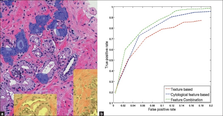
Experimental results. (a) A region of a training image in which cancer gland regions are highlighted in blue and selected normal regions are highlighted in yellow. (b) ROC curves, which plot the average FPR vs. TPR over all test images, for the proposed feature combination method, the texture based method and the cytological feature based method obtained by varying the neighboring threshold t_d from 0 pixels to 530 pixels. Note that the scales for TPR and FPR are different

To evaluate the robustness of the cytological feature as well as of the proposed feature combination method, we compare the performance of the three methods, i.e., the feature combination method, the texture based method and the cytological feature based method. In the texture based method, we only use the textural feature set (section 4) and a single classifier (SVM with RBF kernel and c = 1) for the detection. Similarly, we only use the cytological feature set for the cytological feature based method. For a quantitative comparison, we compute the true positive rate TPR = TP/(TP + FN) and the false positive rate FPR = FP/(TN + FP), where TP, FP, TN, and FN denote the true positive, false positive, true negative, and false negative, respectively, for every test image. The TPR and FPR are then averaged over all test images.

The value of the threshold t_d has a significant influence on both TPR and FPR. Since the training set only includes annotations of cancer glands separately and not the entire cancer region, it is difficult to estimate t_d. Further, it is difficult for a pathologist to tell which value he uses to annotate the cancer region. Hence, it is necessary to test all methods with different values of t_d. Figure 4b depicts the ROC curves illustrating the relationship between TPR and FPR obtained by the three methods when t_d is varied from 0 pixels to 530 pixels (a relatively large distance in the image). When t_d increases, both TPR and FPR increase, i.e., there are more true cancer regions being detected while at the same time, more normal regions get incorrectly classified as cancer. For the same FPR, the feature combination method always gets a higher TPR than the other two methods. Since the test set is not large, we choose the best trade-off between TPR and FPR by a qualitative observation of the detection outputs. We determine that for t_d = 90 pixels, the feature combination method provides the most satisfactory detection results (TPR = 78% at FPR = 6%). Figure 5 shows the detection results of the three methods on a whole slide image when t_d = 90 pixels and Figure 6 shows a close-up region of the same image for better details. In this image, all three methods can find most of the cancer regions. However, the feature combination method has fewer false detections than the other two methods.

Figure 6.

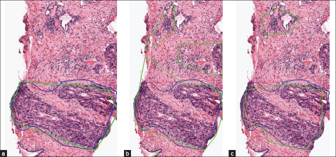
Detection results of the proposed feature combination method (a), the texture based method (b), and the cytological feature based method (c) in a close-up region sampled from the images in Figure 5

To save computation time, we perform background removal by using a simple thresholding operation on the L channel of the Lab color space. By doing this, the white area (non-tissue area) is discarded prior to the patch feature extraction. However, to be able to compare our results with reference[5,6] in which the authors did not perform background removal, we use all the image pixels when computing the TPR and the FPR. Although different datasets were used, we can still have an indirect comparison among the three studies. At a TPR of 87% (which was the most satisfactory result in Ref.[5]), the FPR obtained by their method was roughly 10%, in Ref.[6] it was roughly 28% and in the proposed feature combination method it is roughly 9%. In the context of this paper, since we use background removal for all three methods (texture based, cytological feature based and feature combination methods) and compute the TPR and the FPR for them in the same way, the comparison among these three methods is still valid.

We do not compare our selected features with morphological features because, to compute morphological features, we need to segment complete glands, which is not a trivial task. Since we do not have ground truth for the nucleus segmentation (it is indeed a labor intensive task for pathologists to mark every single nucleus), we only qualitatively evaluate the proposed nucleus segmentation method (the MOLB method) by comparing with the popular Otsu's method[14] and a Bayesian classification method which was used in reference.[15] Otsu's method is an adaptive thresholding method which is used to create a binary image I_b from a grayscale image I_g. This method assumes that each image pixel belongs to one of the two classes, i.e., foreground and background. Then, it searches for an optimal threshold t₀ ∈ [a, b], where [a, b] is the intensity range of I_g, to binarize I_g such that the interclass variance is maximized. The interclass variance corresponding to a threshold t is computed by

σ²_b(t)=ω₁(t)ω₂(t)[μ₁(t)–μ₂(t)²]      (4)

where ω₁, ω₂ denote the probabilities and μ₁, μ₂ denote the intensity means of the two classes. We apply Otsu's method on the b channel of the Lab color space to obtain pixels belonging to the nuclei (foreground pixels). In their Bayesian method, Naik et al.[15] obtained training pixels of three different tissue classes which are lumen, nucleus and cytoplasm. For each class ω_v, they learned a probability density function p(c, ƒ(c)|ω_v for a pixel c with color ƒ(c). By using Bayes Theorem, they computed the posterior probability P(ω_v|c, ƒ(c)) that each pixel c belongs to each class ω_v in the image. A pixel c is classified as nucleus if P(ω_N |c, ƒ(c)) > T_N where ω_N denotes the nucleus class and T_N denotes a pre-defined threshold. Since we cannot estimate the threshold T_N being used in their method, we classify a pixel c as nucleus if P(ω_N|c, ƒ(c)) > P(ω_C|c, ƒ(c)) and P (ω_N|c, ƒ(c)) > P(ω_L|c, ƒ(c)), where ω_C and ω_L denote the cytoplasm and lumen classes, respectively. Similar to their work, we use 600 pixels per class for training. The results of the three methods are presented in Figure 7. It can be seen from these results that the MOLB method gives more satisfactory outputs than the other two methods. While the Otsu method does not employ any domain knowledge and the Bayesian method may suffer from the high color variation of the tissue structures among images, the MOLB method uses prior knowledge about nucleus features (which are mostly stable among images) and does not depend on color of some training pixels.

Figure 7.

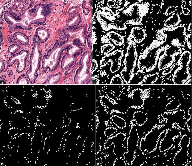
Comparison of the three nucleus segmentation methods. (a) A sampled region of a whole slide image. (b) Result of the Otsu method. (c) Result of the Bayesian method. (d) Result of the MOLB method

We also analyze the computational complexity of the MOLB algorithm by calculating the number of operations to be performed. There are three steps in this algorithm: (i) thresholding the grayscale image with a threshold t, (ii) performing the connected component labeling using all image pixels and (iii) computing features of the objects (connected components). These three steps are repeated for all T threshold values in [t_min, t_max]. In the thresholding step, there are n comparisons for an image with n pixels, yielding a complexity of Θ(n). In the connected component labeling, by using a two-pass algorithm (every pixel is visited twice) with 4-connectivity at every pixel, 2×4×n operations are needed, which corresponds to a complexity of Θ(n). To compute features (area and circularity) of each segmented object O_i with n_i points, we need to visit all the points and consider the four neighbors at every point to find the object perimeter, which results in 4n_i operations. The total number of operations for this step is Σ_i4n_i, which corresponds to a complexity of Θ(Σ_i4n_i) = Θ(4n) = Θ(n) (since Σ_in_i<n). In summary, the final complexity of the algorithm is T ×(Θ(n) + Θ(n) + Θ(n)) = Θ(n), which is linear in terms of the number of pixels in the image.

CONCLUSIONS

We have introduced a novel cytological feature for automated prostate cancer detection, which is different from the structural features used in the Gleason grading method. An efficient adaptive binarization approach is proposed to extract this cytological feature, namely the cancer nucleus feature. Though the Gleason grading method is widely used in grading prostate cancer, there is still a need to examine the tissue at a high magnification and utilize the cytological features to enhance the diagnosis results. For a computer aided system, besides the use of well-known textural features, we can also include the cancer nucleus feature in particular and cytological features in general to boost the performance of the system. The results achieved on the test images reported here demonstrate the contribution of the cancer nucleus feature in detecting prostate cancer. In future work, we intend to obtain a larger dataset and explore additional cytological features. Moreover, we plan to perform gland segmentation and use the outputs to facilitate cancer detection. This means we can process cancer detection at a higher level (glandular level) instead of patch-based classification which relies mainly on image pixels.

REFERENCES

- 1.Kiernan JA. London: A Hodder Arnold Publication; 2001. Histological and Histochemical Methods: Theory and Practice. [Google Scholar]
- 2.Gleason D. Histologic grading and clinical staging of prostatic carcinoma. In: Tannenbaum M, editor. Urologic Pathology: The Prostate. Philadelphia, PA: Lea and Febiger; 1977. pp. 171–98. [Google Scholar]
- 3.Nguyen K, Jain A, Allen R. Automated gland segmentation and classification for Gleason grading of prostate tissue images. Proc. International Conf. Pattern Recognition. 2010:1497–500. [Google Scholar]
- 4.Gong Y, Caraway N, Stewart J, Staerkel G. Metastatic ductal adenocarcinoma of the prostate: cytologic features and clinical findings. J Clin Path. 2006;126:302–9. doi: 10.1309/4TT6-LVJP-QVFW-DB6P. [DOI] [PubMed] [Google Scholar]
- 5.Monaco JP, Tomaszewski JE, Feldman MD, Hagemann I, Moradi M, Mousavi P, et al. High-throughput detection of prostate cancer in histological sections using probabilistic pairwise markov models. Med Image Anal. 2010;14:617–29. doi: 10.1016/j.media.2010.04.007. [DOI] [PMC free article] [PubMed] [Google Scholar]
- 6.Doyle S, Feldman M, Tomaszewski J, Madabhushi A. A boosted bayesian multi-resolution classifier for prostate cancer detection from digitized needle biopsies. IEEE Transactions on Biomedical Engineering. 1990:581–90. doi: 10.1109/TBME.2010.2053540. [DOI] [PubMed] [Google Scholar]
- 7.Mason M. Cytology of the prostate. J Clin Path. 1964:581–90. doi: 10.1136/jcp.17.6.581. [DOI] [PMC free article] [PubMed] [Google Scholar]
- 8.Diaconescu S, Diaconescu D, Toma S. Nucleolar morphometry in prostate cancer. Bull Transilvania Univ Brasov 3. 2010 [Google Scholar]
- 9.Diamond J, Anderson N, Bartels P, Montironi R, Hamilton P. The use of morphological characteristics and texture analysis in the identification of tissue composition in prostatic neoplasia. Human Pathology. 2004;35:1121–31. doi: 10.1016/j.humpath.2004.05.010. [DOI] [PubMed] [Google Scholar]
- 10.Khouzani KJ, Zadeh HS. Multiwavelet grading of pathological images of prostate. IEEE Trans Biomed Eng. 2003;50:697–704. doi: 10.1109/TBME.2003.812194. [DOI] [PubMed] [Google Scholar]
- 11.Tabesh A, Teverovskiy M, Pang HY, Kumar VP, Verbel D, Kotsianti A, et al. Multifeature prostate cancer diagnosis and gleason grading of histological images. IEEE Trans Med Imaging. 2007;26:1366–78. doi: 10.1109/TMI.2007.898536. [DOI] [PubMed] [Google Scholar]
- 12.Haralick R, Shanmugam K, Dinstein I. Textural features for image classification. IEEE Trans Syst Man Cybern SMC. 1973;3:610–21. [Google Scholar]
- 13.Jain AK, Farrokhnia F. Unsupervised texture segmentation using gabor filters. Pattern Recognit. 1991;24:1167–86. [Google Scholar]
- 14.Otsu N. A threshold selection method from gray-level histograms. IEEE Trans Sys Man Cyber. 1979;9:62–6. [Google Scholar]
- 15.Naik S, Doyle S, Feldman M, Tomaszewski J, Madabhushi A. Gland segmentation and computerized gleason grading of prostate histology by integrating low-, high-level and domain specific information. MIAAB Workshop. 2007 [Google Scholar]