A comparison of sampling strategies for histological image analysis

Abstract

Histological image analysis methods often employ machine-learning classifiers in order to adapt to the huge variability of histological images. To train these classifiers, the user must select samples of the relevant image objects. In the field of active learning, there has been much research on sampling strategies that exploit the uncertainty of the current classification in order to guide the user to maximally informative samples. Although these approaches have the potential to reduce the training effort and increase the classification accuracy, they are very rarely employed in practice. In this paper, we investigate the practical value of uncertainty sampling in the context of histological image analysis. To obtain practically meaningful results, we have devised an evaluation algorithm that simulates the way a human interacts with a user interface. The results show that uncertainty sampling outperforms common random or error sampling strategies by achieving more accurate classification results with a lower number of training images.

INTRODUCTION

One of the biggest challenges in the analysis of histological whole-slide images is the huge variability of the visual appearance within and across slides. For this reason, many image analysis approaches employ machine-learning classifiers that can be adapted to varying image characteristics simply by giving examples of the relevant image objects. Image objects, in this sense, are nuclei, cells or tissue regions with certain cellular patterns. The performance of machine-learning classifiers is heavily dependent on the sample objects on which they are trained. Yet, the practical issue of sample selection is often ignored. Most publications on adaptive histological image analysis methods simply assume fixed sets of preclassified image objects on which the classifier is trained and fixed sets on which its performance is tested.[1–4] In actual applications, though, the user must be able to continually improve the classifier by selecting further image object samples when the accuracy on novel images is insufficient.[5]

There are different strategies for carrying out the sample selection process. Since the selection of image object samples requires considerable effort by the user, a good sampling strategy should encourage the selection of maximally informative samples and, thereby, minimize the number of samples required to achieve a certain accuracy. At the same time, the sampling strategy should be simple and intuitive so that the user can operate it without comprehensive instructions. In random sampling, image object samples are selected by pure chance. In error sampling, the user subjectively selects image object samples that were incorrectly classified. Its simplicity and intuitive usage make error sampling the most common sampling strategy applied in practice. Both random and error sampling are examples of passive learning because the selection of samples is driven by the user. Recently, however, there is growing research on active learning strategies that actively query the most informative samples from the user in order to optimize the classification model.[6] Most active learning strategies rely on an informativeness measure in order to prioritize samples. While a wealth of informativeness measures has been proposed in the literature, the most simple and widely used measure remains the classification uncertainty[6] which is generally derived from the disparity between individual class weights.

Although many studies have shown that active learning can achieve better classification results with a lower number of training samples, it is still rarely applied in practice. In fact, a recent survey on the usage of active learning in natural language processing revealed widespread skepticism about its practical utility.[7] Compared with passive learning, active learning both requires additional implementation effort and complicates the user interface. To answer whether the benefit of uncertainty sampling justifies its overhead, this paper performs a comparison of different sampling strategies in the context of histological image analysis.

In order to perform the comparison in an objective and practically meaningful way, we have devised an evaluation algorithm for sampling strategies that simulates the way a human interacts with a user interface. In contrast to most evaluations performed in the active learning literature, our algorithm does not select image objects from the total population of possible appearances. Instead, it successively selects samples from single images which corresponds to the usual workflow in practical histological image analysis applications. Furthermore, in the literature, uncertainty sampling is most often evaluated among other active learning strategies or random sampling.[8,9] For a reasonable assessment of its practical value, however, uncertainty sampling must be compared with error sampling. To enable the simulation of passive sampling strategies like error sampling, our evaluation algorithm assumes a “relaxed” scenario of active learning. Instead of directly querying the user for certain image object samples, the user can freely choose among all image objects from the current image and is merely encouraged to prioritize some objects over others. We have implemented the evaluation algorithm on the basis of an existing method for quantifying necrosis in histological whole-slide images and applied it to two image sets. The results demonstrate the superiority of uncertainty sampling over other sampling strategies and error sampling in particular.

MATERIALS AND METHODS

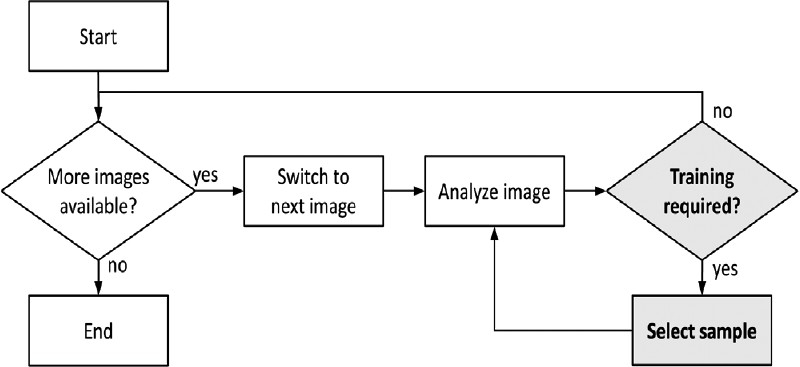
The training process of adaptive image analysis applications can be summarized in the following general workflow [Figure 1]. First, the user chooses an image set to work on and switches to the first image. Then, the user triggers the analysis of the first image. If the result is satisfactory the user will directly proceed to the next image. If, however, the user feels that the image needs more training, the user will designate the class of certain image objects and request an update of the classification model. Then, the analysis will be executed again in order to see the updated classification result. This loop of image analysis and sample selection is repeated until the image does not require any more training and the next image can be analyzed. In a semiautomated usage scenario, this workflow is continued until all images have been processed. In a fully automated usage scenario, this workflow is executed on a small number of training images in order to gain a robust classification model that can be applied to new images without any further interaction.

Figure 1.

Most adaptive image analysis applications are based on the depicted workflow. The main image analysis algorithm is executed in the step “Analyze Image” while the steps “Training required?” and “Select sample” represent the sampling process. In this paper, we compare different sampling strategies through different implementations of these two items

This general workflow can be easily translated into an algorithm that simulates the way a human interacts with an adaptive image analysis application. For this purpose, each of the steps depicted in Figure 1 is implemented by a different function. The function “Analyze image” implements the main image analysis algorithm. The functions “Training required?” and “Select sample”, on the other hand, represent the applied sampling strategy. It is the task of the “Training required?” function to decide whether the training process of the current image should be continued. The function “Select sample” selects additional sample image objects from a predefined ground-truth classification of the current image.

In this paper, we simulate different sampling strategies through different implementations of the “Training required?” and “Select sample” functions. The “Analyze image” function, in this case, is implemented on the basis of an existing algorithm for the quantification of necrosis in histological whole-slide images. This algorithm divides the image into a regular grid of square image objects and classifies each of them as either viable tissue, necrotic tissue or background. The classification is performed by a Random Forest classifier[10] on the basis of different spectral and textural features. The spectral features include the min, max, mean, standard deviation, quartiles and the median of the intensity distribution in the red, green and blue color channels. To save computing time, they are extracted at a low magnification of 12.5×. The texture features, on the other hand, are extracted at a high magnification of 50× that is able to resolve fine spatial structures. The texture features comprise local binary patterns[11] in an 8-neighborhood that are extracted from the red color channel. The algorithm incorporates a standard Random Forest classifier without online-learning capabilities that is completely retrained whenever the sample set changes.

Random Sampling

Obviously, the simplest sampling strategy is to select a fixed number of random samples per image. In a user interface, such a strategy could be implemented by highlighting a predefined set of random image objects that the user has to classify manually. To simulate this, we have implemented a sampling strategy called Random, where the function “Select sample” just adds one random object to the classification model and where the function “Training required?” simply checks whether a minimum number of 15 samples per image has been reached.

Error Sampling

The main problem of the Random strategy is that it does not take the current classification error into account. The classification error, however, provides valuable information on the minimum number of required samples and the prioritization of new samples. A user interface for an error sampling strategy has to provide the possibility to compare the current classification result with the original image, so that the user can identify mistakes. Then, the user can decide whether the current classification quality is sufficient or select further samples from the class that produces the most errors. We have implemented two error sampling strategies which are called Error and Error Min. The only difference is that the Error Min strategy requires a minimum number of samples per image while the Error strategy aborts the training process as soon as the classification quality is sufficient.

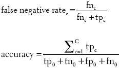
Both strategies rely on two statistics. The false negative rate of class c quantifies the error caused by falsely not classifying image objects as that class. The accuracy, on the other hand, is a class-independent measure for the overall classification quality. For the computation of these statistics, the total number of image objects is divided into true positive tp_c, true negative tn_c, false positive fp_c, and false negative fn_c cases for each class c:

In both error strategies, the “Select sample” function selects one image object from the class with the maximum false negative rate:

c=argmax_{c∈{1,…,C}} false negative rate_c

The “Training required?” function of the Error strategy simply checks whether the accuracy exceeds a threshold of 0.92 which is assumed to signify a satisfactory classification result. The strategy Error Min extents this requirement by the further condition that at least 15 samples are chosen per image.

Uncertainty Sampling

In addition to the described common sampling strategies, we have also implemented a more sophisticated strategy which exploits the uncertainty of the current classification. For the quantification of uncertainty we assume that the classification algorithm does not only assign a definite class to a given image object, but individual weights ω_c that quantify the confidence that an image object belongs to class c. The definite class is then simply determined as the one with the maximum weight (argmax_{c∈{1,....C}} ω_c). When the weight of the definite class does not achieve a two-thirds majority over the other class weights, we consider the classification to be uncertain:

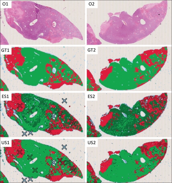
We have created a user interface that enables uncertainty sampling for the necrosis quantification method that serves as the example application in this paper. The main component of this user interface is a full-featured virtual microscope viewer, where the user can arbitrarily pan and zoom through the current image. At any time, the current classification result is visualized as a colored overlay on top of the original image. In this overlay, all image objects are filled with a color representing their classification, with “viable”, “necrotic” and “background” objects being drawn in green, red, and blue, respectively. During the training process, the user is encouraged to select both samples of falsely classified image objects and of those that are uncertainly classified. While the former can be identified by changing the opacity of the classification visualization, the latter can be easily recognized because they are drawn in a darker color. The training process is supposed to be performed until both the number of falsely and uncertainly classified image objects becomes negligible [Figure 2].

Figure 2.

Uncertainty sampling by the example of an image analysis method for quantifying necrosis. The images O1 and O2 show rat liver sections affected by confluent necrosis. To quantify the proportion of necrotic tissue, each section is divided into square image objects that are classified as either “viable tissue” (green), “necrotic tissue” (red) or “background” (blue). The images GT1 and GT2 show the respective ground-truth classifications provided by a human expert. Image ES1 shows the classification result after error sampling. Although the result already closely resembles the ground truth, many image objects are still uncertainly classified, as indicated by the darker color. Image US1 shows the classification result after uncertainty sampling. Although the selection of three additional samples has no major impact on the classification quality, it reduces the overall uncertainty to a negligible level. In the images ES2 and US2, the respective classification models obtained from ES1 and US1 were applied to the second section without modification. Obviously, uncertainty sampling both improved the classification accuracy and confidence

In order to simulate uncertainty sampling, we have implemented the sampling strategy Uncertainty on the basis of two statistics. The uncertainty rate of class c quantifies the respective fraction of image objects that are uncertainly classified. The uncertainty, on the other hand, is a class-independent measure of the overall uncertainty of the current classification. Both statistics incorporate u_c, that is, the total number of uncertainly classified image objects of class c:

The “Select sample” function of the Uncertainty strategy selects one image object from the class with the maximum false negative rate or uncertainty rate:

c=argmax_{c∈{1,…,C}} max (false negative rate_c, uncertainty rate_c)

The “Training required?” function is similar to the one of the error strategies, in that it requires a minimum accuracy of 0.92, but, in addition, it also requires a negligible uncertainty value of less the 0.08.

RESULTS

We have simulated the different sampling strategies with two sets of histological whole-slide images. Both sets show Hematoxylin-Eosin stained sections of rat liver tissue with different amounts of confluent necrosis. Image set 1 comprises 12 images with sizes between 2.6 and 5.1 gigapixels. Image set 2 comprises 24 images with sizes between 1.2 and 3.7 gigapixels. Each image is accompanied by a ground-truth classification by a human expert that is used to determine the classification accuracy and to select training samples. On a standard notebook computer, the initial analysis of the images, including the feature extraction, always took less than 2 minutes per image. By contrast, the update of the classification model and the reanalysis of the image after a training step always took less than 1 second.

The simulation assumes a fully automated usage scenario. Therefore, the training process was executed with only a subset of the available images and the remaining images were used for evaluating the performance of the generated classification model. Each sampling strategy was simulated with different numbers of training images in order to assess the corresponding impact on the performance. To increase the validity of the results, each combination of sampling strategy and number of training images was simulated with 50 different subsets of images. In total, this resulted in 3600 runs of the simulation algorithm.

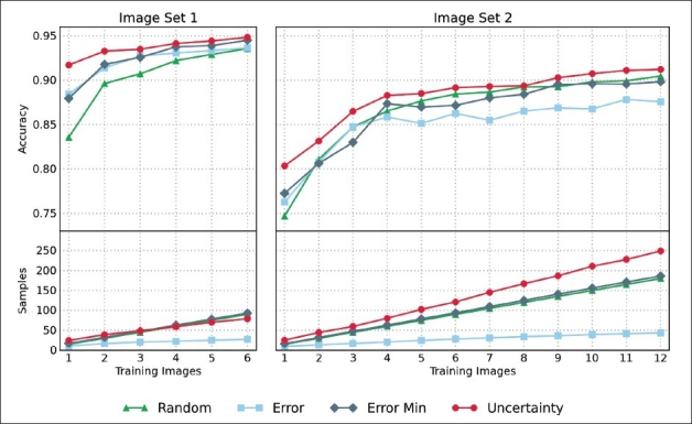
The simulation results are depicted in Figure 3. In both image sets, the mean accuracy improves with the number of training images, although the improvement decreases continually until the mean accuracy converges to an almost constant level. At the same time, the number of samples grows linearly with the number of training images for both image sets and all sampling strategies.

Figure 3.

The results of the training simulation. The left column shows the results for image set 1, the right column shows the results of image set 2. The upper row plots the number of training images against the respective mean accuracy of the generated classification model. The lower row plots the number of training images against the respective mean number of samples that were selected during the training process

In both image sets, the strategy Error caused the least number of samples to be selected. While its accuracy values are comparable to the Error Min strategy in the first image set, it is outperformed by the Error Min strategy in the second image set. Obviously, the minimum number of samples required by the Error Min strategy creates a more robust classification model.

Nevertheless, it appears to be impossible to define an optimal number of samples per image that works for all image sets. Image set 2 generally achieves worse mean accuracy values than image set 1. This indicates that the second image set requires a more complex classification model than the first one. The only strategy that adapts to these requirements is the Uncertainty strategy. While the other three strategies select an approximately equal number of samples per image in both image sets, the strategy Uncertainty selects about 39% more samples in the second set than in the first.

Independent of the number of training images, the strategy Uncertainty consistently produced the most accurate results for both image sets. This, however, cannot solely be attributed to the increased number of samples per image. In image set 1, the strategy Uncertainty clearly outperforms the other strategies although the number of samples is on par with the strategies Random and Error Min. Obviously, the strategy Uncertainty also selects more informative samples that produce a more robust classification model. Intuitively this makes sense. The uncertainly classified image objects are the ones that lie close to the current decision boundary of the classifier. By providing these image objects as training samples, the classifier can refine its decision boundaries much more effectively than with samples from arbitrary positions in the feature space.

CONCLUSION

In this paper, we have compared different sampling strategies for adaptive histological image analysis. The particular aim of the study was to determine whether the commonly employed error sampling strategy can be improved through uncertainty sampling and whether the benefit justifies the overhead. In order to answer this question from a practical point of view, we have devised an evaluation algorithm that simulates the way a human interacts with a user interface. The different strategies were evaluated on the basis of an image analysis method for the quantification of necrosis and applied to two sets of histological whole-slide images. In both cases, the uncertainty strategy outperformed the other strategies by consistently achieving higher accuracy values with a lower number of training images. Obviously, due to its limited scope, our study does not prove that uncertainty sampling is beneficial in all scenarios of adaptive histological image analysis. Further research needs be carried out on the effects of different classification algorithms, image sets, and informativeness measures. Likewise, the results do not enable predictions of the number of training images required to achieve a given accuracy. The results do show, however, that uncertainty sampling can considerably reduce the training effort by the user and improve the overall classification accuracy. Since uncertainty sampling can be intuitively integrated in a user interface by drawing uncertainly classified image objects in a darker color, it does not significantly increase the complexity of the user interface. In the same way as in the fully automated usage scenario, uncertainty sampling will be applicable in semiautomated usage scenarios as well. Since our evaluation is based on standard methodologies, we expect that there are a great number of applications in histological image analysis where uncertainty sampling will be beneficial.

REFERENCES

- 1.Diamond J, Anderson NH, Bartels PH, Montironi R, Hamilton PW. The use of morphological characteristics and texture analysis in the identification of tissue composition in prostatic neoplasia. Hum Pathol. 2004;35:1121–31. doi: 10.1016/j.humpath.2004.05.010. [DOI] [PubMed] [Google Scholar]
- 2.Mete M, Xu X, Fan CY, Shafirstein G. Automatic delineation of malignancy in histopathological head and neck slides. BMC Bioinform. 2007;8(Suppl 7):S17. doi: 10.1186/1471-2105-8-S7-S17. [DOI] [PMC free article] [PubMed] [Google Scholar]
- 3.Petushi S, Garcia FU, Haber MM, Katsinis C, Tozeren A. Large-scale computations on histology images reveal grade-differentiating parameters for breast cancer. BMC Med Imaging. 2006;6:14. doi: 10.1186/1471-2342-6-14. [DOI] [PMC free article] [PubMed] [Google Scholar]
- 4.Sertel O, Kong J, Shimada H, Catalyurek UV, Saltz JH, Gurcan MN. Computer-aided prognosis of neuroblastoma on whole-slide images: Classification of stromal development. Pattern Recogn. 2009;42:1093–103. doi: 10.1016/j.patcog.2008.08.027. [DOI] [PMC free article] [PubMed] [Google Scholar]
- 5.Fuchs J, Buhmann JM. Computational pathology: Challenges and promises for tissue analysis. Comput Med Imaging Graph. 2011;35:515–30. doi: 10.1016/j.compmedimag.2011.02.006. [DOI] [PubMed] [Google Scholar]
- 6.Settles B. Active Learning Literature Survey. Computer Sciences Technical Report 1648, University of Wisconsin Madison. 2009 [Google Scholar]
- 7.Tomanek K, Olsson F. Workshop on Active Learning for NLP. Boulder, Colorado, USA: ACL Press; 2009. A web survey on the use of active learning to support annotation of text data. Proc. 2009. [Google Scholar]
- 8.Lindenbaum M, Markovitch S, Rusakov D. Selective sampling for nearest neighbor classifiers. Mach Learn. 2004;54:125–52. [Google Scholar]
- 9.Schein AI, Ungar LH. Active learning for logistic regression: An evaluation. Mach Learn. 2007;68:235–65. [Google Scholar]
- 10.Breiman L. Random Forests. Mach Learn. 2001;45:5–32. [Google Scholar]
- 11.Ojala T, Pietkäinen M, Mäenpää T. Multiresolution Gray-Scale and Rotation Invariant Texture Classification with Local Binary Patterns. IEEE Trans Pattern Anal Mach Intell. 2002;24:971–86. [Google Scholar]