Graphical processing unit implementation of an integrated shape-based active contour: Application to digital pathology

Abstract

Commodity graphics hardware has become a cost-effective parallel platform to solve m any general computational problems. In medical imaging and more so in digital pathology, segmentation of multiple structures on high-resolution images, is often a complex and computationally expensive task. Shape-based level set segmentation has recently emerged as a natural solution to segmenting overlapping and occluded objects. However the flexibility of the level set method has traditionally resulted in long computation times and therefore might have limited clinical utility. The processing times even for moderately sized images could run into several hours of computation time. Hence there is a clear need to accelerate these segmentations schemes. In this paper, we present a parallel implementation of a computationally heavy segmentation scheme on a graphical processing unit (GPU). The segmentation scheme incorporates level sets with shape priors to segment multiple overlapping nuclei from very large digital pathology images. We report a speedup of 19× compared to multithreaded C and MATLAB-based implementations of the same scheme, albeit with slight reduction in accuracy. Our GPU-based segmentation scheme was rigorously and quantitatively evaluated for the problem of nuclei segmentation and overlap resolution on digitized histopathology images corresponding to breast and prostate biopsy tissue specimens.

INTRODUCTION

In the rapidly developing field of digital pathology,[1] ability to accurately segment structures on digitized histology images, especially the ability to deal with overlapping and occluded structures, is highly critical in the context of a number of different diagnostic and prognostic applications.[2,3] In the context of prostate cancer (CaP) and breast cancer (BC), digitized hematoxylin and eosin (H and E)-stained tissue samples are often characterized by the presence of densely packed nuclei, in which overlap between two or more nuclei has proven to be a significant challenge to computerized segmentation schemes.[1–3] Shape-based active contours (level sets) have emerged as one of the natural solutions to overlap resolution. Recently, Ali et al.[3] proposed a shape-based hybrid active contour model that can segment all of the overlapping and nonoverlapping nuclei simultaneously in an image.

While level sets have found wide applicability for medical image segmentation, their clinical utility has been limited by (1) the amount of time needed for computation and (2) a number of free parameters that must be fine tuned for each specific application. These two limitations are intertwined, whereby users find it impractical to explore the entire space of possible parameter settings when an example result from a point in that space requires minutes or hours to generate. We have previously addressed the latter issue by automating the parameter selection associated with initialization.[3]

Higher level segmentation approaches, such as deformable models, have been ported to GPU architectures by considering implicit deformable models such as image lattices (e.g., a 2D curve is implicitly represented as the iso-value of a field encoded as a 2D image). Level-set approaches have become particularly popular in the GPU-segmentation community as significant speedups and interactive rendering have become available.[4,5] Geodesic active contours, which are a combination of traditional active contours (snakes) and level-set evolution, were efficiently implemented in GPU by using the total variational formulation and used primarily to separate foreground and background structures in 2D images.[6] These implementations were, however, designed for the evolution of a single level set.

In this paper, we present a novel, computationally efficient framework for segmentation of histologic structures (e.g., nuclei and glands) in very large histopathology images. The framework presented alleviates the computational overhead of level set segmentation by marrying a very fast solver with an intuitive speed function. We leverage a powerful graphical processing unit (GPU) (via commodity graphics hardware) to provide a computationally optimized segmentation framework that allows for simultaneous calculation of multiple, interacting level sets. We demonstrate an application of our parallelized framework using our previously published synergistic active contour models (using multiple level sets)[3,7] for the problem of segmenting nuclear and glandular structures on digitized histopathology. We have previously shown that this scheme[3,7] allows for accurately detecting and segmenting overlapping lymphocytes and nuclei in H and E-stained prostate and breast needle core biopsy images. Following are the main contributions of this work:

• A GPU accelerated multiple level set-based hybrid active contour framework, implemented using the NVIDIA CUDA libraries, for the task of rapid segmentation of nuclei in H and E images.

• Leveraging a parallelizable framework to accommodate multiple level sets operating in parallel with initialization via shape prior in conjunction with boundary and region-based energy terms.

• Exploit parallelism and efficient memory management in the GPU to achieve massive speedup compared to using a CPU.

The rest of the paper is structured as follows. Overview of GPU structure and programming paradigms are presented in section 2. Section 3 describes our segmentation algorithm. In Section 4 we describe our GPU-based framework and its implementation on graphics hardware. We present our analysis of the results in section 5. In section 6 we present our concluding remarks and discuss future improvements of our GPU-based implementation.

OVERVIEW OF GPGPU

General purpose computation on graphics processing units (GPGPU) is the technique of using graphics hardware to compute applications typically handled by the central processing unit (CPU). Graphics cards over the past two decades have been required to become highly efficient at rendering increasingly complex 3D scenes at high frame rates. This has forced their architecture to be massively parallel in order to compute graphics faster compared to general purpose CPUs.[4] GPUs are not optimized for general purpose programs, and thus lack the complex instruction sets and branch control of the modern CPU. Although current high-performance CPUs feature multiple cores for limited parallel processing, GPUs are arguably a more attractive option in terms of lower price and power usage.

Recently, languages have been developed that allow the programmer to implement algorithms without any knowledge of graphics application programming interface (APIs) or architectures The GPGPU computations performed in this work utilize the NVIDIA CUDA (Compute Unified Device Architecture) technology.[8] The C language model has at its core three key abstractions:[9] a hierarchy of thread groups (to allow for transparent scalability), shared memories (allowing access to low-latency cached memory), and barrier synchronization (to prevent race conditions). This breaks the task of parallelization into three subproblems, which allows for language expressivity when threads cooperate, and scalability when extended to multiple processor cores. CUDA allows a programmer to write kernels that when invoked execute thousands of lightweight identical threads in parallel. CUDA arranges these threads into a hierarchy of blocks and grids, as can be seen in Figure 1, allowing for runtime transparent scaling of code within GPU. The threads are identified by their location within the grid and block, making CUDA perfectly suited for tasks such as level set-based image segmentations where each thread is easily assigned to an individual pixel or voxel.[10]

Figure 1.

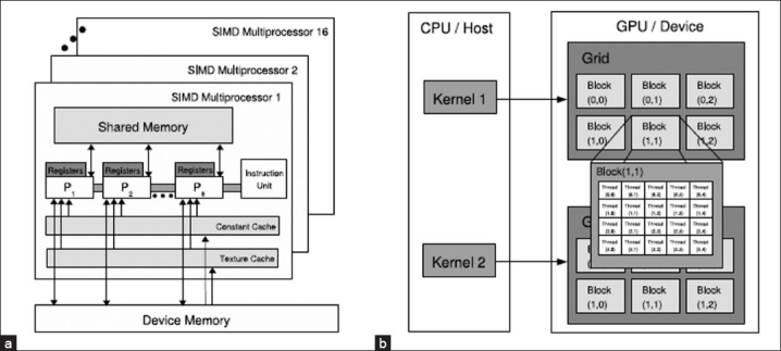
GPU architecture; (a) CUDA hardware interface, (b) CUDA software interface

NUMERICAL MODELING OF THE SEGMENTATION SCHEME

We present a slightly modified version of the previously published method by Ali et al.[7] for the problem of segmenting nuclei and lymphocytes in prostate and breast cancer images. Our previous model comprised a hybrid active contour (boundary and region based) integrated with the shape prior. In this work, we eliminate the boundary-based term in order to simplify the numerical modeling of the variational formulation of the hybrid active contour formulation, relying instead on the region and shape prior terms within a multiple level set formulation. Figure 2 illustrates the individual modules comprising the scheme.

Figure 2.

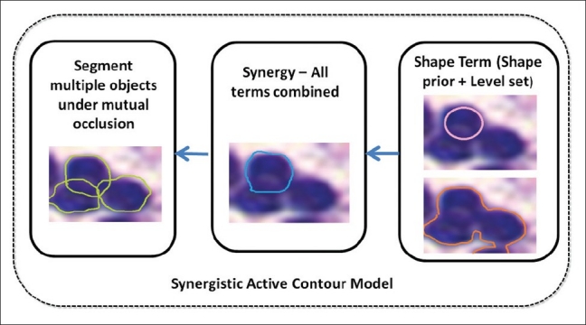
Flow chart showing the various modules comprising our segmentation scheme. First panel illustrates shape prior and region-based term. Second panel illustrates the synergy of both the terms

Integrated Shape-based Active Contour

We combine shape force and region force (Chan-Vese)[11] into a variational formulation:

where β_s, β_r > 0 are constants that balance contributions of the shape prior and the region term, {φ} is a level set function, and ψ is the shape prior. This formulation effectively integrates the shape prior with regional intensity information.

The level set formulation in Equation (1) is limited in that it allows for segmentation of only a single object at a time. To allow for simultaneous segmentation of multiple objects, we allow each pixel to be associated with multiple objects or the background instead of partitioning the image domain into mutually exclusive regions.[7] Specifically, we try to find a set of characteristic functions x_i such that we associate one level set per object in such a way that objects are allowed to overlap with each other within the image. Then simultaneous segmentation of two objects O_a, O_b with respect to ψ is solved by minimizing the following modified version of Equation (1):

with H_x1vx2 = H_ψ1 + H_ψ2 – H_ψ1H_ψ2, H_x1vx2 = H_ψ1H_ψ2, where Φ = (φ₁, φ₂) and Ψ = (ψ₁, ψ₂). The fourth term penalizes the overlapping area between the two segmenting regions, and prevents the two evolving level set functions from becoming identical.

Discretized Iterative Scheme

Minimizing Equation (2) iteratively with respect to dynamic variables yields the associated Euler-Lagrange equations, parameterizing the descent direction by an artificial time t > 0 as follows:

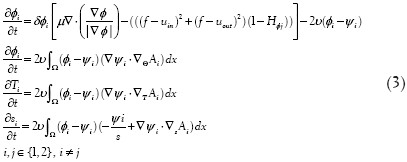
where ψ₁ is defined in Ref.[3]. Similar to the Chan-Vese model, we update u_in and u_out for each iteration as follows:

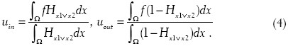
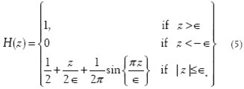
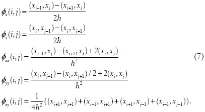
The above model can be adapted for N objects (proof shown in Ref.[3]). The solution to the equations in Equation (4) first requires discretization on a regular two-dimensional M-by-N grid. We let h denote the spacing between the cells and (x₁, y₁) = (i_h, j_h) be the grid points with 0 ≤ i ≥M and 0 ≤ j ≤ N. Discretizing u_in and u_out is straightforward, as long as we fix a regularized Heaviside function. For our discretization we have chosen

To discretize (i.e., divergence of the normalized gradient of φ), we let φ_x, φ_y denote partial derivatives of φ and similarly let φ_xx, φ_yy and φ_xy denote the second-order partial derivatives. Thus, we obtain

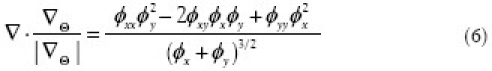
which we discretize with simple finite central differences:

Sequential Algorithm and Implementation

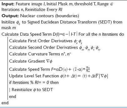
The iterative evolution of the level set φ is described in algorithm 1 using the individual components defined in section 3.2. We start by initializing φ with some initial contour (an ellipse) and set n=0. We then compute u_in (φⁿ) and u_out (φⁿ) from Equation (4). For computing curvature forces, n⁺, n^-, we direct the reader to the formulation.[11] Next we compute Equation (3) with the given discretization above to obtain with explicit forward Euler. Finally, we update n=n+1. Note that we initialize the distance function every RI^th (user defined parameter) iteration.

Algorithm 1.

Sequential level set segmentation

GPU IMPLEMENTATION OF INTEGRATED SHAPE-BASED ACTIVE CONTOUR SCHEME

The GPU-based implementation of the segmentation scheme (described in section 3) is performed with the NVIDIA CUDA toolkit.

Parallel Algorithm and Implementation

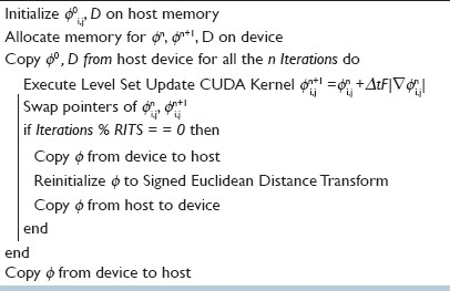
The parallel implementation of the segmentation scheme follows the structure shown in algorithm 2. Input image, I, and an initial contour φ (an ellipse) are both discretized and generated on equally sized 2D grids on CPU. We copy both the image and φ onto the GPU. From this point on, the GPU has everything it needs and requires no further copying of data, thus effectively optimizing memory transfers between the CPU and GPU.

Algorithm 2.

Parallel Implementation

Kernel Threads Setup

In CUDA, it is assumed that both the host (CPU) and device maintain their own DRAM.[8] Host memory is allocated using malloc and device memory is allocated using cudaMalloc. Since memory bandwidth between the host memory and device memory is low (it is much lower than the bandwidth between the device and the device memory), it is recommended to keep the number of transfers to a minimum. In order to minimize the latency of accessing the shared memory it is recommended to make the block size a multiple of 16 and use the cudaMallocPitch routine to allocate memory with padding if the X dimension of the image is not a multiple of 16. Hence, most CUDA programs follow a standard structure of (1) initialization, (2) host to device data transfer, (3) performing computations, and (4) finally memory transfer of computed results from device to host.

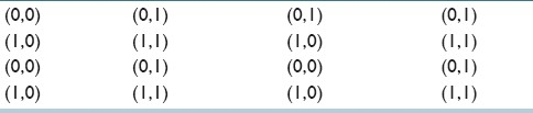
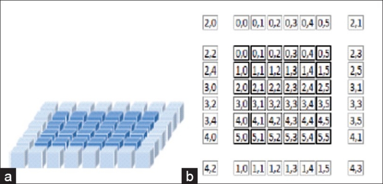
CUDA threads are assigned a unique thread ID that identifies its location within the thread block and grid. This provides a natural way to invoke computation across the image and level set domain, by using the thread IDs for addressing. This is best explained with Table 1. Assume that our image has dimensions 4 × 4 and the block size is 2 × 2. Invoking the kernel with a grid size of 2 × 2 blocks results in the 16 threads shown in Table 1, in the form (threadIdx.y,threadIdx.x). These threads are grouped into blocks of four.

Table 1.

Sample arrangement of 16 threads grouped into blocks of 4

As each thread has access to its ownthreadIdx and blockIdx, global indices (i, j) can be determined using the equations,

int i = blockIdx.x * blockDim.x + threadIdx.x;      (8)

int j = blockIdx.y * blockDim.y + threadIdx.y;

where blockDim.x and blockDim.y represent the dimensions of the block (which in this case are both equal to 2). Of course, much larger block sizes are used, keeping the block X dimension (BX) a multiple of 16 for maximum speed. The effect of different block sizes on performance is analyzed in section 5.5. Once these indices are set up, it is relatively straightforward to transfer the level set update code to a CUDA kernel.

2D Shared Memory Optimization

Since we use finite differences to compute the curvature force in a grid cell, we need to access the value of φ from the neighboring cells (blocks). Unfortunately the GPU is not optimized for this sort of memory access pattern, and memory accesses can suffer a significant performance penalty.[8] In order to keep the number of costly accesses to device memory at a minimum, effective use of the on-chip shared memory is essential. This along with maximizing parallel execution and optimization of instruction usage form the three main performance optimization strategies for CUDA.[8]

Integrating use of the shared memory into the CUDA kernel requires partitioning the level set domain into tiles. For first-order finite difference problems such as ours, each tile must also contain values for neighbor nodes (often known as halo nodes) for i+1 and j+1 elements, which would be stored in separate tiles, so these must also be read into shared memory. As the size of the shared memory is only 16 KB, the sizes of the tiles and corresponding halo are limited. Micikevicius[12] outlined a framework for handling such a process. While such a process may serve as a good model for a multi-GPU implementation, the kernel will need to be modified as it is optimized for higher order stencils (without cross-derivative terms). Instead, tiling code was adapted from Giles’ Jacobi iteration for Laplace discretization algorithm[13] which supports cross-derivatives well. The shared memory management technique in this finite difference algorithm accelerated the global memory implementation by over an order of magnitude.

For a block (and tile) size of BX×BY there are 2×(BX+BY+2) halo elements, as can be seen in Figure 3 where darker elements represent the thread block (the active tile) and the lighter elements represent the halo. It is in this manner that the domain of the computation is partitioned and results in overlapping of halo nodes.

Figure 3.

(a) 2D shared memory arrangement; (b) tile and halo showing a block mapping of thread IDs to halo nodes

Each thread loads φ_n values from global memory to the active tile stored in shared memory. However, depending on the location of the thread within the thread block it may also load a single halo node into the shared memory. Therefore in order to load all halo nodes, this technique assumes that there are at least as many interior nodes as there are halo nodes. Before data can be loaded into the halos, the thread ID needs to be mapped to the location of a halo node both within the halo and within the global indices.

The first 2×(BX+BY+2) threads are assigned to load values into the halo in this manner. This is best visualized with the example of a 6 × 6 thread block as shown in Figure 3b. This method of loading elements has been chosen in order to maximize coalescence, the merging of adjacent blocks of memory to fill gaps caused by deallocated memory. Not only are the interior tile nodes loaded coalesced, but as can be seen above, the first 12 elements of the thread block load the y halos (above and below the interior tile excluding corners) in a coalesced manner. The side halos (x halos) loads are noncoalesced. When writing back results to global memory, as only the interior nodes have updated values they are written to global memory coalesced.

Calculation of Forces

To compute u_in and u_out, we start by computing the value of u_in and u_out in each grid cell, storing it in a temporary array. Since these are scalars values, we use reduction operation,[1] cutting the time spent to O (log n) time assuming we have an infinite number of threads. In a reduction, a binary function is performed on all elements in an array; this can be done in a tree-like fashion, where the given operation can be performed concurrently on different parts of the array and allows for combining the results at the end. NVIDIA has created an STL-like C++ library called thrust that, among other things, can do reductions efficiently on the GPU.

Hereafter, we use the values for u₁ and u₂ computed above to compute the image forces. By image forces, we mean the terms λ₁(f-u₁)² + λ₂(f-u₂)² and the F_shape from Equations (3) and (4). This is straightforward and coalesced (reader is referred to CUDA guide).[9] Lastly, we need to update φ for the next iteration, which is straightforward since we have the two grids containing the curvature force and the image forces. The final step is to copy the new φ back to the CPU.

EXPERIMENTAL RESULTS AND DISCUSSION

Model Parameters, Implementation, and Initialization

In this paper, for the shape model, we generate a training set of 30 ellipses (nuclei and lymphocytes being elliptical in shape) by changing the size of a principal axis with a Gaussian probability function. The manner of choosing the weighting parameters from Equations (1) and (4) is as follows: λ₁=1, λ₂=2, and μ=0.2 determine the size of the neighborhood where the gray value information is averaged by means of diffusion, β_r and β_s are chosen such that the shape prior is attracted toward the region to be segmented. Level sets are manually initialized and the model assumes that the level sets are strategically placed in the vicinity of the objects. Some features such as the Courant--Friedrichs-Lewy (CFL) condition could not be implemented in this parallel version without slowing down computation time significantly.[6] This is because such a condition requires the determination of the largest element of ∇φ which is computed roughly half way through the update procedure. Therefore integrating this condition would require transferring ∇φ and curvature terms back to host memory to determine max {F|∇φ|}, or perhaps more efficiently calling a CUDA kernel to determine the largest element. The cost of this added complexity and slowdown outweighed the benefits, and therefore ∇t was chosen to be a fixed parameter.

All hardware testing was done on a single PC with an Intel Core 2 Duo T8100 Processor with a clock speed of 2.1 GHz and 4 GB of RAM. The graphics hardware used was the NVIDIA GeForce 8600M GT, with CUDA 2.2 software installed. Timing code used was from the cutil library provided in the CUDA toolkit.

Data Description

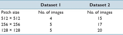
Evaluation is done on two different histopathology datasets: prostate cancer and breast cancer cohorts comprising 14 and 52 images respectively [Table 2]. A total of 70 cancer nuclei from 14 images for prostate and 504 lymphocytes from 52 images for breast cancer were manually delineated by an expert pathologist (serving as the ground truth annotation for quantitative evaluation). For both datasets the objective was to detect, segment the individual nuclei and lymphocytes, and where appropriate, resolve the overlap between intersecting objects. To evaluate the speedup, various patch sizes were created from each of the data set [Table 3].

Table 2.

Description of the different data sets considered in this study

Table 3.

Description of patch sizes from two data sets for which M^GPU and speedup was evaluated

Evaluation of Segmentation and Detection Accuracy

Results shown in Figure 4 for nuclei segmentation aim to demonstrate the strength of our model in terms of detection, segmentation, and overlap resolution accuracy. Table 4 shows the segmentation accuracy (individual lymphocytes and nuclei) compared to those of Chan-Vese[11] (M^CV) and Ali et al.[3] (M^Ali). Note that GPU-based implementation (M^GPU) underperforms in comparison to M^Ali since M^GPU lacks the hybrid boundary based term present in M^Ali. Figure 5 showcases qualitative results of nuclear segmentation achieved by the three models.

Figure 4.

Segmentation results from our model applied to histological image patches of sizes (a), (b) 256×256, (c) 128 × 128 pixels. Note that our model is able to segment intersecting, overlapping nuclei

Table 4.

Quantitative evaluation of segmentation results between models over 66 images

Figure 5.

Segmentation results comparing (a) traditional Chan‐Vese model[11], (b) Ali et al.[3] our GPU-accelerated model

We compute SN, PPV, OR (overlap detection ratio) for each image, and then determine the average and standard deviation across the 62 images. Note that overlap detection ratio 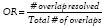is defined as the fraction of total overlaps successfully resolved by the segmentation scheme. These statistics are reported in Table 4 and they reflect the efficacy of M^GPU in segmenting nuclei and lymphocytes in CaP and BC images.

Evaluation of Speedup

We present results of various speedups achieved on data set containing image sizes 256 × 256 and 512 × 512. First we compare the average time taken for 2000 iterations in MATLAB, C, and CUDA on histopathology data of good contrast and dimensions 256 × 256 (a multiple of 16 implying no memory padding is required in CUDA). The results shown in Table 5 reflect the speedup achieved by our GPU-accelerated method.

Table 5.

Comparison of average runtimes for our segmentation algorithm in different programming environments. All comparisons were performed for image patches of size on 256 × 256 and 512 × 512

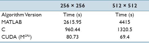
The average runtime speedup attained from sequential code in C to CUDA-optimized code is approximately 13×. The block size used for 2D CUDA compute was 32 × 8. In another experiment, we selected a set of images with relatively poor contrast and dimensions 512 × 512. This makes the image both a computationally demanding segmentation (as it has relatively large dimensions) and challenging in terms of accuracy. The average performance speedup attained on this larger image set was 19×, greater than the speedup attained for the smaller 256 × 256 images. This motivates exploration into the effect of different image sizes on CUDA speedup, discussed in the next section.

Evaluation of the Effects of Image Size on Speedup

Figure 6 shows the effect of multiple patch sizes on computational time for up to 1000 iterations on the optimized CUDA algorithm. It can be seen from Figure 6 that the speedup for smaller sized image patches is relatively less compared to the speedup obtained for images with larger sizes. The sequential algorithm performs almost half as slowly for volume sizes larger than 64². This is most likely due to the fast on board CPU cache being used for smaller volume sizes (<64²) volume sizes larger cannot fit on the CPU cache and hence are stored on the slower DRAM. Conversely, the CUDA code performs relatively poorly for smaller image sizes and much more quickly for larger images. This is essentially due to low numbers of processors being used for such small images and many more being used for larger images. Therefore the speedup line essentially shows that the algorithm follows Amdahl's and Gustafson's laws of parallel computation.[4]

Figure 6.

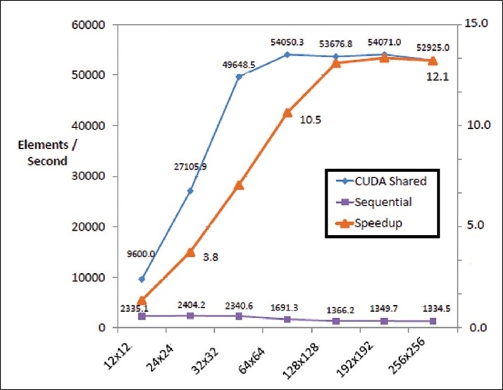
Number of elements computed per second for different volume sizes

Image sizes much larger than 256² could not be tested as the maximum amount of global memory available for the 8600M GT is 256 MB. For example, an 320² image would take up 320²×size of (float) and there are three of these arrays (for the image, previous level set iteration and current level set iteration), which would take up 295 MB of graphics memory. It is however expected, for these even larger volumes, that the speedup of the algorithm will remain at the observed plateau [Figure 6].

CONCLUSIONS

We presented a novel GPU accelerated segmentation scheme that can detect and segment multiple overlapping objects in an image. Our implementation was able to significantly reduce the computational time required for the popular segmentation models, including an integrated active contour scheme with shape priors, inspired by Ali et al.[3] In future work, we intend to extend the framework to incorporate automated model initialization and to evaluate the model on larger image sizes. To further improve the segmentation results, we plan to incorporate a hybrid boundary and region based model with Courant-Friedrichs-Lewy (CFL) condition without compromising the speedup.

Computationally inexpensive segmentation schemes that can accurately segment structures on digitized histology images, especially the ability to deal with overlapping and occluded structures, are highly critical in the context of a number of different diagnostic and prognostic applications. We applied our parallelized algorithm for segmentation and detection of lymphocytes and nuclei in breast and prostate histopathology imagery. We evaluated our algorithm against two popular platforms and with varying image sizes. Our results show that our GPU-accelerated framework was able to segment nuclei and lymphocytes with a speedup of 19×.

REFERENCES

- 1.Madabhushi A. Digital pathology image analysis: Opportunities and challenges (editorial) Imag Med. 2009;1:7–10. doi: 10.2217/IIM.09.9. [DOI] [PMC free article] [PubMed] [Google Scholar]
- 2.Basavanhally A, Ganesan S, Agner S, Monaco J, Feldman M, Tomaszewski J, et al. “Computerized Image-Based Detection and Grading of Lymphocytic Infiltration in HER2+ Breast Cancer Histopathology,”. IEEE Trans Biomed Eng. 2010;57:642–53. doi: 10.1109/TBME.2009.2035305. [DOI] [PubMed] [Google Scholar]
- 3.Ali S, Madabhushi A. “Active Contour For Overlap Resolution Using Watershed Based Initialization (ACOReW): Applications To Histopathology”.IEEE Int Symp Biomed Imag: From Nano to Macro. 2011:614–7. [Google Scholar]
- 4.Kilgariff E, Fernando R. Boston: Addison Wesley; 2005. GPU Gems 2, ch.The GeForce 6 Series GPU Architecture; p. 471491. [Google Scholar]
- 5.Ruiz A, Kong J, Ujaldon M, Boyer KL, Saltz JH, Gurcan MN. “Pathological image segmentation for neuroblastoma using the GPU”.Biomedical Imaging: From Nano to Macro. IEEE International Symposium on. 2008 [Google Scholar]
- 6.Lefohn AE, Whitaker R. “GPU based, three-dimensional level set solver with curvature flow”, technical report uucs-02-017, School of Computing, University of Utah. 2002 [Google Scholar]
- 7.Ali S, Madabhushi A. “Segmenting multiple overlapping objects via an integrated region and boundary based active contour incorporating shape priors: Applications to histopathology”. SPIE Med Imag 79622W. 2011 [Google Scholar]
- 8.NVIDIA CUDA Programming Guide ver 2.2.1. [Accessed May 2011]. Available from: http://www.nvidia.com/object/cuda-develop.html .
- 9.Schmid J, Guitin I, Jos, Gobbetti E, Magnenat-Thalmann N. “A GPU framework for parallel segmentation of volumetric images using discrete deformable model”. Vis Comput. 2011;27:85–95. [Google Scholar]
- 10.Tejada E, Ertl T. “Large steps in GPU-based deformable bodies simulation. Simulat Model Pract Theory. 2005;13:703715. [Google Scholar]
- 11.Chan TF, Vese LA. “Active contours without edges”, IEEE Trans. on Image Process. 2001;10:266–77. doi: 10.1109/83.902291. [DOI] [PubMed] [Google Scholar]
- 12.Micikevicius P. New York, NY, USA: 2009. “3D Fnite difference computation on GPUs using CUDA”, In GPGPU-2: Proceedings of 2nd Workshop on General Purpose Processing on Graph Processing Units, ACM; pp. 79–84. [Google Scholar]
- 13.Giles M. Jacobi iteration for a laplace discretisation on a 3rd structured grid. 2008. Available at people.maths.ox.ac.uk/gilesm/cuda/prac3/laplace3d.pdf .