Bias correction for estimated QTL effects using the penalized maximum likelihood method

Abstract

A penalized maximum likelihood method has been proposed as an important approach to the detection of epistatic quantitative trait loci (QTL). However, this approach is not optimal in two special situations: (1) closely linked QTL with effects in opposite directions and (2) small-effect QTL, because the method produces downwardly biased estimates of QTL effects. The present study aims to correct the bias by using correction coefficients and shifting from the use of a uniform prior on the variance parameter of a QTL effect to that of a scaled inverse chi-square prior. The results of Monte Carlo simulation experiments show that the improved method increases the power from 25 to 88% in the detection of two closely linked QTL of equal size in opposite directions and from 60 to 80% in the identification of QTL with small effects (0.5% of the total phenotypic variance). We used the improved method to detect QTL responsible for the barley kernel weight trait using 145 doubled haploid lines developed in the North American Barley Genome Mapping Project. Application of the proposed method to other shrinkage estimation of QTL effects is discussed.

Introduction

Epistasis, the interaction between genes, is an important process in genetics, selection and evolution (Lynch and Walsh, 1998; Carlborg and Haley, 2004; Melchinger et al., 2007), and use of the epistatic genetic model has been popular in genetic dissection of complex traits (Cheverud and Routman, 1995; Carlborg and Haley, 2004; Zhang and Xu, 2005; Melchinger et al., 2007; He and Zhang, 2008). However, the model dimension increases quickly as the number of loci increases. The number of parameters is often larger than the sample size, producing what is known as an oversaturated model. In this situation, the most commonly used least squares and maximum likelihood methods are not feasible.

Recently, statistical methods have been proposed to handle such oversaturated model. In general, there are two approaches: variable selection (Akaike, 1973; Hocking, 1976; Schwarz, 1978; Ball, 2001; Broman and Speed, 2002) and shrinkage estimation (Hoerl and Kennard, 1970; Tibshirani, 1996; Xu, 2003, 2007a; Zhang and Xu, 2005). For variable selection, stepwise regression that progressively adds or deletes a quantitative trait locus (QTL) as well as an epistatic effect in the model (Moreno-Gonzalez, 1993) is one of the most important methods. For the shrinkage estimation, ridge regression (Hoerl and Kennard, 1970; Whittaker et al., 2000; Boer et al., 2002) is not a viable choice for QTL mapping if the model includes all markers of the entire genome. The reason for this is that the estimation treats all effects equally across loci (Xu, 2003). In the stochastic search variable selection of George and McCulloch (1993) and Yi et al. (2003), effects included in the model have one common prior variance, and effects excluded from the model have another common prior variance. However, the two prior variances are artificially determined. To overcome this issue, the Bayesian shrinkage estimation method was developed (Meuwissen et al., 2001; Xu, 2003; Wang et al., 2005). In this method, each effect is assigned a normal prior distribution with a mean of zero and a unique variance. The effect-specific prior variance is further assigned a vague prior such that the variance can be estimated from the data. Although this method has been validated by rigorous statistical proof, it is an Markov chain Monte Carlo implemented approach and thus is computationally demanding. In addition, the least absolute shrinkage and selection operator (LASSO) is commonly used (Tibshirani, 1996; Scott, 2007), but this method is difficult to implement and often has a high false positive rate in the detection of QTL, which will be demonstrated in a later section of this study. To save computing time, Zhang and Xu (2005) incorporated the idea of Bayesian shrinkage estimation into the maximum likelihood method. This method, called penalized maximum likelihood (PML), adopts a penalty that depends on the values of the parameters. It allows spurious QTL effects to be shrunk towards zero, while QTL with large effects is estimated with virtually no shrinkage. The main advantages of this approach over other methods are reflected by its simplicity and fast speed.

Zhang and Xu (2005) used the PML method to estimate epistatic effects of an oversaturated genetic model. However, the PML method is not optimal in two special cases: (1) closely linked QTL with effects in opposite directions and (2) small-effect QTL. The reason for this is that the method shrinks true small effects and spurious effects in the same way and causes all effects (true and false) to bias downwardly. In theory, shrinkage estimation refers to the biased estimation of a regression coefficient towards zero using a prior variance as a factor to control the degree of shrinkage (Xu, 2007b). To overcome the above shortcomings of the PML method, we should correct the bias in the estimation of QTL effects. As for the correction, Guo (2007) used the PML method to select QTL and employed the least squares method to estimate the effects of the selected QTL, and Luo et al. (2003) used the variance of estimate to correct the genetic variance of each individual QTL. In this study, we consider an alternative approach.

Under the Bayesian framework, a QTL effect is generally assigned a normal prior. The variance parameter in the normal prior is further assigned a uniform prior (Zhang and Xu, 2005), the Jeffreys prior (Wang et al., 2005) or a scaled inverse chi-square prior (Chen et al., 2010). The first two priors are special cases of the scaled inverse chi-square prior (Xu, 2010). In Zhang and Xu (2005), we adopted the uniform prior for the variance parameter. In this study, we substitute the uniform prior with a more general scaled inverse chi-square prior. We demonstrate that these modifications are able to correct the bias and improve the power of QTL detection.

Theory and methods

Genetic model

Let y_i (i=1, 2, …, n) be the phenotypic value of the ith individual in a backcross population of sample size n. The genetic model under consideration is

where b₀ is the population mean, x_il is a dummy variable indicating the genotype of the lth marker for individual i, b_l is the effect of marker l (l=1, 2, …, q), q is the total number of markers on the entire genome, b_rs is the epistatic effect between markers r and s, and ɛ_i is the residual error with an assumed N(0,σ²) distribution. The dummy variable is defined as x_il=1 for heterozygote and x_il=−1 for homozygote for a backcross individual.

For clarity of notation, we use j to index the jth genetic effect, including the additive and epistatic effects. Model (1) is then rewritten as

where x_ij=x_il and b_j=b_l if the jth effect is a main effect, x_ij=x_irx_is and b_j=b_rs if the jth effect is an epistatic effect and p=q(q+1)/2. Now, we have a simple model that includes both the main and the epistatic effects.

Prior distribution

In the PML method of Zhang and Xu (2005), the penalty is a function of the parameters, and the prior density of the parameters in the Bayesian framework is an ideal choice for the penalty factor. The prior distributions in Zhang and Xu (2005) are briefly described below. The parameters b₀ and σ² are always included in the model; therefore, their inclusion should not be penalized. We adopt the normal prior for each of the genetic effects (b_j) in model (2),

where φ(b_j; μ_j,σ_j²) is the normal density with mean μ_j and variance σ_j². The normal and uniform priors are further assigned to μ_j and σ_j², respectively,

where η=5 (Zhang and Xu, 2005). We replace the uniform prior with a scaled inverse chi-square prior, of which the uniform prior is a special case (Xu, 2010):

Monte Carlo simulation studies showed that (τ, ω)=(−3.5, 0) is the best choice for the set of hyperparameters because a higher power of QTL detection and lower mean squared error (MSE) were achieved (Supplementary Figure S1). Some theoretical considerations of our method are given in Appendix A.

Bias correction

Define θ={b₀, b_1, …, b_p, σ²} and ξ={μ₁, …, μ_p, σ₁², …, σ_p²}. The parameters are estimated by maximising the penalized log likelihood function

with respect to θ and ξ simultaneously, where

and

To correct the bias of the estimated QTL effect, P(θ,ξ) is replaced by

where k_j is a bias correction coefficient. We will describe how to determine the most suitable k_j value in Result. Therefore, the PML function is set to

The PML estimate of the intercept is found by setting

and solving for b₀, which is

Setting

and solving for b_j (j=1, …, p), we obtain

If σ_j² → 0, then b_j → μ_j. Additionally, , so b_j → 0. This explains why the estimate of a false QTL effect is close to zero. If σ_j² is far away from zero, k_j can be used to adjust the estimate of b_j, and a suitable k_j value is used to obtain an unbiased estimate of b_j.

The residual error variance is estimated by setting

and solving for σ², which is

The PML estimates of the nuisance parameters are

The iterative steps in the estimation of parameters are identical to those given by Zhang and Xu (2005). The criterion of convergence is

In this study, we considered two new methods: (1) the method with k_j≠1 (bias correction only) and (2) the method with k_j≠1 and τ≠−2 (bias correction and different level of shrinkage), which are abbreviated as bias-correction PML (BPML) and bias-correction and shrinkage PML (BSPML), respectively.

Likelihood ratio test

As stated by Zhang and Xu (2005), the usual likelihood ratio test (LRT) cannot be carried out with the PML method because the model is oversaturated. We proposed the following two-stage selection process to scan the markers (Zhang and Xu, 2005). In the first stage, all effects with are chosen. In the second stage, the full model is modified such that only the markers that pass the first round of selection are included in the model. Thanks to the smaller dimension of the reduced model, we can use the maximum likelihood method to re-analyse the data and perform the LRT.

The procedure for calculating the LRT statistic is the same as that used in Zhang and Xu (2005). Let s be the total number of QTL effects that have passed the first round of selection and θ′={b₀, b₍₁₎, …, b_(s), σ²} be the parameters that are subject to the maximum likelihood analysis for the significance test. To test the null hypothesis that H₀:b_(j)=0, that is, the jth surviving QTL is not true, we use the following LRT statistic,

where θ′_−j={b₀, b₍₁₎, …, b_(j−1), b_(j+1), …, b_(s), σ²} is the vector of parameters that excludes b_(j) (1, …, s). As pointed out by Kao et al. (1999), the choice of the critical value for claiming a significant QTL becomes complex for multiple QTL test. For simplicity, we use logarithm of odds (LOD)⩾2.0 as the criterion (Lander and Kruglyak, 1995; Qin et al., 2008; He et al., 2011) for the simulated data and the usual LOD⩾2.5 (He et al., 2011) as the criterion for real data analysis, where LOD=LR/ln(10).

Results

Monte Carlo simulation studies

The purpose of the simulation studies was to demonstrate that (1) the BPML method is more efficient than the PML method and the BSPML method is better than the BPML method and (2) the BSPML method is as efficient as the currently adopted methods, such as the empirical Bayes (eBayes) method (Xu, 2007a).

We simulated a backcross population using a sample size of 600. Two hundred forty-one evenly spaced markers were simulated on one chromosome segment of 2400 cM in length. A total of 20 QTL were simulated, all of which were placed at marker positions. The sizes and locations of the QTL are listed in Table 1. These parameters were used to generate the phenotypic observations of a quantitative trait with a population mean b₀=100 and a residual error variance σ²=10.0. We generated a total of 500 data sets (replications) from the same parameter setup. Each of the 500 simulated data sets was analysed by the PML, BPML, BSPML, eBayes and LASSO approaches (Xu, 2010). For each simulated QTL, we counted the samples in which the LOD statistic exceeded 2.0. A detected QTL within 20 cM of the simulated QTL was considered a true QTL. The ratio of the number m of such samples to the total number of replicates (500) represented the empirical power of this QTL. The false positive rate was calculated as the ratio of the number of false positive effects to the total number of zero effects considered in the full model. We used the MSE of estimated QTL effects to further evaluate the performance of the extended methods. The MSE for the jth QTL is defined as , where is the estimate of b_j in the ith sample.

Table 1. Effects and positions of the simulated quantitative trait loci (QTL).

QTL	True value			QTL	True value
	Position (cM)	Effect	r2(%)		Position (cM)	Effect	r2(%)
1	50	4.47	19.29	11	910	3.81	15.02
2	120	3.16	9.64	12	920	2.25	4.89
3	210	−2.24	4.85	13	1100	−1.30	1.63
4	240	−1.58	2.41	14	1210	−1.00	0.97
5	350	2.24	4.85	15	1300	−2.24	4.85
6	360	3.16	9.64	16	1340	1.58	2.41
7	610	1.10	1.17	17	1350	1.00	0.97
8	630	−1.10	1.17	18	1370	−1.73	2.89
9	800	0.77	0.57	19	1800	0.71	0.49
10	900	1.73	2.89	20	2300	0.89	0.76

To select a suitable k_j value in the BPML and BSPML approaches, each of the 500 simulated data sets was analysed by varying k_j from 0.2 to 1.2 incremented by 0.2. The most suitable k_j value was determined by high power of QTL detection, low MSE and small bias of the estimated QTL effect. For example, the highest power, the lowest MSE and the least bias for the 7th and 8th QTL are always achieved using k_j=0.2 (Supplementary Figure S2). This finding means that k_j should be set to 0.2 for the 7th and 8th QTL.

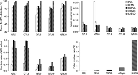
To achieve the first objective of the simulation experiment, each of the 500 simulated data sets was analysed by the PML, BPML and BSPML approaches. The results are shown in Figure 1. Compared with the PML method, the BPML method increased the power of detection for the 7th and 8th QTL (closely linked QTL) from 23 to 85%, decreased the MSE from 0.260 to 0.085, and reduced the standard deviations of the positions and the effects for the simulated QTL. The same trend was also observed for the 17th QTL (closely linked to the 16th QTL with the same sign) (data not shown). Compared with the PML method, the BPML method increased the power of detection of the 19th QTL (small-effect QTL) from 56.0 to 84.8% and decreased the standard deviation of the position and the effect for the 19th QTL. When we further replaced the uniform prior of the variance parameter by the scaled inverse chi-square prior, a further improvement in QTL detection was achieved. For example, the power of the detection of the 17th QTL increased from 37.4 to 60.2% and the MSE decreased from 0.275 to 0.059. Therefore, the BSPML method is the best of the three aforementioned methods.

Figure 1.

Results of QTL mapping from the simulated data sets (500 replicates) using the PML, BPML, BSPML, eBayes and LASSO methods. Note that the true effect values for the 7th, 8th, 9th, 19th and 20th QTL are 1.1, −1.1, 0.77, 0.71 and 0.89, respectively.

To achieve the second objective of the simulation experiment, each of the 500 simulated data sets was analysed by the BSPML, eBayes and LASSO approaches. The results are shown in Figure 1. Based on the power of QTL detection, the MSE and the standard deviations of the estimated positions and the effects of QTL, the LASSO method is the best of the three methods, and the BSPML method is as efficient as the eBayes method. However, the LASSO method has the highest false positive rate, whereas the others have low false positive rates.

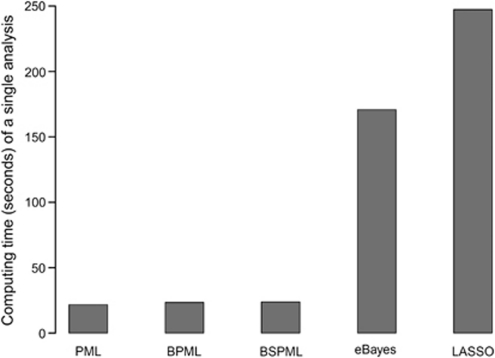
The computing times for completing a single data analysis using the previously described methods, implemented by the SAS program, are also given in Figure 2. The results show that the BSPML method is faster than the other methods.

Figure 2.

Computing time (in s) of a single analysis from a backcross population of 600 lines using various approaches, implemented by the SAS program, on a Pentium PC with 2.80 GHz processor and 2.00 GB RAM.

Real data analysis in barley

The well-known barley data set from the North American Barley Genome Mapping Project (Tinker et al., 1996) was used for the demonstration. The data set was collected from a doubled haploid population that contained 145 lines, each of which was grown in 25 different environments. The phenotype analysed was the average value of the kernel weight across environments. A total of 127 markers covering a genome of 1500 cM (seven linkage groups) were used in the analysis. Xu (2007a) re-analysed this data set using eBayes and LASSO. A total of six main-effect QTL were identified on five linkage groups. The sizes of the identified QTL ranged from 1.01 to 30.30% of the phenotypic variance (Tinker et al., 1996; Xu, 2007a). The overall contribution of the six QTL to the phenotypic variance was from 28.70 to 62.18% across various methods.

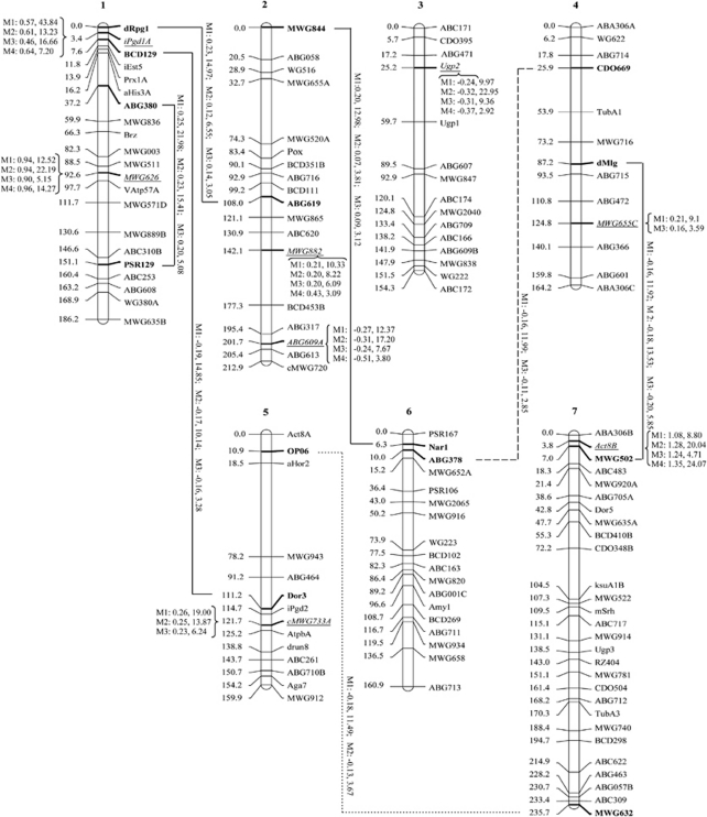
This data set was re-analysed in this study. Due to incomplete marker genotypic information and unevenly distributed marker density, the procedure requires a pre-treatment. When the marker density is high, choosing one marker from a cluster of highly linked markers can avoid a high degree of multicollinearity. When the marker density is too sparse (>5 cM), a virtual marker (treated as missing data) may be inserted (Xu et al., 2011). In the case of incomplete marker information, marker imputation techniques can be used. Usually, 30–50 imputed data sets are generated. In this study, we imputed 100 samples for the missing genotypes using the conditional probability of incomplete marker genotypes calculated by the multipoint method (Rao and Xu, 1998). This approach requires multiple analyses of the data sets; each of the 100 imputed data sets was analysed by the BSPML, eBayes and LASSO methods. The total number of QTL effects included in the model was q(q+1)/2, where q=127. The number of effects was ∼56 times the sample size. In other words, the model was overloaded. In this case, a two-stage method was proposed. In the first stage, the full model including all the main and pairwise epistatic effects was divided into many reduced models. Each reduced model contained all the main effects and a portion (∼500) of the epistatic effects. It was feasible to estimate the parameters of each reduced model. In the second stage, we modified our epistatic genetic model such that only effects that have passed the first round of selection were included in the model, and re-analysed the data under the modified genetic model using the BSPML, eBayes and LASSO methods. The critical value of LOD score for declaration of significance was set to 2.5. For the BSPML method, we needed to select a suitable value for k_j. Therefore, each of the 100 imputed data sets was analysed by setting k_j at 0.2, 1.0 and 1.2. A suitable k_j value was determined as the one that produced the highest ratio of the number of QTL detected to the total number of imputed data sets. If the ratio ties, then the k_j value with the largest LOD value is recommended. This is because the MSE and the bias of QTL effect estimates cannot be calculated when the true value of the parameter is unknown. The results are listed in Supplementary Tables S1 and S2. From the two tables, we were able to determine the most suitable k_j value. In addition, the original data set was also analysed using composite interval mapping (Wang et al., 2007), and its critical LOD score was calculated by performing 1000 permutation experiments. The results are shown in Figure 3. As a result, eight main-effect QTL and seven epistatic QTL were detected. The seven main-effect QTL that were originally identified by the eBayes in Xu (2007a) were all detected by the BSPML method. The additional main-effect QTL mapped in the analysis was confirmed by the LASSO method, suggesting that the BSPML is more powerful. Results of all the methods showed that main effects are more important than epistatic effects (Xu, 2007a), because the main effects collectively explain 55.1% of the total phenotypic variation of the trait. The corresponding proportions obtained from the eBayes, LASSO and composite interval mapping analyses are 77.1, 75.3 and 75.8%, respectively.

Figure 3.

The locations and effects of QTL detected with the BSPML (M1), eBayes (M2), LASSO (M3) and composite interval mapping (M4) methods. The effects and LOD scores for the detected QTL are also given in the figure. For the main-effect QTL, effects and LOD scores are placed at the positions of the detected QTL. For the epistatic QTL, the effects and LOD scores are placed along with the lines that connect the interacting loci. Solid lines indicate that the interactions were detected by all three methods. Dotted lines indicate that the interactions were detected by only two methods.

Cross-validation

The entire barley data set was split into five subsets, each with 29 lines. The training data consisted of four subsets for parameter estimation and the testing data consisted of the remaining data set for the evaluation of the predicted error of the kernel weight. Each of the five subsets was treated as a testing data set in turn and eventually the kernel weights of all lines were predicted. The mean prediction error (MPE), defined below, was used as a measurement of the efficiency of a method,

A smaller MPE indicates a higher efficiency for a method. The second index of the efficiency is the R² value, defined as

where is the phenotypic variance of the trait. The final measurement is the Pearson's correlation coefficient squared (r²) between the observed phenotypic value y and the predicted value The five-fold cross-validation was applied to all the four methods (PML, BSPML, eBayes and LASSO) for the barley kernel weight trait. The results are listed in Table 2, from which we can see that the BSPML method is comparable to the eBayes method, although the LASSO method outperformed both methods.

Table 2. Results of cross-validation experiment under the epistatic genetic model for the barley kernel weight trait using the PML, eBayes, BSPML and LASSO methods.

Method	Mean prediction error	R2a	r2b
PML	3.034	0.3557	0.4886
eBayes	2.657	0.4356	0.5075
BSPML	2.269	0.5182	0.5359
LASSO	2.229	0.5265	0.5402

Abbreviations: BSPML, bias-correction and shrinkage penalized maximum likelihood; LASSO, least absolute shrinkage and selection operator; MPE, mean prediction error; PML, penalized maximum likelihood.

^aR²=1−MPE/mean squared deviation, where and

^bPearson's correlation coefficient squared.

Discussion

Bias correction works well in the detection of both small and linked QTL. This conclusion means that the method proposed in this study is efficient in detecting small and closely linked QTL. To further validate the new method, the idea of bias correction in this study was incorporated into both eBayes and LASSO. The two extended methods were also used to analyse the simulated data sets in the Monte Carlo studies. The results show that the extended eBayes method is better than the original eBayes method because a higher power of QTL detection and lower MSE of QTL effect estimate were achieved (Supplementary Figure S3). Moreover, the improvement in the LASSO method was minor (data no shown). In addition, this idea may be incorporated into Bayesian shrinkage analysis, which is expected to yield a similar improvement.

The BSPML method is different from Zhang and Xu's (2005) original method in two aspects. First, the new method corrects the bias in the estimated QTL effect by using tuning parameter. The selected tuning parameters are based on simulations, and thus are valid for the detection of QTL under the assumptions and overall range of effect sizes included in the simulations. The idea is further confirmed by real data analysis in this study. This correction is different from those of the shrinkage interval mapping proposed by Guo (2007) and Luo et al. (2003). For the two special situations in this study, the bias correction increased the power of QTL detection and the precision of the parameters by solving the two problems in Zhang and Xu (2005), as demonstrated in Figure 1. Second, we replaced the uniform prior of the variance parameter of the QTL effect by a more general scaled inverse chi-square prior. As a result, the estimates of b_j and σ_j² in the BSPML method are different from those in the original PML method.

Although the scaled inverse chi-square has been considered as a prior distribution for σ_j² in the PML method of Lü et al. (2009), there are some subtle differences between that method and the one proposed here. The former seeks to decrease the false positive rate in the detection of QTL by increasing the value of τ, whereas the latter seeks to enhance the QTL detection ability by decreasing the value of τ. In this study, we selected a suitable value for τ that maintained a high statistical power and a low false positive rate.

The well-known barley data set has often been used to detect QTL for kernel weight in barley (Tinker et al., 1996; Xu, 2007a). However, the methodologies used in these previous studies differ greatly from the technique used in this study. For example, Tinker et al. (1996) used simplified composite interval mapping to detect main-effect QTL and QTL-by-environment interactions. Among these main-effect QTL, six were further detected in this study. Our results also agree with the previously published results of Xu (2007a) because all the kernel weight loci detected by the eBayes of Xu (2007a) were also identified in this study. All methods indicated that markers Act8B and MWG626 are closely associated with kernel weight. The two markers may be used in marker-assisted selection.

In molecular breeding, identification of small-effect QTL remains a challenging problem because it is difficult to identify and utilise small-effect QTL in marker-assisted breeding. The improved method proposed in this study produced high power, particularly in the detection of closely linked and small-effect QTL. This suggests the feasibility of utilising these QTL in future marker-assisted breeding.

Appendix A

Some theoretical consideration of our method

The hierarchical priors of our method are given below,

The joint distribution for b_j and μ_j is

The marginal distribution of b_j is

Comparing this prior with the zero mean normal prior

we can see that we increased the standard prior variance to a larger prior variance

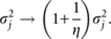This may explain why we can choose τ=−3.5 to composite this large prior variance.

The proof of

is straightforward because we can use the property of normal distribution and the property of variance. Let

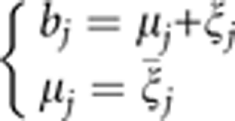where

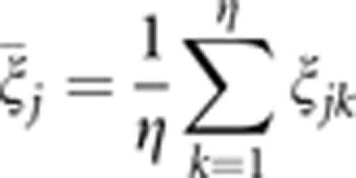is assumed to be the average of η error terms, each of which is sampled from the same distribution N(σ_j²). This was the original idea when we developed the penalized maximum likelihood method. Using

we can show that

The authors declare no conflict of interest.

References

- Akaike H.1973Information theory and an extension of the maximum likelihood principleIn: Petrox BN, Caski F (eds).Second International Symposium on Information Theory Akademiai Kiado: Budapest; 267–281. [Google Scholar]
- Ball RD. Bayesian methods for quantitative trait loci mapping based on model selection: approximate analysis using the Bayesian information criterion. Genetics. 2001;159:1351–1364. doi: 10.1093/genetics/159.3.1351. [DOI] [PMC free article] [PubMed] [Google Scholar]
- Boer MP, Braak CJF, Jansen RC. A penalized likelihood method for mapping epistatic quantitative trait loci with one-dimensional genome searches. Genetics. 2002;162:951–960. doi: 10.1093/genetics/162.2.951. [DOI] [PMC free article] [PubMed] [Google Scholar]
- Broman KW, Speed TP. A model selection approach for the identification of quantitative trait loci in experimental crosses. J R Stat Soc B. 2002;64:641–656. doi: 10.1534/genetics.108.094565. [DOI] [PMC free article] [PubMed] [Google Scholar]
- Carlborg Ö, Haley CS. Epistasis: too often neglected in complex trait studies. Nat Rev Genet. 2004;5:618–625. doi: 10.1038/nrg1407. [DOI] [PubMed] [Google Scholar]
- Chen X, Zhao F, Xu S. Mapping environment specific quantitative trait loci. Genetics. 2010;186:1053–1066. doi: 10.1534/genetics.110.120311. [DOI] [PMC free article] [PubMed] [Google Scholar]
- Cheverud JM, Routman EJ. Epistasis and its contribution to genetic variance components. Genetics. 1995;139:1455–1461. doi: 10.1093/genetics/139.3.1455. [DOI] [PMC free article] [PubMed] [Google Scholar]
- George EI, McCulloch RE. Variable selection via Gibbs sampling. J Am Stat Assoc. 1993;91:883–904. [Google Scholar]
- Guo Z.2007Novel method for increasing efficiency of quantitative trait locus mappingPhD thesis,Kansas State University, Manhattan, Kansas [Google Scholar]
- He XH, Qin HD, Hu ZL, Zhang TZ, Zhang YM. Mapping of epistatic quantitative trait loci in four-way crosses. Theor Appl Genet. 2011;122:33–48. doi: 10.1007/s00122-010-1420-8. [DOI] [PubMed] [Google Scholar]
- He XH, Zhang YM. Mapping epistatic QTL underlying endosperm traits using all markers on the entire genome in random hybridization design. Heredity. 2008;101:39–47. doi: 10.1038/hdy.2008.23. [DOI] [PubMed] [Google Scholar]
- Hocking RR. The analysis and selection of variables in linear regression. Biometrics. 1976;32:1–49. [Google Scholar]
- Hoerl AE, Kennard RW. Ridge regression: biased estimation for nonorthogonal problems. Technometrics. 1970;12:55–67. [Google Scholar]
- Kao CH, Zeng ZB, Teasdale RD. Multiple interval mapping for quantitative trait loci. Genetics. 1999;152:1203–1216. doi: 10.1093/genetics/152.3.1203. [DOI] [PMC free article] [PubMed] [Google Scholar]
- Lander ES, Kruglyak L. Genetic dissection of complex traits guidelines for interpreting and reporting linkage results. Nat Genet. 1995;11:241–247. doi: 10.1038/ng1195-241. [DOI] [PubMed] [Google Scholar]
- Lü HY, Li M, Li GJ, Yao LL, Lin F, Zhang YM. Multiple loci in silico mapping in inbred lines. Heredity. 2009;103:346–354. doi: 10.1038/hdy.2009.66. [DOI] [PubMed] [Google Scholar]
- Luo L, Mao Y, Xu S. Correcting the bias in estimation of genetic variances contributed by individual QTL. Genetica. 2003;119:107–113. doi: 10.1023/a:1026028928003. [DOI] [PubMed] [Google Scholar]
- Lynch M, Walsh JB. Genetics and Analysis of Quantitative Traits. Sinauer Associates: Sunderland, MA; 1998. [Google Scholar]
- Melchinger AE, Utz HF, Piepho HP, Zeng ZB, Schön CC. The role of epistasis in the manifestation of heterosis: a systems-oriented approach. Genetics. 2007;177:1815–1825. doi: 10.1534/genetics.107.077537. [DOI] [PMC free article] [PubMed] [Google Scholar]
- Meuwissen THE, Hayes BJ, Goddard ME. Prediction of total genetic value using genome-wide dense marker maps. Genetics. 2001;157:1819–1829. doi: 10.1093/genetics/157.4.1819. [DOI] [PMC free article] [PubMed] [Google Scholar]
- Moreno-Gonzalez J. Efficiency of generations for estimating marker-associated QTL effects by multiple regression. Genetics. 1993;135:223–231. doi: 10.1093/genetics/135.1.223. [DOI] [PMC free article] [PubMed] [Google Scholar]
- Qin H, Guo W, Zhang Y, Zhang T. QTL mapping of yield and fiber traits based on a four-way cross population in Gossypium hirsutum L. Theor Appl Genet. 2008;117:883–894. doi: 10.1007/s00122-008-0828-x. [DOI] [PubMed] [Google Scholar]
- Rao S, Xu S. Mapping quantitative trait loci for ordered categorical traits in four-way crosses. Heredity. 1998;81:214–224. doi: 10.1046/j.1365-2540.1998.00378.x. [DOI] [PubMed] [Google Scholar]
- Schwarz GE. Estimating the dimension of a model. Anna Stat. 1978;6:461–464. [Google Scholar]
- Scott F.2007The LASSO linear mixed model for mapping quantitative trait lociPhD thesis,The University of Adelaide, Adelaide, SA [Google Scholar]
- Tibshirani R. Regression shrinkage and selection via the LASSO. J R Stat Soc Series (Methodol) 1996;58:267–288. [Google Scholar]
- Tinker NA, Mather DE, Rossnagel BG, Kasha KJ, Kleinhofs A, Hayes P, et al. Regions of the genome that affect agronomic performance in two-row barley. Crop Sci. 1996;36:1053–1062. [Google Scholar]
- Wang H, Zhang YM, Li X, Masinde GL, Mohan S, Baylink DJ, et al. Bayesian shrinkage estimation of QTL parameters. Genetics. 2005;170:465–480. doi: 10.1534/genetics.104.039354. [DOI] [PMC free article] [PubMed] [Google Scholar]
- Wang S, Basten C, Zeng ZB. Windows QTL Cartographer 2.5. Department of Statistics, North Carolina State University: Raleigh, NC; 2007. [Google Scholar]
- Whittaker JC, Thompson R, Denham MC. Marker-assisted selection using ridge regression. Genet Res. 2000;75:249–252. doi: 10.1017/s0016672399004462. [DOI] [PubMed] [Google Scholar]
- Xu S. Estimating polygenic effects using markers of the entire genome. Genetics. 2003;163:789–801. doi: 10.1093/genetics/163.2.789. [DOI] [PMC free article] [PubMed] [Google Scholar]
- Xu S. An empirical Bayes method for estimating epistatic effects of quantitative trait loci. Biometrics. 2007a;63:513–521. doi: 10.1111/j.1541-0420.2006.00711.x. [DOI] [PubMed] [Google Scholar]
- Xu S. Derivation of the shrinkage estimates of quantitative trait locus effects. Genetics. 2007b;177:1255–1258. doi: 10.1534/genetics.107.077487. [DOI] [PMC free article] [PubMed] [Google Scholar]
- Xu S. An expectation–maximization algorithm for the Lasso estimation of quantitative trait locus effects. Heredity. 2010;105:483–494. doi: 10.1038/hdy.2009.180. [DOI] [PubMed] [Google Scholar]
- Xu Y, Li HN, Li GJ, Wang X, Cheng LG, Zhang YM. Mapping quantitative trait loci for seed size traits in soybean (Glycine max L. Merr.) Theor Appl Genet. 2011;122:581–594. doi: 10.1007/s00122-010-1471-x. [DOI] [PubMed] [Google Scholar]
- Yi N, George V, Allison DB. Stochastic search variable selection for identifying quantitative trait loci. Genetics. 2003;164:1129–1138. doi: 10.1093/genetics/164.3.1129. [DOI] [PMC free article] [PubMed] [Google Scholar]
- Zhang YM, Xu S. A penalized maximum likelihood method for estimating epistatic effects of QTL. Heredity. 2005;95:96–104. doi: 10.1038/sj.hdy.6800702. [DOI] [PubMed] [Google Scholar]
Associated Data
This section collects any data citations, data availability statements, or supplementary materials included in this article.