COMPARISON FRICTION: EXPERIMENTAL EVIDENCE FROM MEDICARE DRUG PLANS

Abstract

Consumers need information to compare alternatives for markets to function efficiently. Recognizing this, public policies often pair competition with easy access to comparative information. The implicit assumption is that comparison friction—the wedge between the availability of comparative information and consumers’ use of it—is inconsequential because information is readily available and consumers will access this information and make effective choices. We examine the extent of comparison friction in the market for Medicare Part D prescription drug plans in the United States. In a randomized field experiment, an intervention group received a letter with personalized cost information. That information was readily available for free and widely advertised. However, this additional step—providing the information rather than having consumers actively access it—had an impact. Plan switching was 28 percent in the intervention group, versus 17 percent in the comparison group, and the intervention caused an average decline in predicted consumer cost of about $100 per year among letter recipients—roughly 5 percent of the cost in the comparison group. Our results suggest that comparison friction can be large even when the cost of acquiring information is small, and may be relevant for a wide range of public policies that incorporate consumer choice.

I. Introduction

Government services increasingly rely on consumer choice. For instance, the design of the largest new social program of the last decade, Medicare Part D prescription drug insurance, relies heavily on consumers making choices. Choice is a key feature of Social Security privatizations and proposed school voucher programs. The rationale for including choice and competition is straightforward. Individuals have heterogeneous preferences and choice allows them to opt for services that best match their preferences. Competition between providers then facilitates a menu of services being provided at the cost-efficient frontier. In the best case, consumers get services that fit their needs better and governments save money.

This best case requires that consumers be able to look at the menu of options and pick the one that most cost effectively matches their needs. Making such choices requires having informed consumers. Yet, service providers may not provide all relevant information voluntarily. When service providers have information relevant to choices that consumers do not, this information asymmetry can undercut the benefits of choice and competition. As a result, policymakers frequently pair choice mechanisms with transparency systems—such as public school report cards, nutritional labeling, toxic pollution reporting, auto safety and fuel economy ratings, and corporate financial reporting (Weil et al. 2006)—all intended to make comparative information readily available.

Simply making information available, however, does not ensure consumers will use it. We call comparison friction the wedge between the availability of comparative information and consumers’ use of it. (It is analogous to search friction—the challenge for buyers and sellers in locating each other.) Traditionally, public policies assume that comparison friction is largely inconsequential as long as comparative data is provided for free and the benefits from comparing are non-negligible.

This study estimates the effect of reducing comparison friction in the market for prescription drug insurance plans for senior citizens. Over a period of about two and a half years, we followed the choices made by seniors who participated in an experiment we designed that reduced comparison friction by delivering personalized cost information to seniors via a letter. That personalized information used aspects of the match between consumers and the available plans (specifically, the differences in out-of-pocket costs of the drugs an individual takes) that could be readily observed.

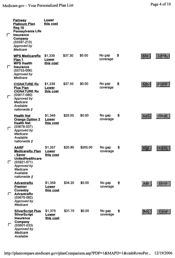
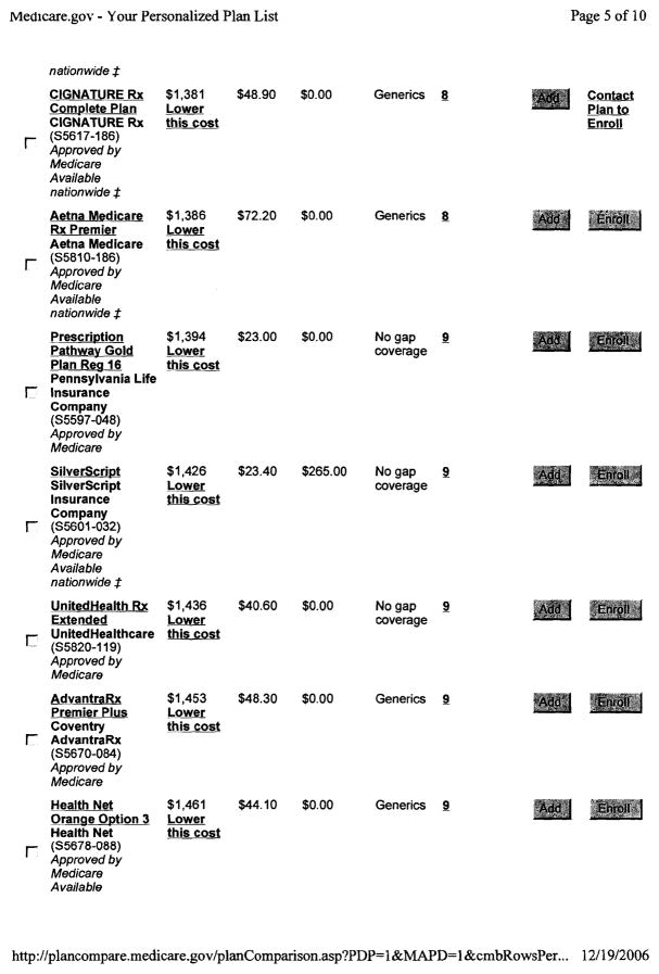
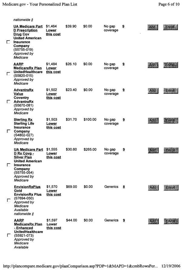
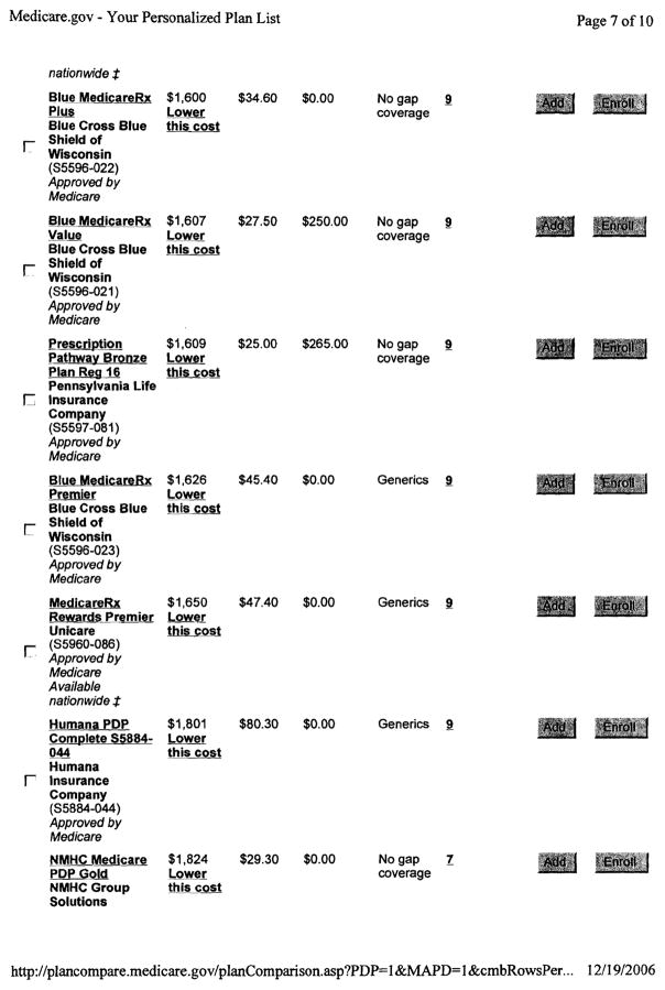
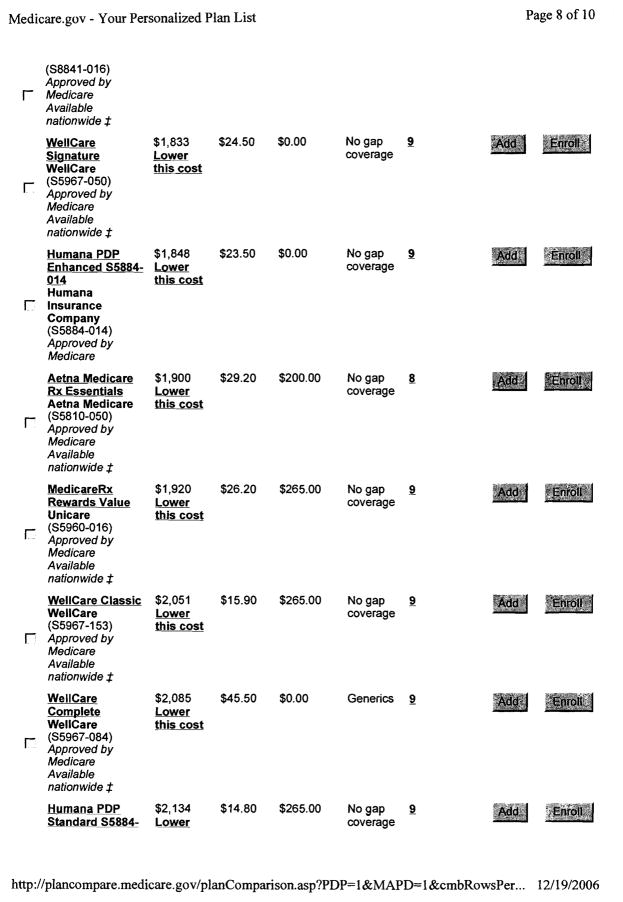
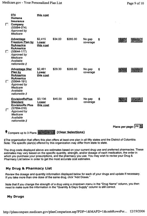
One group of seniors—the intervention group—was presented with personalized price information created by entering their drug data into Medicare’s Plan Finder website. They saw the cost of all plans for their personal drug profile as well as how much they would save by switching to the lowest-cost plan. A comparison group was given only the address of this website. The distinction between the groups was that the comparison group had to actively visit a website (or call Medicare’s toll-free number, or seek information from a third party), whereas the intervention group had information delivered to them. We concentrate specifically on people who enrolled in a plan, and examine the effects of comparison friction on the choice of plan during an open enrollment period at the end of a year and on the plan selected for the coming year.

The intervention was designed to reduce comparison friction related to expected cost of plans. Other forms of comparison friction related to differences in uncertainty about costs or about requirements insurers might have for obtaining medication were not addressed. The transaction costs of taking action and deciding to switch plans (involving a phone call) were relatively low.

We found large effects of this simple intervention. The intervention group switched plans 28 percent of the time, whereas the comparison group only did so 17 percent of the time. The average cost savings of the intervention—across the entire intervention group including non-switchers—was about $100 per year, or about 5 percent of the average predicted cost for the comparison group. We did not find effects on potential variability of consumer costs or on plan quality, although our power to do so was limited. The effects on consumer cost appeared to persist over time, although those estimates are imprecise. The intervention encouraged some individuals to switch to the lowest-cost plan and some to switch to other lower-cost plans. Although our sample included a larger proportion of college graduates and of people dissatisfied with their plans than a nationally representative sample would have, estimates of the effects for non-college graduates and for people satisfied with their plans ($129 and $74, respectively) were substantial. We estimate that our sample had larger potential savings in dollars—and similar savings in percentage terms—from switching to the lowest-cost plan than a national sample would have. The effects of the intervention for individuals below and above $400 in potential savings were similar in relative terms (0.052 and 0.075 log points, respectively). Overall, the effects in these subgroups suggest that the results have broader applicability in a range of settings beyond that of the experiment itself.

These results fit into a set of recent studies that focus on comparison friction, such as those that examine the effect of the Internet in reducing comparison friction in markets where government plays a relatively minor role. (For example, see Brynjolfsson and Smith, 2000; Scott Morton, Zettelmeyer and Silva-Risso, 2001; Brown and Goolsbee, 2002; and Ellison and Ellison, 2009.) Hastings and Weinstein (2008), in a study of school choice where government plays a major role, found parents were more likely to choose a school with higher average test scores after receiving difficult to gather publicly available information about school scores. Moreover, children improved their own test scores after attending a higher-scoring school. A key difference between that study and ours is that the information provided in that study was plausibly hard to gather. In our context, the comparative data was relatively easy to acquire. Our results as a whole suggest that comparison friction could be effectively large even when the cost of acquiring information is low. This is consistent with other findings in contexts ranging from finance to nutrition to health where people have often failed to make use of comparative information that is readily available (Fung, Graham, and Weil, 2007). The findings have implications for a wide range of public policies that incorporate consumer choice.

The rest of the paper proceeds as follows. Section II provides a very brief background on Medicare Part D. Section III presents a conceptual framework for our analysis of plan choices. Section IV describes our data sources. Section V uses several of these sources (a cross-sectional survey and several audits of information sources) to characterize demand for and supply of information and knowledge of Medicare drug plans, and provide context for the experimental analyses. Section VI describes the experiment and presents results. Section VII discusses their interpretation. Section VIII discusses directions for future research.

II. Medicare Part D

The Medicare Part D prescription drug benefit was established as part of the Medicare Modernization Act of 2003, with coverage first beginning in January 2006. The drug benefit was subsidized, with Medicare paying about three-quarters of the premium. At the outset and again at the end of each year during an open enrollment period, individuals typically chose from among 40–60 plans, depending upon where they lived.

Costs of plans included a monthly premium common to all beneficiaries of that plan and a personalized component that depended upon use. Under a standard plan for 2007 for drugs on the plan’s formulary of covered medications, individuals paid 100% of the first $265 of total costs (determined by the quantity of prescriptions and their full prices negotiated by the plan), 25% of total costs $266–$2400, 100% of total costs above $2400 until own out of pocket costs reached $3850. Above the $3850 threshold, individuals paid either $2.15 for a 30 day supply of generics and $5.35 for brand name drugs, or 5% of further total costs– whichever was greater.

Most insurers offered two or three plans, including one actuarially equivalent to the standard plan and one or two with higher premiums and more cost sharing. Some plans had cost-sharing over the initial range (that is, no deductible) and some had cost sharing over the middle range (that is, offered some coverage through the coverage gap known as the “doughnut hole”). Still other variants had cost sharing in the form of a fixed price per prescription (co-payments with amounts depending upon the specific tier into which the plan had classified a drug) rather than as a percentage of the cost.¹ Actuarially equivalent plans (61 percent of enrollees in standalone plans nationally in 2006) used one or more of these variants as an alternative benefit design that covered the same share of enrollees’ drug costs, on average, as the standard benefit (18 percent of enrollees). Enhanced plans (20 percent of enrollees) covered a greater share of the drug costs, often using some cost sharing in the doughnut hole.

Insurers had different coverage of drugs and dosage forms (known as the formulary), which sometimes differed among plans offered by insurers. The insurers differed along a variety of other dimensions (that generally did not vary among plans offered by insurers), such as utilization management tools (prior authorization, step therapy, quantity limitations), pharmacy accessibility, mail order discounts, customer service, and financial stability of insurer.²

Medicare beneficiaries were offered the opportunity to voluntarily enroll in drug coverage either through a standalone plan (complementing fee-for-service health insurance through Medicare) or through a Medicare Advantage plan (often a health maintenance organization). This study focuses on individuals who were enrolled in standalone prescription drug plans in 2006 (the first year the benefit was offered) and were not receiving low-income subsidies. Nationally, this group was about 8 million of 43 million seniors (MedPAC 2007).

During an open enrollment period from November 15 to December 31 in 2006 (and similarly in subsequent years), individuals could switch plans. Prior to this period, individuals received a Medicare and You handbook, which contained fourteen pages describing Part D plans and answering frequently asked questions. The handbook indicated that one could switch plans by calling the plan that one wanted to join, or by calling 800-MEDICARE. The handbook included one page with a list of plans offered in one’s state, with information on the monthly premium, benefit type (basic, enhanced without gap, enhanced with gap), and the percentage of the 100 most common drugs that are covered by the plan.

There are several reasons to suspect substantial comparison friction in Part D plan selection. For example, Heiss, McFadden, and Winter (2006) found that about 70 percent of seniors agreed with the statement “There were too many alternative plans to choose from” and more than half had difficulty understanding how Medicare Part D worked and what savings to expect. Earlier research has found that seniors have difficulty navigating insurance choices within Medicare (Gold, Achman, and Brown 2003; Hibbard et al. 2001; McCormack et al. 2001).

Recently, a number of authors have examined the quality of seniors’ choices and the effect of information in the context of Medicare Part D. Heiss, McFadden, and Winter (2010) used survey data and concluded that seniors’ decision to enroll in 2006 responded to incentives provided by their health status and the environment but acknowledged that “enrollment is transparently optimal for most eligible seniors.”

Abaluck and Gruber (2011) examined claims data from 2005 and 2006 and determined that most seniors did not choose plans on an efficient frontier, defined in terms of expected cost and its variance. In addition, relative to a rational model of choice, seniors placed more weight on plan premiums than on out-of-pocket costs, placed weight on plan’s financial characteristics (e.g. the presence of a deductible) independent of the effect of those characteristics on their own costs, and showed unexpectedly low levels of risk aversion—all behaviors that contradict a rational, normative model of plan choice.

Based on an analysis of two years of panel data, Ketcham et al.(2010) found that seniors reduced their out-of-pocket costs for insurance and prescription drugs above the cost of their cheapest ex-post alternative between 2006 and 2007, although this improvement came both from active decisions to change plans and convergence among plans. Using a laboratory experiment, Bundorf and Szrek (2010) reported that both the benefits and costs of choice increase with the number of options available. In another laboratory experiment, Hanoch et al. (2009) found that participants were less likely to correctly identify the plan that minimized total cost when presented with larger numbers of plans. Taken together, these results suggest some potential for choice errors, particularly for more difficult choices, in newer situations, and for less able individuals; they also suggest some potential for learning and adapting and a role for information.³

III. Conceptual Framework

To visualize the choice problem facing the individual, we focus on three decisions. We define the following random variables representing the distribution of potential realizations for each individual:

• b̃_i,j is the potential benefit to the individual i from plan j minus switching costs;

• p̃_i,j is the component of potential consumer cost for plan j that can be predicted from comparative research (based on extrapolations of last year’s drug use); and

• c̃_i,j is the component of potential consumer cost for plan j that cannot be predicted from comparative research.

We assume a utility function for increments to the utility from current consumption from participating in a plan, such that ũ_i,j ≡ U (b̃_i,j − p̃_i,j − c̃_i,j) and marginal utility is decreasing in its arguments. Also, r_i is the comparison friction—specifically, each individual’s known cost of undertaking comparative research about the costs of plans (expressed in the same units as ũ_i,j).

III. A. Plan Choice Without Research

Without research, the highest level of expected utility across all plans, taking the expectation over the joint distribution of all the random variables that determine ũ_i,j is given in equation (1).

$$h_i^1={max}_{j}E({\stackrel{\sim }{u}}_{ij})$$ (1)

If research is not undertaken, then the plan j that maximizes expected utility in equation (1) will be selected—and if this is the current plan, the individual will not switch plans.

III. B. Plan Choice With Research

If research is undertaken, p_ij is a realization of p̃_i,j. The highest level of expected utility across all plans is then given in equation (2), where r_i is additively separable from ũ_i,j for simplicity of exposition. The individual selects the plan j that maximizes this expression.

$$h_i^2(p_{i1},p_{i2},\dots ,p_{iJ})={max}_{j}E({\stackrel{\sim }{u}}_{ij}\mid {\stackrel{\sim }{p}}_{ij}=p_{ij})-r_i$$ (2)

III. C. Deciding to Undertake Research

The decision to undertake research involves comparing $h_i^1$ to the expected value of $h_i^2$ when the predictable cost component is uncertain (because research has not yet been undertaken). This expected value is shown in equation (3), taken over the joint distribution of the predictable cost component of all plans and the cost of comparative research for an individual.

$$h_i^3=E[h_i^2({\stackrel{\sim }{p}}_{i1},{\stackrel{\sim }{p}}_{i2},\dots ,{\stackrel{\sim }{p}}_{iJ})]$$ (3)

The individual undertakes research if the expected value of the maximum expected utility from undertaking research is greater than the maximum expected utility from the plan that would be chosen without research ( $h_i^3\ge h_i^1$) and does not otherwise. The key conceptual distinction between $h_i^3$ and $h_i^1$ is that $h_i^3$ captures the option value of comparative research. That is, if the research could reveal substantial predicted savings from a plan, then paying a small cost of research tends to be worthwhile.⁴

III. D. Implications

Because research reduces uncertainty about costs, we would expect plan choices based on research to be more sensitive to cost differences than those made without research. Thus, we would expect an intervention that reduced the cost of comparative research to cause individuals to put more weight on cost (as a random variable with lower variance in their expected utility calculation) when evaluating plans—which would tend to reduce potential consumer cost of selected plans.

When r_i is reduced for some individuals, we would expect more people to undertake research and switching plans would be worthwhile for more people. However, the magnitude of the effect of the intervention on potential consumer cost is not necessarily determined by the magnitude of r_i because the cost savings must be sufficient to compensate for switching costs.

IV. Data Sources

Several sources of data were used for this paper. A national phone survey of Part D beneficiaries was fielded to understand their knowledge of and experience with Medicare drug plans and their sources of information. An audit of potential sources of information was undertaken to understand the information available to them. A sample of pharmacy claims data was obtained to examine the potential savings available to beneficiaries who could change plans. And a field experiment was conducted in which some beneficiaries received a personalized letter about drug plan choice, while others received general information.

IV. A. National Phone Survey

We commissioned a phone survey of Medicare beneficiaries over age 65 who were enrolled in stand-alone Medicare prescription drug plans. The survey was fielded in February and March 2007. A market research firm generated an initial sample of phone numbers; these numbers were intended to reach seniors with high probability and, ultimately, to generate a nationally representative sample of seniors. 26 percent of people reached by phone agreed to begin the survey. Of these, 49 percent did not meet screening criteria, 8 percent did not complete the survey, and 43 percent were both eligible and completed the survey. An additional 13 percent of respondents were removed from the sample due to incomplete data, leading to 348 responses.

IV. B. Audit of Information Sources

Actors, hired by the researchers, made 12 calls to Medicare, 5 calls to State Health Insurance Programs (SHIPs), 88 in-person visits to Boston area pharmacies (stratified by chain/independent/retail, urban/suburban, and community income), 8 in-person visits to Boston-area senior centers, and 12 calls to other help-lines, identified via an internet search, during the open enrollment period in December 2006. For the in-person audits, an actor, aged approximately 65, posed as a Medicare beneficiary and asked for advice about choosing a drug plan using a set of questions developed by the research team. For the phone audit, a research assistant, posing as a relative of a Medicare beneficiary, asked these same questions.

IV. C. Sample of Pharmacy Claims

We derived drug profiles for 59 seniors with Medicare drug plans from the 2006 claims of a large pharmacy chain’s stores in one state. For 41 of these seniors, we identified a sponsor but not a plan. For these individuals, we calculated costs for the lowest- and the highest-cost plan among those offered by the sponsor. Cost measures were then created using the Medicare Plan Finder website to compare costs of selected plans and the lowest-cost plans. The pharmacy data is likely missing some data on prescriptions that the individual filled at other pharmacies; a countervailing factor is that some individuals with insurance but without prescription use are omitted from the sample by construction.

IV. D. Experimental Intervention

The experiment and associated data collection consisted of three surveys and one mailing. A baseline phone survey was conducted in November 2006. A letter intervention was mailed in December 2006. Two follow-up phone surveys were fielded: one in April and May of 2007 and one in March and April of 2008.

Patients of the University of Wisconsin Hospital system age 65 and over made up the sample frame. Letters of invitation were mailed to 5,873 subjects who were then contacted by phone. Approximately half of those agreed to join the study. Of these, approximately 15 percent met screening criteria, and reported a plan name that could be later matched to the Medicare Plan Finder, leading to a baseline sample size of 451.

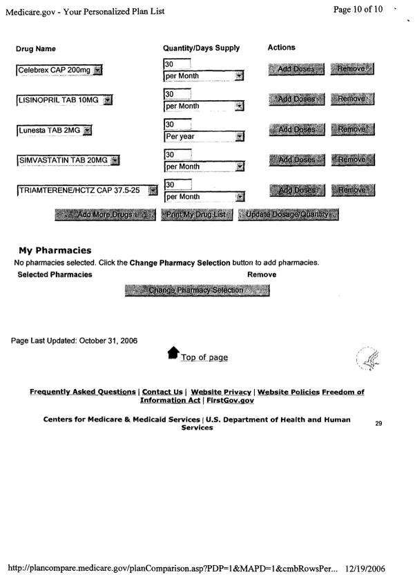
In the baseline survey, the participants answered detailed questions about their prescription drug use and basic questions about personal characteristics. Researchers constructed measures of beneficiary costs in each respondent’s current drug plan and in all available drug plans by entering the respondent’s drug utilization information into the Medicare Plan Finder website. After baseline data were collected, participants were randomly assigned to intervention and comparison groups. Each participant received a personalized mailing. The materials participants received are shown in the Appendix.

The 2007 follow-up inquired about the plan chosen for 2007 and the choice process. 406 people completed the baseline survey, were randomly assigned in the experiment, and completed the 2007 follow-up survey—forming our main analytic sample—and 45 people completed the baseline survey and were assigned to the experiment but could not be reached for follow-up. Thus, although about half of those sent a letter of invitation did not agree to participate (which is relevant for external validity), the study does include 90 percent of people randomly assigned to a group in the experiment (which is particularly relevant for internal validity of the results from the experiment). 92 percent of intervention group and 88 percent of comparison group completed the 2007 follow-up survey.

The 2008 follow-up collected data on drugs used in 2007 and 2008, experiences in the 2007 plan, and the plan chosen for 2008.⁵ 305 of those 406 people completing the 2007 follow-up survey also completed the 2008 follow-up survey.

Data on actual plan enrollment in 2007 (from the 2007 follow-up survey) and 2008 (from the 2008 follow-up survey) was used to determine when individuals had switched plans. To assess the dispersion in costs across plans for the same individuals, we compiled data on the predicted and actual costs of every possible plan. Predicted cost for 2007 is the estimated annual cost measure computed by the Medicare Plan Finder for a given drug plan based on an individual’s prescription drug use as reported at the time of random assignment in fall 2006. The Plan Finder computed the out-of-pocket cost for each plan, assuming that the drugs entered would be taken for the full year of 2007 and that chemically-equivalent generic drugs would be substituted for brand-name drugs. Actual realized cost for 2007 is the estimated annual cost measure computed by the Medicare Plan Finder for a given drug plan based on an individual’s prescription drug use throughout 2007 (with dosages prorated to reflect that cumulative use) as reported at the time of the second follow-up survey in 2008. Predicted cost for 2008 and for 2009 is based on current drug use as reported in the 2008 follow-up survey.

V. Choice Environment

We used our phone survey to assess the context within which seniors made choices about whether or not to change prescription drug plans during open enrollment. A significant majority of respondents knew that different plans were better for different people (82 percent) and that they could only change plans during open enrollment (74 percent). (See Table I.) However, few had learned additional facts about the specific differences among plans. Only 37 percent knew that only some (rather than all) plans have a deductible. Only 55 percent knew that different plans have different co-payments for generic drugs, rather than all plans having the same co-payments.⁶

TABLE I.

Information on Choices from a Nationally Representative Sample, 2007

A. Knowledge of plans
Knew different plans were better for different people	0.82
Knew one could only change plans during open enrollment	0.74
Knew that not all plans have a deductible	0.37
Knew plans have different co-payments for generics	0.55
B. Plan satisfaction and switching
At least somewhat satisfied with 2006 plan	0.85
Switched plans from 2006 to 2007	0.10
C. Information source about plans
Read at least some of Annual Notice of Change	0.57
Ever reviewed mailings for plan choice	0.53
Ever had in-person contact for plan choice	0.14
Ever had phone contact for plan choice	0.07
Ever used internet for plan choice	0.04
Ever reviewed side-by-side comparison for choice	0.34
Ever reviewed personalized information for choice	0.18
Sample size	348

Notes. Data are from a phone survey of Medicare beneficiaries over age 65 who were enrolled in stand-alone Medicare prescription drug plans, as described in section IV. A. The Annual Notice of Change is a mailing from the current plan describing changes in that plan for the coming year.

We found that over 80 percent of respondents were generally satisfied with their 2006 prescription drug plans. The percentage that switched plans between 2006 and 2007 was 10 percent, slightly above the reported national rate of seven percent.⁷ An additional 14 percent considered switching for 2007 but did not switch, which is consistent with the high levels of reported satisfaction.⁸

The leading sources of information that participants used to learn about drug plans were mailings from plans and mailings from Medicare. That material is not personalized and does not convey transparent information about out-of-pocket costs. The more interactive forms of information gathering, such as in-person, phone, or internet, were each used by less than 15 percent of respondents. Eighteen percent reviewed personalized plan comparisons.⁹

To better understand the information available in the existing choice environment and the costs of acquiring it, we audited five potential sources of advice on choosing a drug plan: the Medicare help-line (1–800-Medicare), state health insurance assistance programs (SHIPs), senior centers, other telephone help-lines, and retail pharmacies. In our calls to 1–800-Medicare, customer service representatives consistently entered personalized drug information, identified a low cost plan, and offered to enroll the caller—drawing upon Medicare’s website tool, the Prescription Drug Plan Finder. Our calls to SHIPs generated either referrals to Medicare or offers of similar assistance. Our visits to senior centers sometimes resulted in general discussions about the drug benefit or partial demonstrations of the Medicare website but never in comparative information left in the hands of the auditor. A search for and audit of other sources of telephone advice indicated that few private-sector information sources had emerged.¹⁰ In general, these sources were either not helpful or referred the caller to Medicare or another public-sector information source. In one noteworthy exception (a major pharmacy chain), the help-line offered personalized suggestions, using technology similar to Medicare’s, and mailed a personalized report.¹¹

A small fraction of pharmacies offered personalized in-store assistance with plan choice to auditors who walked in. In four of the 88 pharmacies audited, staff people made personalized plan suggestions based on a Plan Finder. In five pharmacies (all in one chain), a staff person offered personalized plan information about the entire universe of available plans. Sixty-nine of the 88 pharmacies provided print materials. (Separately, tests we gave to recipients of print materials indicated that these materials alone were not sufficient for seniors to understand the cost implications of plan choice even in very simple cases.)

In sum, seniors could acquire personalized assistance from Medicare with minimal effort, but seniors who sought information through other channels were not consistently assisted or even consistently directed to Medicare. Personalized information was readily available but not widely diffused.

VI. Intervention in the Choice Environment

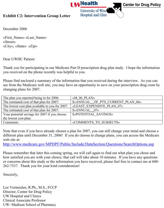
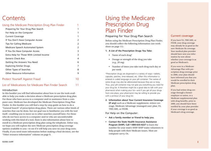
To examine the extent to which a reduction in comparison friction would affect plan choices, we designed a randomized experiment in which the intervention lowered the cost of obtaining and processing the information needed to make comparisons. Members of the intervention group received a one page cover letter showing (1) the individual’s current plan and its predicted annual cost conditional on their personalized drug profile, (2) the lowest-cost plan and its predicted annual cost, (3) the potential savings from switching to the lowest-cost plan, and (4) the date of the end of open enrollment. They also received a printout from the Medicare Plan Finder including costs and other data on all available plans. The comparison group received a general letter referring them to the Medicare website. Both groups received an informational booklet on how to use the site. (For examples of these letters and the booklet, see the Appendix). The intervention included a recommended default option (the lowest-cost plan), a clear statement of that option’s benefits (potential savings), and a deadline. It neither contained difficult to acquire information nor reduced the effort required to change plans.

VI. A. Baseline Characteristics

At the time of the baseline interview, participants reported regularly using an average of five and half medications. The study participants were all from Wisconsin, nearly all white, with an average age of 75. About two-thirds were women, about two-thirds were married, and about half were college graduates (see Table II). Relative to the national population of seniors, study participants were typical in terms of age and gender but were more likely to be married and were substantially better educated.

TABLE II.

Baseline Characteristics for 2007 Wisconsin Follow-up Survey Respondents

	Comparison	Intervention	Difference
	(1)	(2)	(3)
Female	0.63	0.64	0.01 (0.05)
Married	0.67	0.63	−0.04 (0.05)
High school graduate	0.94	0.95	0.01 (0.02)
College graduate	0.47	0.48	0.01 (0.05)
Post-college graduate	0.20	0.16	−0.05 (0.04)
Age 70+	0.78	0.85	0.07 (0.04)
Age 75+	0.45	0.56	0.11* (0.05)
4+ Medications	0.61	0.66	0.04 (0.05)
7+ Medications	0.29	0.33	0.05 (0.05)
2006 plan fair or poor	0.26	0.35	0.09* (0.05)
Predicted consumer cost of baseline plan in 2007	2126	2113	−12 (175)
Cost of lowest-cost plan minus baseline plan in 2007	−520	−533	−13 (62)
Average percentile rank of baseline plan in predicted 2007 consumer cost	37	41	4 (3)

Notes. Data are from a sample of University of Wisconsin Hospital patients, as described in section IV. D. Sample size is 197 in the comparison group and 209 in intervention group. Standard errors are in parentheses.

^*p-value < 0.05

The potential savings from changing plans, as a share of current expenditure, was similar in our intervention sample and in our entirely separate sample of pharmacy claims data—suggesting that the study did not disproportionately attract those who stood to benefit financially from changing plans. Specifically, predicted consumer cost could be reduced an average of 30 percent in our intervention sample by switching to the lowest-cost plan. The corresponding reduction was between 24 and 41 percent in the pharmacy claims sample. (The reason for the range is that among plans offered by a particular plan sponsor, we could not determine the specific plan currently covering an individual in many instances. The smaller potential savings is based on a calculation using the lowest-cost plan among those offered by a sponsor, and the larger potential savings is based on imputation from the sponsor’s highest-cost plan.)

Although the proportional potential savings was similar, the level of expenditure on prescription drugs was substantially higher in our intervention sample than samples more representative of the general population, including our pharmacy claims and national samples. For example, Domino et al. (2008) projected costs under Part D for a nationally representative sample deriving medication usage from the Medicare Expenditure Panel Survey (MEPS). The average 2006 predicted cost in the lowest-cost plan for individuals in the MEPS was $1114, which was 30 percent lower than the corresponding 2007 predicted cost of $1593 for the lowest-cost plans in our intervention sample. That difference is probably due to the intervention sample being drawn from a list of patients with recent clinical visits (and tending to have more health problems and higher levels of prescription drug use), and also to being from a more recent year.

Individual characteristics for the 406 individuals with complete data from both the baseline survey in 2006 and the 2007 follow-up survey were similar for those assigned to the intervention and comparison groups, although the intervention group had a higher fraction age 75 or older and a higher fraction whose satisfaction with their 2006 plan was fair or poor.

VI. B. Percentile Rank in Cost of Chosen Plans

As context for understanding the potential savings from switching plans during open enrollment, we examined the percentile rank in cost of chosen plans in the distribution of available plans, as calculated based on the medication usage reported in our baseline survey. There were 54 Medicare prescription drug plans available to beneficiaries in our Wisconsin sample. The baseline plans initially enrolled in for 2006 by the individuals in our sample were nearer the median-cost plan than the lowest-cost plan among all those offered: the average rank was at the 39^th percentile.

To see how the baseline plans compared to other plans of similar benefit type, we grouped the plans into three different types. “Basic” included: plans with a deductible, 25 percent cost sharing, then a coverage gap, and then catastrophic coverage (known as defined standard plans); actuarially equivalent plans with the same deductible as a defined standard plan but a different cost sharing structure (known as actuarially equivalent standard plans); and actuarially equivalent plans with a reduced or eliminated deductible and a different cost sharing structure (known as basic alternative plans). “Enhanced without gap” included plans with actuarial value exceeding the defined standard plan and no cost sharing in the coverage gap. “Enhanced with gap” included plans with actuarial value exceeding the defined standard plan and with cost sharing in the coverage gap (only for generic drugs, except for one plan).

There is considerable variation in the consumer costs among basic plans, which are identical or actuarially equivalent to the standard plan in terms of insurance value. One plan was the lowest cost of the basic plans for about half the individuals in our sample, but fourteen different plans were the lowest-cost basic plan for others–depending on the drugs they took. On average, the baseline plan was at the 38^th percentile of basic plans (among those who reported enrollment in a basic plan for 2006 in the baseline survey). For individuals with enhanced plans without gap coverage in 2006, the baseline plan was at the 43^rd percentile of predicted consumer costs among plans of that type. For those having enhanced plans with gap coverage in 2006, the baseline plan was at the 50^th percentile of costs among that type of plan. (For analysis of the differences in dollars of cost between baseline plans and the lowest-cost plans by benefit type, see the Appendix.)

In addition to analysis of percentile rank of predicted costs based on drugs taken in 2006, we also examined costs based on the drugs actually taken throughout 2007 as reported in the 2008 follow-up interview. That percentile was similar—37^th for actual costs versus 39^th for predicted costs—when plans of all benefit types were compared. For actual costs among basic plans (among people who had that type plan in 2006), the percentile rank of 35^th was slightly higher than for predicted costs. Among enhanced plans without and with gap coverage (again, among people who had that type of plan in 2006), the percentile ranks were 37^th and 49^th, respectively. Thus, it appears that both ex-ante and ex-post there were numerous options for reducing consumer costs among all plans and among plans of the same benefit type.

VI. C. Intervention Impacts

Switching in 2007

28 percent of those in the group receiving the letter intervention switched plans between 2006 and 2007, compared to 17 percent in the comparison group.¹² The difference of 11.5 percentage points is found in a simple comparison of means (see Table III).

TABLE III.

Regression Coefficients In Models of Plan Switching and Consumer Cost for 2007 Wisconsin Follow-up Survey Respondents

	Switched plan for 2007		Ys − Yb		ln(Ys/Yb)
	(1)	(2)	(3)	(4)	(5)	(6)
Intervention	0.115* (0.041)	0.098* (0.041)	−116* (37)	−103* (37)	−0.065* (0.017)	−0.064* (0.017)
Female		−0.023 (0.045)		−34 (41)		0.008 (0.019)
Married		0.107* (0.045)		−72 (41)		−0.013 (0.019)
High school graduate		−0.044 (0.093)		−45 (84)		−0.005 (0.039)
College graduate		0.048 (0.048)		20 (43)		0.001 (0.020)
Post-college graduate		−0.084 (0.062)		37 (56)		0.029 (0.026)
Age 70+		−0.039 (0.060)		41 (54)		0.054* (0.025)
Age 75+		0.079 (0.048)		−49 (43)		−0.032 (0.020)
4+ Medications		−0.054 (0.050)		−23 (45)		−0.000 (0.021)
7+ Medications		0.116* (0.052)		−112* (47)		−0.008 (0.022)
2006 plan fair or poor		0.097* (0.045)		−55 (41)		−0.010 (0.019)

Notes. Estimates are from linear regression based on equation (4), as described in the text. Y^s is the 2007 predicted consumer cost of the plan selected for 2007. Y^b is that cost for the baseline plan that had been selected in 2006. Sample size is 406. Standard errors are in parentheses.

^*p-value < 0.05

We also estimated the effect of the intervention (Z) on plan switching (D) using linear regression and controlling for covariates (X) known at the time of random assignment—including the age and plan rating variables where there were some differences between the comparison and intervention groups as discussed above—as in equation (4).

$$D_i=Z_i\pi +X_i\beta +{\epsilon }_i$$ (4)

After regression adjustment, the estimated difference is 9.8 percentage points. The probability of such a large difference occurring by chance under the null hypothesis of no effect of the intervention is very small, with p-values less than 0.02 for both specifications. People rating their baseline plan as fair or poor were ten percentage points more likely switch plans, holding other factors constant. The regression-adjusted impact of the intervention on switching is slightly lower than the simple comparison of means primarily because of the interaction between those marginal effects and the higher baseline prevalence of those low satisfaction ratings in the intervention group than in the comparison group.

The average time spent on all aspects of plan consideration and possible switching was 3 hours in the comparison group. Exploring seniors’ choice process and knowledge, we found that several of the differences between the two groups supported the notion that the intervention worked through cognitive channels. These included statistically significantly greater percentages of intervention group members later reporting that they remembered receiving the materials, that they read them, and that they found them helpful.

Predicted 2007 Costs

To estimate effects on costs, we used the same approach as in equation (4) except with change in cost as the dependent variable. Specifically, the change in cost (Y^s − Y^b) is the 2007 predicted consumer cost of the plan selected for 2007 minus that cost for the baseline plan that had been selected in 2006. The average regression-adjusted decrease in predicted cost for the entire intervention group versus the comparison group was $103 (see Table III). Expressed in terms of the change relative to 2006, again estimated using the same approach as in equation (4) but with log of the relative change in cost [ln(Y^s/Y^b)] as the dependent variable, this decrease was an average of 0.064 log points. Again, the probability of such a large difference occurring by chance under the null hypothesis was less than 0.005. (The average cost change for the entire intervention group versus the comparison group averages over people who were not affected by the intervention and those who potentially were affected. Estimates for those affected are discussed in the Appendix.)

Covariates other than the intervention indicator had little power to explain the changes in consumer cost between the baseline 2006 plan and the plan selected in 2007. Holding other factors constant, the indicator for seven or more medications was associated with a reduction in predicted consumer cost of $112, indicating that people with higher levels of medication use chose plans in 2007 resulting in larger reductions in predicted consumer costs than people with less use.

Potential Variability of 2007 Costs

Plans differed in the extent to which costs could be higher or lower if medication use were to change in the future. To create a measure of that potential variability, we used our data on the predicted consumer cost of every plan offered for each of the 406 individuals in our sample. For each plan, we then calculated the difference between the 90^th and 10^th percentiles of the predicted 2007 consumer cost among individuals that reported taking a similar number of medications in the baseline survey. (Specifically, the percentiles were calculated within three subsamples: 0–3 medications, 4–6 medications, and 7 or more medications.) This approach—similar to that used by Abaluck and Gruber (2011)—implicitly assumes that the experiences of other members of our sample with similar medication use represent the range of potential variability for each individual. Because of the small samples sizes used, however, that assumption only holds very roughly, and that measure is also imprecise.

The sample average for that measure of potential variability was about $2900 for the 2006 plans used at the time of the baseline survey. In analysis of the change in that measure between the 2006 plan and the 2007 plan for each individual, using the same approach as in equation (4), potential variability for the intervention group was $10 less than the comparison group (with a standard error of $36). Thus, we did not find evidence that the intervention caused individuals to switch to plans that had greater potential variability according to this measure.¹³

Actual 2007 Costs

In terms of the impacts on consumer cost as measured for the respondents to the 2008 follow-up survey, the predicted 2007 cost was $111 lower for the intervention group and the actual cost was $137 lower—although the standard error was 4 times larger for the impact on actual cost (see Table IV).¹⁴ In addition to allowing more precise estimation, we focused our primary analysis on the predicted 2007 consumer cost of the plan chosen for 2007 rather than the actual 2007 cost because the predicted cost uses the information set available to individuals when they were making their plan choice during open enrollment prior to 2007, which corresponds to the predictable component of costs discussed in section III. Also, the predicted 2007 cost has less attrition, since it is based on our 2007 follow-up survey.

TABLE IV.

Intervention Impacts for 2008 Wisconsin Follow-up Survey Respondents, by Outcome

A. Consumer costs in dollars
Predicted 2007 consumer cost (2007 plan)	−111* (48)
Actual 2007 consumer cost (2007 plan)	−137 (217)
Predicted 2008 consumer cost (2008 plan)	−93 (169)
Predicted 2009 consumer cost (2008 plan)	−159 (170)
B. Quality
Proportion dissatisfied with quality, non-cost features	0.032 (0.033)
Proportion rating overall plan as fair or poor	−0.026 (0.041)

Notes. All estimates are of the coefficient on the intervention indicator from linear regression based on equation (4), as described in the text, using the same vector of covariates as in Table III. Costs are differences from Y^b, the predicted 2007 consumer cost of the 2006 baseline plan. Predicted 2007 costs are based on drugs reported in the baseline 2006 survey. Predicted 2008 and 2009 costs are based on drugs reported in the 2008 follow-up survey. Sample size is 285 in rows 1–3, 241 in row 4, and 302 in rows 5–6. Standard errors are in parentheses.

^*p-value < 0.05

Along with having similar impacts for actual and predicted costs, those two measures were fairly similar at the individual level. The correlation between the actual cost and the predicted cost was 0.68; excluding the three most extreme differences, the correlation between actual and predicted costs was 0.79.¹⁵ Comparing the actual and predicted costs of the 2007 plan selected by the individual, the actual cost was an average of $354 higher than predicted cost among respondents to our 2008 follow-up survey. In the distribution of differences between actual and potential costs, the actual cost was $1872 higher at the 90th percentile, $51 higher at the median, and $663 lower at the 10th percentile.¹⁶

Quality in 2007

Our 2008 follow-up survey also collected self-reported information on experiences in the plan during 2007. There were no statistically significant differences in satisfaction with non-cost features or in overall plan ratings, although the point estimates go in the direction of relatively more dissatisfaction with non-cost features and less dissatisfaction overall for the intervention group (see Table IV). Thus, it is possible that individuals chose lower-cost plans that had lower quality; we do not have sufficient statistical power to reject a hypothesis of small reductions in quality. Analysis of other measures of administrative quality at the plan sponsor level showed essentially no impact.

Switching in 2008

In another assessment of choices from our 2008 follow-up survey, we examined whether individuals were sufficiently satisfied with their choices in 2007 to keep them for 2008 after receiving another opportunity to switch plans. 23 percent of the comparison group switched in 2008, and 20 percent of the intervention group switched—a statistically insignificant difference—implying that the intervention group was at least as satisfied as the comparison group overall in terms of their revealed preferences.

Predicted 2008 and 2009 Costs

The impacts on 2008 and 2009 predicted costs were of roughly the same magnitude as both the predicted and actual costs for 2007 (see Table IV). Like those actual costs, they were imprecisely estimated. We interpret these results as being consistent with continued savings over time due to the intervention, but we also could not reject a null hypothesis of no impact at conventional levels of statistical significance.

VI. D. Role of the Lowest-Cost Plan

We found some evidence that more aspects of the intervention mattered for decision-making than simply the identification of the lowest-cost plan. The intervention letter sent in the fall of 2006 named the plan with the lowest predicted consumer cost in 2007, based on reported prescription drug use, and gave the predicted cost and calculated the difference in cost relative to the 2006 plan. An attachment to the intervention letter also showed the predicted cost of each plan. We found that 9 percent of the intervention group switched specifically to the lowest-cost plans while 20 percent switched to a different plan; in the comparison group these percentages were 2 percent (statistically significantly different from 9 percent) and 15 percent (not statistically significantly different from 20 percent). This result is consistent with the idea that the intervention specifically caused seniors to consider the lowest-cost plan, and also that seniors gave additional consideration to the personalized cost of plans other than the lowest-cost plan.

As a complement to the analysis of the impact of the intervention on switching rates and average predicted costs and to give more structure to the estimated effects, we also examined differences between the intervention and comparison groups in discrete choice models of plan selection. As a point of departure for this analysis, consider selecting a plan at random, which is equivalent to a discrete choice model with coefficients of zero on explanatory variables. The probability of plan selection from among 54 plans would be 1/54 = 0.019. To examine the probability of selecting plans of different prices, we formulated a conditional logit model for individual i and plan j estimated using comparison group data only and controlling for individual fixed effects (α_i), predicted cost (P_ij), and predicted cost squared, based on the indirect utility function in equation (5), with utility ( $u_{ij}^{\ast }$) and an error term (ε_ij).¹⁷

$$u_{ij}^{\ast }=P_{ij}{\beta }_1+P_{ij}^2{\beta }_2+{\alpha }_i+{\epsilon }_{ij}$$ (5)

Results using that model estimate the predicted probability of choosing a plan in 2007 with the same price as that actually selected was 0.025, indicating some sensitivity to price.

We then enriched this basic model, to examine any effect of being the lowest-cost plan (beyond what would be predicted by cost alone) and to analyze differences between the intervention and comparison groups in the sensitivity of plan selection to cost in general and to the lowest-cost plan in particular. The enriched model added an intervention group indicator (Z_i) and interactions of that indicator with predicted cost and predicted cost squared, an indicator for being the lowest-cost plan for that individual (L_ij), and the interaction of lowest-cost plan with the intervention group indicator—as well as 2006 baseline plan choice (B_ij) and plan fixed effects (θ_j), which improve precision of the estimates and also cause plans selected by fewer than 2 individuals in the sample to drop out of this analysis. That model is based on the indirect utility function in equation (6); all explanatory variables in the model were known at the time of random assignment.

$$u_{ij}^{\ast }=P_{ij}{\beta }_1+P_{ij}^2{\beta }_2+L_{ij}{\beta }_3+Z_i{P}_{ij}{\beta }_4+Z_i{P}_{ij}^2{\beta }_5+Z_i{L}_{ij}{\beta }_6+B_{ij}{\beta }_7+{\theta }_j+{\alpha }_i+{\epsilon }_{ij}$$ (6)

We conducted three versions of the analysis based on this equation: plan choices in 2007 for the full sample of 2007 follow-up survey respondents, plan choices in 2007 for the sample of 2008 follow-up survey respondents, and plan choices in 2008 for the full sample of 2008 follow-up survey respondents.

The results for all three versions indicate that the intervention group is significantly more sensitive to cost than the comparison group (see Table V). For the intervention group, the estimates for the first version of the analysis imply that a twenty-five percent decrease in predicted cost (say from $2120 to $1590, or from the 2007 average cost of the plan chosen in 2006 to roughly the average of the lowest-cost plans in 2007—with marginal effects calculated as the sum of 1000 changes of 51.1 cents each) increased the odds of plan selection by 2.7. That is, it increased the probability of selection from 0.025 to 0.070. If that lower cost plan was also the lowest-cost plan, the estimated odds ratio was 8.2, and the probability of selection further rose to 0.27. In the comparison group, a twenty-five percent decrease in predicted cost increased the probability of plan selection only from 0.025 to 0.040. If the lower cost plan was also the lowest-cost plan, the probability of selection further rose only from 0.040 to 0.062 in the comparison group. The test of whether the coefficient on the interaction term of the differential effect of the lowest-cost plan in the intervention group relative to the comparison group was equal to zero generated a p-value of 0.09. A joint test of whether the coefficients on the cost and cost-squared interactions terms were equal to zero also yielded a p-value of 0.09, while the joint test of whether the coefficients on all three cost interactions terms were zero yielded a p-value of less than 0.005. This evidence is consistent with the effect of changes in the choice environment working through both increased sensitivity to the entire vector of costs for all plans and in particular to the lowest-cost plan.

TABLE V.

Conditional Logit Analysis of Plan Selection for Wisconsin Follow-up Survey Respondents

	2007 Plan	2007 Plan	2008 Plan
	(1)	(2)	(3)
β1: 2007 consumer cost/1,000	−1.18 (0.75)	−1.78 (1.05)	−1.63 (0.88)
β2: 2007 (consumer cost/10,000)2	7.69 (6.99)	13.85 (8.90)	14.52 (7.63)
β3: 2007 lowest-cost plan	0.46 (0.60)	0.34 (0.80)	−0.46 (0.73)
β4: 2007 consumer cost/1,000 * intervention	−1.46 (0.94)	−1.10 (1.25)	0.11 (1.11)
β5: 2007 (consumer cost/10,000)2 * intervention	6.92 (8.53)	4.91 (10.68)	−10.33 (10.95)
β6: 2007 lowest-cost plan * intervention	1.16 (0.68)	1.71 (0.89)	3.04* (0.82)
N	12719	7101	7101
Sample limited to 2008 follow-up survey respondents	No	Yes	Yes
p-value on H0: β4 = β5= 0	0.09	0.41	0.15
p-value on H0: β4 = β5 = β6 = 0	0.00	0.02	0.00

Notes. Conditional logit models estimated with individual fixed effects, as in equation (6). Additional coefficients not shown in the table were estimated for the 2006 choice and for each plan; the estimation sample is therefore limited to plans selected by at least 2 individuals in the sample and to individuals choosing a plan selected by at least two individuals. 7 observations with predicted consumer costs > $20k were dropped. Column 1 uses the 2007 follow-up survey respondents, with 401 individuals, 32 plans, and 113 missing cost observations. Columns 2 and 3 use the 2008 follow-up survey respondents, with 265 individuals, 27 plans, and 54 missing cost observations. Standard errors are in parentheses.

^*p-value < 0.05.

The estimates for prediction of 2008 plan selection in the third version of the analysis show that the interactions of cost with the intervention were somewhat smaller and the impact of the lowest-cost plan was somewhat larger than for 2007 plan selection. These results imply that a twenty-five percent decrease in predicted cost in 2007 and being the lowest-cost plan in 2007 increased the estimated odds ratio to 9.9, i.e. the probability of selection in 2008 rose from 0.025 to 0.40. These results are very similar to those from the second version of the analysis, for 2007 plan selection limited to individuals for whom we observe 2008 data, where a twenty-five percent decrease in predicted cost and being the lowest-cost plan increased the probability of selection from 0.025 to 0.38. That is, the 2007 cost information provided in the intervention continued to have an effect of essentially the same magnitude on 2008 plan selection.

VI. E. Impacts on Subgroups

As discussed earlier, our sample was more educated, less satisfied with their baseline plans, and had higher dollar value of potential saving from switching to the lowest-cost plan than a national sample would have had. To examine the sensitivity of our results to these factors, we examined impacts within subgroups by education, plan satisfaction, and potential savings. We also examined the subgroups of people in baseline plans with small and large insurer market shares, and in baseline plans with basic versus enhanced coverage.¹⁸

Education

Our sample is quite highly educated, but estimated impacts for non-college graduates are actually larger than for college graduates, and for both subgroups the null hypothesis of no effect can be rejected at the 5 percent level of significance (see Table VI). These results are consistent with the notion that any limits in comprehending information by less-educated groups are offset by the marginal value of information to these groups.

TABLE VI.

Impacts for 2007 Wisconsin Follow-up Survey Respondents, by Subgroup

	Switching probability		Impact on predicted cost		N
	Comparison	Intervention	Dollars	Log points
	(1)	(2)	(3)	(4)	(5)
A. Education
Not college graduate	0.154	0.284~	−129* (64)	−0.064* (0.025)	213
College graduate	0.183	0.280	−91* (37)	−0.068* (0.024)	193
B. Satisfaction rating of 2006 plan
Fair, poor, or unknown	0.235	0.370	−168 (103)	−0.115* (0.038)	124
Good, very good, or excellent	0.144	0.235~	−73* (32)	−0.046* (0.019)	282
C. Dollar potential savings
≤ $400	0.145	0.217	−32* (16)	−0.052* (0.023)	216
> $400	0.195	0.350~	−176* (77)	−0.075* (0.026)	190
D. Insurer share of sample in 2006
≤ 0.15	0.141	0.333~	−265* (96)	−0.154* (0.031)	142
> 0.15	0.180	0.252	−28 (28)	−0.031 (0.020)	264
E. Benefit type in 2006 baseline
Basic	0.144	0.257~	−85 (44)	−0.061* (0.026)	224
Enhanced (with or without gap coverage)	0.198	0.312	−139* (65)	−0.078* (0.022)	182

Notes. All subgroups are defined on characteristics known prior to random assignment. Dollar potential savings = predicted 2007 consumer cost of 2006 plan - predicted consumer cost of least expensive plan in 2007. ~ = p-value < 0.05 on difference between columns 1 and 2. Columns 3 and 4 are estimated with regression adjustment based on equation (4) using the models in Table III (columns 4 and 6, respectively) estimated separately for each subgroup. Standard errors are in parentheses.

^*p-value < 0.05.

Plan Satisfaction

The proportion of our sample that rated their 2006 baseline plan as fair or poor is much higher than that in national samples (including our telephone survey and data from Medicare) who say they were neither satisfied or dissatisfied, somewhat dissatisfied, or very dissatisfied with their plans. Our sample probably had a high proportion dissatisfied with their plans because they were the people willing to volunteer to participate in our study about drug plan choice. The impacts are larger for the more dissatisfied subgroup (although imprecisely estimated), but quite substantial (and statistically significantly different from zero) even for those who rated their 2006 plan good or better—indicating that the results were not driven primarily by the dissatisfaction of participants with their plans.

Potential Savings

The potential savings from switching to the lowest-cost plan was greater in our sample in dollars and similar in percentage terms to a national sample. The impacts in dollars for those with potential savings less than $400 were much smaller (although statistically significantly different from zero) than for those with greater potential savings. The impacts in relative terms were 0.052 and 0.075 log points for those two groups, respectively. These results suggest that the impact in percentage terms for a sample with nationally representative potential savings would probably have been only slightly smaller than that estimated for the full 2007 Wisconsin follow-up survey sample.

Insurer Market Share

We had initially speculated that individuals with relatively low knowledge of drug plans and drug costs might have placed a high weight on name-recognition and popularity, as potential signals of quality, and had chosen insurers with high enrollment in their plans in 2006. (For example, the plan with the highest national enrollment in 2006 was co-branded by AARP, formerly the American Association of Retired Persons.) We hypothesized that when the intervention made personalized cost information available to individuals in these plans, they would be relatively more likely to switch plans. We found the opposite result. Individuals in plans with insurer market share of less than 15 percent were more likely to respond to the intervention by switching plans and enjoyed greater cost savings. Ex-post, the results are more consistent with the idea that large market share plans attracted members who highly valued a trusted brand or other non-cost attributes and were relatively less sensitive to personalized cost information.

Benefit Type

The impact on switching by benefit type was essentially the same about 11 percentage points. The rate of switching from enhanced plans to enhanced plans was similar in the intervention and comparison groups, but the rate of switching from enhanced to basic plans was much higher in the intervention group. The impact on predicted consumer cost in log points was similar for those with basic and enhanced plans at baseline. The higher level of predicted consumer cost among people with enhanced plans at baseline translated into larger impacts in dollars. In sum, the intervention resulted in lower costs among people with both benefit types at baseline. For those with enhanced plans at baseline, those lower costs appear to have been primarily the result of switching to basic plans.

VI. F. Reduction of Comparison Friction and Stated Preferences

To obtain supplemental evidence about how individuals respond to a reduction in comparison friction, we presented seniors with several sets of plan characteristics including those of the plan they had chosen for themselves and asked them to indicate which they preferred. Following a technique developed by Bernartzi and Thaler (2002), our 2008 follow-up survey asked seniors to evaluate the choice between several pairs of unnamed drug plans based on cost measures, plan size, and Medicare quality ratings. In these questions, the cost information was personalized using the information they had provided about medication use in the 2006 baseline survey and was similar to the information that the intervention group had received via the Medicare printout; the enrollment and quality information were new.

When seniors in the comparison group compared their 2007 plan to their 2006 plan (among those who had changed plans during those years), 61 percent did not select their 2007 plan. When seniors who had not chosen the lowest-cost plan in 2007 were asked to compare their 2007 plan to the lowest-cost plan at that time, 63 percent of the comparison group did not select their 2007 plan. This evidence shows how a reduction in comparison friction (that is, providing personalized information about the unnamed plans) shifted stated preferences away from the actual choices, which is consistent with the substantial impact such a reduction had on actual consumer choices as observed in our field experiment. For the intervention group the analogous results were that 52 percent did not select their 2007 plan over the lowest-cost plan and 16 percent did not select their 2007 plan over their 2006 plan (among those who switched plans), indicating that the shift in stated preferences away from the actual choices was smaller among the intervention group for which comparison friction had been previously reduced during 2006 open enrollment when actual choices were made.

VII. Discussion

We interpret the results of our field experiment to indicate that an intervention which reduced comparison friction had a substantial impact on consumer choices, as it increased the percentage who switched plans from 17 percent to 28 percent and reduced predicted consumer cost by about $100 per person in our Wisconsin sample. Our examination of the choice environment found that information to facilitate comparisons was accessible at quite low cost (say, by calling 1–800-Medicare), but that only 18 percent of individuals nationally had ever used personalized cost information. Why didn’t people seek out and use the available information?

One potential reason people may not have used this information is that the gains are not as large as they appear. Suppose that individuals face high costs from the act of switching plans. The net gains from switching are then smaller than the cost savings alone. This means that the benefits of undertaking comparative research will be lower. Put simply, high switching costs would make it less valuable to investigate options than our cost savings would imply. However, consider the implications if it were the case that essentially all the potential savings from the intervention were offset by switching costs. Say that 17 percent of individuals would have switched if they had been assigned to the comparison group, and therefore would have saved enough to compensate them for switching costs without the intervention; thus, in this case where potential savings are essentially offset by switching costs there would be no effect on potential savings for these individuals because the intervention did not cause them to switch or increase switching costs. Then the intervention caused only 10 percent of individuals to switch plans. In this case then the overall effect of $103 per person in potential savings from receiving a letter would have been a combination of no effect on 90 percent of individuals and $1030 per person caused to switch. Since the act of switching itself could be accomplished in a phone call, this case seems implausible and we conclude such switching costs were very unlikely to have fully offset the potential savings from the intervention. Switching costs less than $100 per person caused to switch seem more plausible.

Individuals may have expected the costs of understanding the forms and adjusting to the procedures of a new plan to be higher than the costs directly related to the act of switching. That uncertainty is a form of comparison friction that our intervention—which focused on premiums plus out-of-pocket expenditures—did not reduce. If individuals had greater knowledge of these factors for their current plan and did not have an effective way to learn about them for other plans, then again the net benefits of alternative choice would have been lower and comparative research would have been less likely to be worthwhile. These factors probably contributed to the low use of personalized cost information.

In our view, a key reason people did not seek personalized comparative information was that they had biased expectations about how much they could save from switching plans. We asked participants in the comparison group during our 2007 follow-up interview how much they thought they could save if they had chosen the least expensive plan. Of those who could give an estimate, more than 70 percent gave an underestimate, and the average underestimate was more than $400. Because they thought the value of comparative research was going to be low, they did not undertake it.

Biased expectations about costs may have combined with confirmation and status-quo biases (the tendency to stick with one’s existing opinions and choices), procrastination, limited attention, and small transaction costs to generate high rates of reported satisfaction and low rates of change. Our intervention, while modest, challenged these tendencies by altering price and market perceptions, countering confirmation bias (by showing the savings available), and providing an alternative default (the lowest-cost plan). Our results suggest that the mechanisms underlying the intervention impact increased sensitivity to plan cost in general, and to the lowest-cost plan highlighted in the letter in particular.

VIII. Directions For Further Research

This study highlights four areas for further research. One is very concrete work on the design of clear, actionable information about Medicare drug plans or other health insurance coverage choices. Our work shows the potential for information to have an effect, although the study intervention incorporated multiple features including partnership with a trusted hospital, the priming effect of an in-person interview, a behaviorally sensitive letter, the full Medicare printout, and a mailing that both communicated personalized information about potential savings and raised general awareness about the potential for savings and the nature of the variation among plans. Additional work could unbundle these effects, with potential implications for the design of larger scale programs, and could explore the effects of quality as well as cost information. Tools for creating more sophisticated price information could also be developed that would incorporate, for example, forecasts of changes in drug use, rather than simply assume that next year’s use will be the same as the previous year’s use.

Another area for further research is the role of product and information markets in reducing comparison friction. It is striking that, despite the apparent value of personalized comparative information, few third parties emerged to provide it, or even to highlight its potential value and steer seniors towards Medicare and its local partners. The actual provision of information may have been impeded by CMS regulations that constrained the role of third parties and by the effort involved in working with seniors one-on-one, although third parties with access to drug histories can provide personalized information relatively efficiently. Among the challenges in facilitating an expanded role for third parties would be the need to minimize the potential for plans to capture the market for advice, to respect individual privacy, to provide information that balanced cost and other considerations, and to hold beneficiaries’ well-being as the greatest value. Possibilities to explore could be one-on-one counseling and the ability for beneficiaries and their advisors to manually update an automatically generated drug list.

A third area involves the potential response of insurance firms to broader provision of personalized price information. For example, if the information provided assumed last year’s drug use is the same as next year’s drug use, then firms would have strong incentives to cut prices on drugs used for short periods and increase prices on drugs used for long periods to encourage individuals to perceive their costs to be lower than they would actually be. In contexts of increased price salience, there would also be greater incentives for firms to cut costs which could lead to lower overall quality of service.

A fourth area for more conceptual research is the interaction between comparison friction and various forms of market failure at both the theoretical and the more practical level. In the case of Medicare drug plans, the private and public optima may differ, and comparison friction may actually counteract market failure by reducing the extent of adverse selection and contributing to the success of the voluntary insurance market. Market functioning could be harmed if all plans with more than basic coverage attract only those for whom those plans are least costly (with these plans then becoming too expensive and being dropped), or if all individuals chose one low-cost provider who then obtained enough market power to keep out new entrants and also set monopolistic prices in future periods.

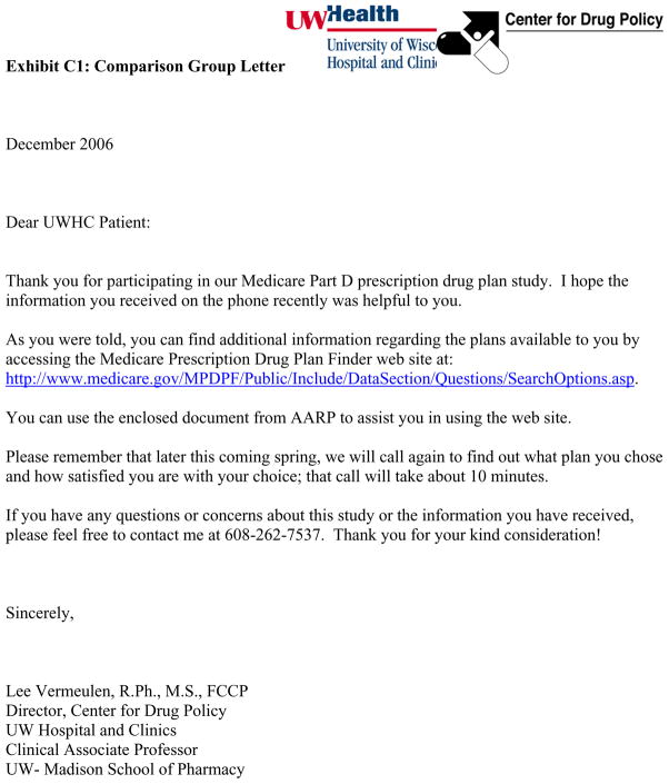
Exhibit C1.

Comparison Group Letter

Exhibit C2.

Intervention Group Letter

Exhibit C3.

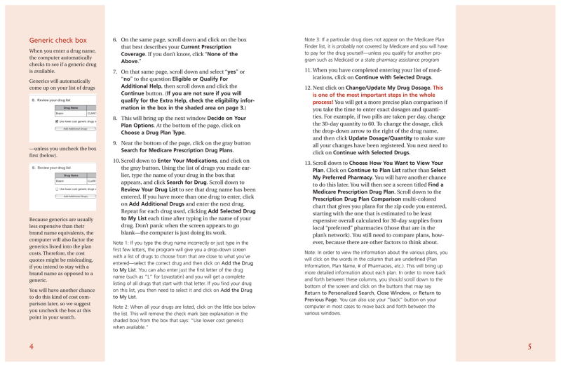
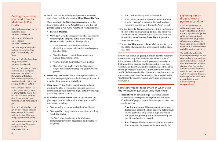
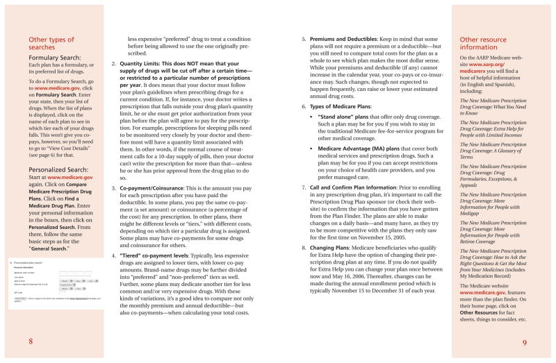
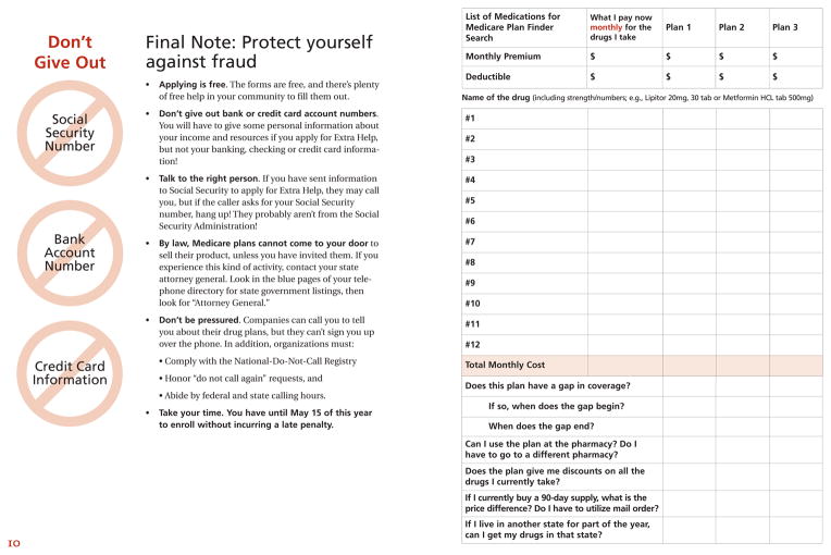
Booklet provided The New Medicare Prescription Drug Coverage: Using the Medicare Prescription Drug Plan Finder

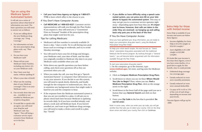
Exhibit C4.

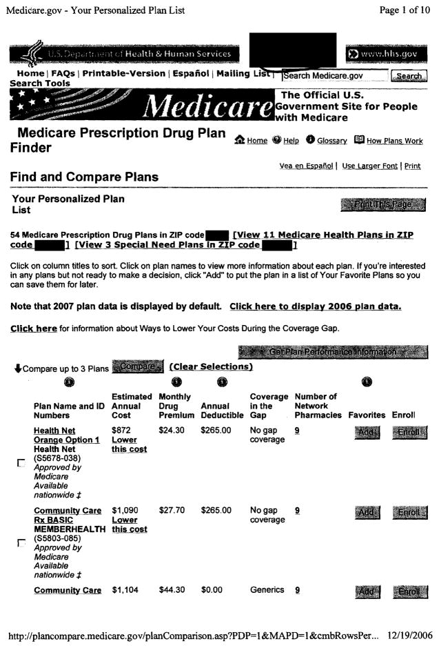
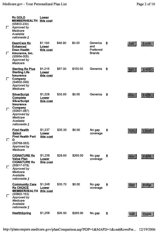
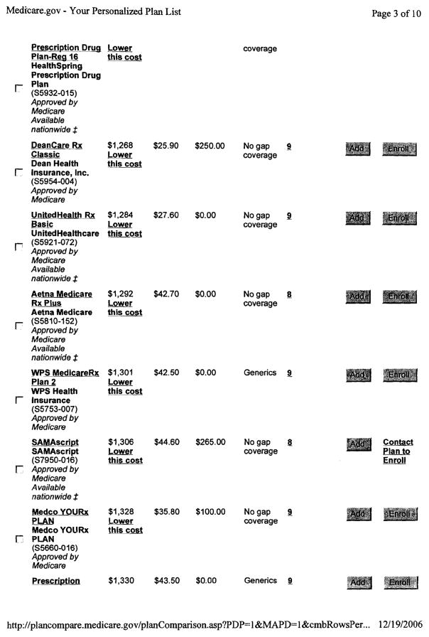
Medicare Prescription Drug Plan Finder Printout

Appendix

A. Potential cost savings from plan switching by benefit type

Using data from the baseline survey on drugs taken in 2006, the average predicted consumer savings from switching to the lowest-cost plan in 2007 of any benefit type was $527. Those savings from switching to the lowest-cost plan of the same benefit type as the individual had in 2006 ranged from $386 to $464 (see Table A-1).

TABLE A-1.

Average Difference in Cost between Baseline Plan and Lowest-Cost 2007 Plan

	Dollars		Percentile Rank
	Potential	Actual	Potential	Actual
	(1)	(2)	(3)	(4)
Among Basic Plans	−386	−337	38	35
Among Enhanced Plans Without Gap Coverage	−429	−391	43	37
Among Enhanced Plans With Gap Coverage	−464	−392	50	49
Among All Plans	−527	−487	39	37

Notes. The baseline plan is the plan in which the individual was enrolled in 2006. The dollar difference is the cost in 2007 of lowest-cost plan minus that of the baseline plan. The percentile rank the rank of the cost of the lowest-cost plan minus the baseline plan (where zero provided the most savings and 100 provided the least savings). The sample for rows 1–3 is limited to plans of the same type as the baseline plan. The sample size for potential costs was 224, 73, 109, and 406 for rows 1–4 respectively in columns 1 and 3; for actual costs it was 155, 58, 85 and 298 for those rows in columns 2 and 4.

We also examined information on drugs actually taken in 2007 from our 2008 follow-up survey. The average actual savings from switching to the lowest-cost plan in 2007 of any benefit type was $487. Those savings from switching to the lowest-cost plan of the same benefit type as the individual had in 2006 ranged from $337 to $392.

The average consumer cost among all 2007 basic plans was $2334. In comparison to the lowest-cost basic plan for each individual, the 27 other basic plans had predicted consumer costs $705 greater on average.

B. Intervention impacts assuming some participants were not affected

The intervention impacts on predicted consumer cost discussed in the main text are intent-to-treat estimates which compare the outcomes for all members of the intervention group to those of the comparison group. However, the change in predicted consumer cost is zero by definition for individuals who did not switch plans. Thus, the intent-to-treat estimates average together impacts on those potentially affected by the intervention with a large proportion of zeros for those not affected. This section explores how different assumptions about the proportion of the sample not affected scales up the point estimates and standard errors of those who were potentially affected.

Define A as an indicator of being potentially affected by the intervention, where A involves the counterfactual and cannot be directly observed. Define D as an observed indicator for switching plans, and Z as an indicator for assignment to the intervention group. Define Y as the difference in predicted consumer cost of the plan selected for 2007 and the baseline plan in 2006, Y₁ as the potential outcome if an individual were assigned to the intervention group, Y₀ as the potential outcome if an individual were assigned to the comparison group. The causal effect of the intervention is then Y₁−Y₀.

There was a causal effect for any individual who would have chosen a plan with a different predicted consumer cost in the intervention group than in the comparison group. These situations included having the intervention cause someone to switch to a lower cost plan (Y₁<0; Y₀=0), having the intervention cause someone who was going to choose a more expensive plan to not switch (Y₁=0; Y₀>0), and other cases (anytime Y₁ ≠ Y₀). A special case was when someone would not switch plans regardless of the intervention, so there was no effect on cost. The upper bound on the probability of this special case occurred when everyone who switched plans in one group would have switched if assigned to the other group (1 − max{E[D | Z=1], E[D | Z=0]}). The lower bound on the probability of this special case occurred when no one who switched plans in one group would have switched if assigned to the other group (1 − {E[D | Z=1] + E[D | Z=0]}). Intuitively, we can use the lower bound on the fraction of zeros included in the estimate of the average cost change for the entire intervention group versus the comparison group to calculate a lower bound on the average cost change for those who potentially were affected by the intervention. This bound is based on the derivation in equation (B1).¹⁹

$$\begin{array}{l}\text{E}[{\text{Y}}_1\mid \text{Z}=1]-\text{E}[{\text{Y}}_0\mid \text{Z}=0]\\ =\text{E}[{\text{Y}}_1-{\text{Y}}_0]\\ =\text{E}[{\text{Y}}_1-{\text{Y}}_0\mid \text{A}=1]Pr(\text{A}=1)+\text{E}[{\text{Y}}_1-{\text{Y}}_0\mid \text{A}=0]Pr(\text{A}=0)\\ =\text{E}[{\text{Y}}_1-{\text{Y}}_0\mid \text{A}=1]Pr(\text{A}=1)+0\\ \le \text{E}[{\text{Y}}_1-{\text{Y}}_0\mid \text{A}=1]\{\text{E}[\text{D}\mid \text{Z}=1]+\text{E}[\text{D}\mid \text{Z}=0]\}\end{array}$$ (B1)

This approach is similar to that used by Imbens and Angrist (1994) to estimate a local average treatment effect (LATE), where those who did not comply and take up the treatment offer are assumed to have been unaffected. However, the approach used here is less restrictive. The exclusion restriction required for LATE, but not needed for (B1), is that people who would have switched plans even without the intervention would not be affected; relaxing this assumption is sometimes described as allowing effects on “always-takers.” LATE also involves an assumption of monotonicity, not needed for (B1), where the intervention only encourages switching; relaxation of this assumption is sometimes referred to as allowing “defiers.” We can now calculate an expression based for a lower bound on the average cost change for those who were potentially affected by the intervention, shown in equation (B2).

$$\text{E}[{\text{Y}}_1-{\text{Y}}_0\mid \text{A}=1]\ge \{\text{E}[\text{Y}\mid \text{Z}=1]-\text{E}[\text{Y}\mid \text{Z}=0]\}/\{\text{E}[\text{D}\mid \text{Z}=1]+\text{E}[\text{D}\mid \text{Z}=0]\}$$ (B2)

In this paper’s application, the lower bound point estimates and standard errors simply rescale the intent-to-treat estimates by 1/{E[D | Z=1] + E[D | Z=0]}, or 2.2 (see Table B-1). There is a small amount of negative covariance between the estimation of average cost differences and switching rates, and accounting for this slightly reduces the standard errors; for simplicity, this adjustment is not included in the results.

TABLE B-1.

Intervention Impacts in the Wisconsin 2007 Follow-up Survey Assuming Some Participants Were Not Affected, by Subgroups

	Lower bound impact on predicted cost		Treatment-On-Treated impact on predicted cost		N
	Dollars	Log points	Dollars	Log points
	(1)	(2)	(3)	(4)	(5)
A. Education
Not college graduate	−295* (147)	−0.146* (0.057)	−454* (226)	−0.224* (0.088)	213
College graduate	−196* (80)	−0.146* (0.053)	−325* (132)	−0.242* (0.087)	193
B. Satisfaction rating of 2006 plan
Fair, poor, or unknown	−278 (171)	−0.189* (0.062)	−455 (279)	−0.310* (0.102)	124
Good, very good, or excellent	−192* (85)	−0.122* (0.050)	−310* (137)	−0.196* (0.081)	282
C. Dollar potential savings
≤ $400	−88* (45)	−0.143* (0.064)	−148* (75)	−0.238* (0.106)	216
> $400	−323* (141)	−0.137* (0.048)	−503* (220)	−0.214* (0.075)	190
D. Insurer share of sample in 2006
≤ 0.15	−559* (203)	−0.324* (0.065)	−795* (289)	−0.461* (0.093)	142
> 0.15	−65 (64)	−0.073 (0.047)	−112 (110)	−0.125 (0.081)	264
E. Benefit type in 2006 baseline
Basic	−211 (111)	−0.152* (0.065)	−330 (173)	−0.237* (0.101)	224
Enhanced (with or without Gap Coverage)	−272* (127)	−0.153* (0.044)	−445* (208)	−0.249* (0.072)	182
F. All
Full sample	−229* (83)	−0.143* (0.038)	−365* (132)	−0.228* (0.061)	406

Notes. Estimates are with regression adjustment using the models in Table III, columns 4 and 6, estimated separately for each subgroup, and modified as follows: columns (1) and (2) are based on equation (B2), and multiply the estimates by 1/(0.282+0.168); columns (3) and (4) are based on equation (B3), and multiply the estimates by 1/0.282. All subgroups are defined on characteristics known prior to random assignment. Dollar potential savings = predicted 2007 consumer cost of 2006 plan - predicted consumer cost of least expensive plan in 2007. Standard errors are in parentheses.

^*p-value < 0.05.

Our intuition is that the exclusion restriction does not hold in this application but monotonicity probably does. The exclusion restriction would be violated if those in the comparison group who would have switched without the intervention nevertheless had their predicted consumer cost affected by the intervention. Monotonicity would be violated if the intervention caused some people to not switch who would have otherwise switched. If we did not impose the exclusion restriction but assume monotonicity holds—that is, allow effects on “always-takers” but assume no “defiers”—then then we would obtain treatment-on-treated results from rescaling by 1/E[D | Z=1] instead of 1/{E[D | Z=1] + E[D | Z=0]}, as in equation (B3).

$$\text{E}[{\text{Y}}_1-{\text{Y}}_0\mid \text{A}=1]=\{\text{E}[\text{Y}\mid \text{Z}=1]-\text{E}[\text{Y}\mid \text{Z}=0]\}/\{\text{E}[\text{D}\mid \text{Z}=1]\}$$ (B3)

Estimates of treatment-on-treated effects based on (B3) generate point estimates about 3.6 times larger than the lower bound on the potentially affected group based on (B2).

The regression-adjusted estimate of the treatment-on-treated effect for the full sample is $369 (see Table B-1). That turns out to be very similar to the non-experimental estimate that compares the savings of those who switched plans in the intervention group (who had potential savings that averaged $469) to those who switched plans in the comparison group (who had potential savings that averaged $97), where the difference is $372. Because the potential savings for non-switchers is zero by construction, if there were no regression adjustment and the switching rates in the two groups were the same then treatment-on-treated estimate would exactly equal the difference between switchers in potential savings; in this application, the regression adjustment and lower switching rate in the comparison group roughly offset each other.

References

- Abaluck Jason, Gruber Jonathan. Choice Inconsistencies Among the Elderly: Evidence from Plan Choice in the Medicare Part D Program. American Economic Review. 2011 June;101(4):1180–1210. doi: 10.1257/aer.101.4.1180. [DOI] [PMC free article] [PubMed] [Google Scholar]
- Bernartzi Shlomo, Thaler Richard H. How Much is Investor Autonomy Worth? Journal of Finance. 2002;57(4):1593–1616. [Google Scholar]
- Brown Jeffrey R, Goolsbee Austan. Does The Internet Make Markets More Competitive? Evidence From The Life Insurance Industry. Journal of Political Economy. 2002 June;110(3):481–507. [Google Scholar]
- Brynjolfsson Erik, Smith Michael D. Frictionless Commerce? A Comparison of Internet and Conventional Retailers. Management Science. 2000 April;46(4):563–585. [Google Scholar]
- Bundorf M Kate, Szrek Helena. Choice Set Size and Decision Making: The Case of Medicare Part D Prescription Drug Plans. Medical Decision Making. 2010 September/October;30:582–593. doi: 10.1177/0272989X09357793. [DOI] [PMC free article] [PubMed] [Google Scholar]
- Domino Marisa Elena, Stearns Sally C, Norton Edward C, Yeh Wei-Shi. Why Using Current Medications to Select a Medicare Part D Plan May Lead to Higher Out-of-Pocket Payments. Medical Care Research and Review. 2008 February;65(1):114–126. doi: 10.1177/1077558707307577. [DOI] [PubMed] [Google Scholar]
- Duggan Mark G, Morton Fiona Scott. The Medium Term Impacts of Medicare Part D on Pharmaceutical Prices. American Economic Review: Papers and Proceedings. 2011 May;101(3):387–392. doi: 10.1257/aer.100.1.590. [DOI] [PubMed] [Google Scholar]
- Ellison Glenn, Ellison Sara Fisher. Search, Obfuscation, and Price Elasticities on the Internet. Econometrica. 2009 March;77(2):427–452. [Google Scholar]
- Engelhardt Gary V, Gruber Jonathan. Medicare Part D and the Financial Protection of the Elderly. American Economic Journal: Economic Policy. forthcoming. [Google Scholar]
- Fung Archon, Graham Mary, Weil David. Full Disclosure: The Perils of and Promise of Transparency. Cambridge, England: Cambridge University Press; 2007. [Google Scholar]
- Gold Marsha, Achman Lori, Brown Randall S. The Salience of Choice for Medicare Beneficiaries. Managed Care Quarterly. 2003 Winter;11(1):24–33. [PubMed] [Google Scholar]
- Goldman Dana P, Joyce Geoffrey F, Vogt William B. Part D Formulary and Benefit Design as a Risk Steering Mechanism. American Economic Review: Papers and Proceedings. 2011 May;101(3):382–386. doi: 10.1257/aer.101.3.382. [DOI] [PMC free article] [PubMed] [Google Scholar]
- Hanoch Yaniv, Rice Thomas, Cummings Janet, Wood Stacey. How Much Choice Is Too Much? The Case of the Medicare Prescription Drug Benefit. Health Services Research. 2009 August;44(4):1157–1168. doi: 10.1111/j.1475-6773.2009.00981.x. [DOI] [PMC free article] [PubMed] [Google Scholar]
- Hastings Justine S, Weinstein Jeffrey M. Information, School Choice, and Academic Achievement: Evidence from Two Experiments. Quarterly Journal of Economics. 2008 November;123(4):1373–1414. [Google Scholar]
- Heiss Florian, McFadden Daniel, Winter Joachim. Who Failed to Enroll in Medicare Part D, and Why? Health Affairs. 2006 August;25(5):w344–w354. doi: 10.1377/hlthaff.25.w344. [DOI] [PubMed] [Google Scholar]
- Heiss Florian, McFadden Daniel, Winter Joachim. Mind the Gap! Consumer Perceptions and Choices of Medicare Part D Prescription Drug Plans. In: Wise David A., editor. Research Findings in the Economics of Aging. Chicago, IL: University of Chicago Press; 2010. pp. 413–481. [Google Scholar]
- Hibbard Judith H, Slovic Paul, Peters Ellen, Finucane Melissa L, Tusler Martin. Is The Informed-Choice Policy Approach Appropriate For Medicare Beneficiaries? Health Affairs. 2001 May/June;20(3):199–203. doi: 10.1377/hlthaff.20.3.199. [DOI] [PubMed] [Google Scholar]
- Ketcham Jonathan D, Lucarelli Claudio, Miravete Eugenio J, Christopher Roebuck M. unpublished manuscript. University of Texas; Austin: Dec, 2010. Sinking, Swimming, or Learning to Swim in Medicare Part D. [Google Scholar]
- Lucarelli Claudio, Prince Jeffrey, Simon Kosali. Measuring Welfare and the Effects of Regulation in a Government-Created Market: The Case of Medicare Part D Plans. NBER Working Paper No. w14296. 2008 September; [Google Scholar]
- McCormack Lauren A, Garfinkel Steven A, Hibbard Judith H, Kilpatrick Kerry E, Kalsbeek William D. Beneficiary Survey-Based Feedback on New Medicare Information Materials. Health Care Financing Review. 2001 Fall;23(1):37–46. [PMC free article] [PubMed] [Google Scholar]
- MedPAC. Report to the Congress: Medicare Payment Policy. Washington, DC: Medicare Payment Advisory Commission; 2007. [Google Scholar]
- Neuman Patricia, Strollo Michelle Kitchman, Guterman Stuart, Rogers William H, Li Angela, Rodday Angie Mae C, Safran Dana Gelb. Medicare Prescription Drug Benefit Progress Report: Findings From a 2006 National Survey of Seniors. Health Affairs. 2007;26(5):w630–w643. doi: 10.1377/hlthaff.26.5.w630. [DOI] [PubMed] [Google Scholar]
- Morton Scott, Fiona Florian Zettelmeyer, Silva-Risso Jorge. Internet Car Retailing. The Journal of Industrial Economics. 2001 December;49(4):501–519. [Google Scholar]
- U.S. Department of Health and Human Services. [accessed July 22, 2011];Medicare Drug Plans Strong and Growing. 2007 January 30; press release, http://www.cms.hhs.gov/apps/media/press/release.asp?Counter=2079.
- Weil David, Fung Archon, Graham Mary, Fagotto Elena. The Effectiveness of Regulatory Disclosure Policies. Journal of Policy Analysis and Management. 2006;25(1):155–181. [Google Scholar]
- Winter Joachim, Balza Rowilma, Caro Frank, Heiss Florian, Jun Byung-hill, Matzkin Rosa, McFadden Daniel. Medicare Prescription Drug Coverage: Consumer Information and Preferences. Proceedings of the National Academy of Sciences. 2006 May 16;103(20):7929–7934. doi: 10.1073/pnas.0601837103. [DOI] [PMC free article] [PubMed] [Google Scholar]
- Yin Wesley, Basu Anirban, Zhang James X, Rabbani Atonu, Meltzer David O, Alexander G Caleb. The Effect of the Medicare Part D Prescription Benefit on Drug Utilization and Expenditures. Annals of Internal Medicine. 2008 February 5;148(3):169–177. doi: 10.7326/0003-4819-148-3-200802050-00200. [DOI] [PubMed] [Google Scholar]
- Imbens Guido W, Angrist Joshua D. Identification and Estimation of Local Average Treatment Effects. Econometrica. 1994 March;62(2):467–476. [Google Scholar]