Measuring Membrane Protein Dynamics in Neurons Using Fluorescence Recovery after Photobleach

Abstract

The use of genetically encoded fluorescent tags such as green fluorescent protein (GFP) as reporters to monitor processes in living cells has transformed cell biology. One major application for these tools has been to analyze protein dynamics in neurons. In particular, fluorescence recovery after photobleach (FRAP) of surface expressed fluorophore-tagged proteins has been instrumental to addressing outstanding questions about how neurons orchestrate the synaptic delivery of proteins. Here, we provide an overview of the methodology, equipment, and analysis required to perform, analyze, and interpret these experiments.

1. Introduction

Cells are highly dynamic structures and their constituent protein components are in constant motion within and between cellular compartments, domains, and microdomains. Membrane spanning proteins such as receptors and ion channels oscillate between confined and free Brownian motion (Meier et al., 2001; Serge et al., 2002). These processes are important because they participate in the localization of proteins to the appropriate regions of the cell surface. This is especially critical in neurons, which are highly polarized and morphologically complex cells that transmit and process information via synaptic transmission. Each neuron can receive information via thousands of synapses and each Individual synapse requires the precise, activity-dependent, and coordinated delivery, retention, and removal of specialized sets of proteins.

1.1. Fluorescent probes

Green fluorescent protein (GFP) and subsequent derivatives and alternatives (Pakhomov and Martynov, 2008; Tsien, 1998) are bright, stable, nontoxic fluorophores that allow prolonged imaging of protein trafficking in live cells. Crucially, virtually any protein can be tagged with GFP resulting in a fusion that usually retains the same targeting and functional properties as the parent protein when expressed in cells. A potential limitation of most GFP-derived or -related fluorophores, however, is that they are fluorescent as soon as the protein is folded and remain fluorescent until degraded. Thus, fluorescent molecules can be found at all stages of the protein production pathway from early after synthesis until degradation. Therefore, an important experimental consideration is that the compartmental localization of the fluorescent signal corresponds to the main site of residence of the mature protein. To circumvent these complications, GFP family proteins have been engineered to generate a range of mutants with specifically altered properties such as shifts in emission wavelength or pH sensitivity (Table 6.1).

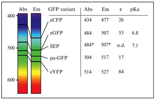
Table 6.1.

Properties of GFP derivatives

Compiled maximum absorbance and emission wavelength for eCFP (enhanced cyan fluorescent protein), eGFP (enhanced green fluorescent protein), SEP (superecliptic pHluorin), pa-GFP (photoactivable GFP), and eYFP (enhanced yellow fluorescent protein). On the left, values are pointed on spectral bands. Also given are the molar extinction coefficient and pKa.

Abs, maximum absorbance in nm; Em, maximum emission in nm; ε, molar extinction coefficient in 10³ M⁻¹ cm⁻¹.

^*denotes when fluorescence not eclipsed by acidic pH.

Data taken from Ashby et al. (2004a); Miesenbock et al. (1998); Pakhomov and Martynov (2008); Sankaranarayanan et al. (2000).

Among these, superecliptic pHluorin (SEP), a pH-sensitive derivative of eGFP, has been extensively used for live cell imaging of plasma membrane proteins (Ashby et al., 2004b; Sankaranarayanan et al., 2000). Protonation of SEP decreases photon absorption and therefore eliminates fluorescence emission at low pH. This allows the selective imaging of tagged proteins exposed to neutral pH environment. This is useful because most stages of the secretory pathway in neurons and other cells occur in acidic compartments, so a SEP-tagged membrane protein absorbs and emits fluorescence only when inserted in the plasma membrane (Ashby et al., 2004b).

Quantification of the pH-dependence of SEP fluorescence suggests that it is 21× brighter at pH 7.4 than at 5.5 (Sankaranarayanan et al., 2000). Thus, if only ~5% of the SEP is surface expressed and exposed to pH 7.4 and 95% is intracellular and exposed to pH 5.5, there will be the same levels of fluorescence signal from the cell surface and inside the cell. This is an important issue to be aware of and control for with acid and ammonium chloride wash protocols (see Section 5) that specifically identify the contributions of surface expressed and intracellular proteins. Fortunately, our experience in neurons is that recombinantly expressed SEP-tagged surface membrane proteins produce bright signals with a very good signal to noise ratio, meaning that surface expressed fluorophore can be readily distinguished (Ashby et al., 2004a, 2006;Bouschet et al., 2005; Jaskolski et al., 2009; Martin et al., 2008).

1.2. Photobleaching and recovery

Like other fluorescent dyes, when illuminated at high intensity, GFP derivatives can be irreversibly bleached without detectably damaging intracellular structures (Patterson et al., 1997; Swaminathan et al., 1997; Wiedenmann et al., 2009). As SEP only absorbs photons when exposed to neutral pH, it allows the selective bleaching of only SEP-tagged plasma membrane proteins (Ashby et al., 2004a, 2006; Bouschet et al., 2005; Jaskolski et al., 2009; Martin et al., 2008). Fluorescence recovery after photobleach (FRAP) relies on the high mobility of cellular proteins under physiological conditions within the plasma membrane; proteins undergo various types of motion from free diffusion to flow motion and/or anchoring (see Jaskolski and Henley, 2009). When fluorescently tagged proteins are bleached in a region of interest (ROI), the recovery in fluorescence occurs due to the movement of unbleached SEP-tagged protein from areas outside the ROI into the bleached region. At the same time, bleached SEP-tagged protein within the ROI moves out of the ROI (Fig. 6.1A). Thus, FRAP is a convenient and powerful technique to assess protein movement, and the fact that SEP is fluorescent predominantly when located only at the plasma membrane allows experiments to focus on the properties of surface expressed proteins.

Figure 6.1.

Fluorescence recovery after photobleaching, theory, and analysis. (A) Schematic representing successive steps of a FRAP experiments using SEP-tagged proteins. A fraction of tagged proteins undergoes motion in the plasma membrane, while another fraction is clustered and thus immobilized (red dot). Left column, simulated FRAP images, t–1 is the prebleach step, t0 is the bleach step (see black bleached proteins), t1 is the initial recovery due to lateral diffusion (black double arrow), t2 corresponds to the steady state late recovery where only immobile proteins (red dot) remains within the bleached area. The right-hand panels show corresponding stages of FRAP in dendritic spines. In the top panel, the white arrows indicate the bleached spines and the red arrow a control spine. The scale bar is 1 μm. (B) A typical FRAP recording and formulas for curve fitting (according to Feder et al. 1996) and diffusion coefficient calculus (see analysis section). (C) Complex membrane area approximation using calibration curves. Dendrites with spines of membrane-anchored eGFP-expressing neuron. A nonspiny region of the shaft is cropped and aligned, and fluorescence is measured for various lengths (L). Using the width (w) of the shaft, the area of a corresponding cylinder is computed. Left, fluorescence is plotted versus calculated area to produce a calibration curve. Membrane area of labeled spines (1–4) can be read on the curve.

2. Experimental Parameters and Preparation

2.1. Buffer composition

Bicarbonate-based solutions that are typically used for culturing cells are not usually used for short-term imaging experiments because of the practical difficulty of maintaining CO₂/O₂ balance. Further, it is also advisable to avoid the use of phenol red and serum since both are sources of fluorescence.

The buffer we use for cell culture is GIBCO™ Neurobasal™ Medium (1×) supplemented with 2% of B-27 and 0.5 mM glutamine or Glutamax. The composition of imaging buffer is NaCl 119 mM; Hepes 25 mM; Glucose 10 mM; NaHCO3 1–2 mM; KCl 2.5 mM; NaH2PO4 1mM; CaCl2 1.8–2.5 mM; MgSO4 0.8–1.3 mM; adjust the pH to 7.4. For low pH solution, HEPES was replaced with equimolar MES and pH was adjusted to 6.0.

2.2. Temperature

Temperature affects the mobility of both soluble and membrane-associated molecules. Because viscosity is highly dependent on temperature, the effects on diffusion can be striking (Reits and Neefjes, 2001). Thus the temperature of the cells being imaged needs to be constant, for example, on a controlled temperature stage, ideally at a physiological temperature. It should also be noted that temperature fluctuations of the stage and objective can cause focus drift. To limit the impact of this variable, the imaging set up should be switched on and warmed up for 30 min prior to the experiment.

2.3. Osmolarity

Alterations in cell volume caused by hypo/hyperosmolarity can profoundly alter cell function (Sabirov and Okada, 2009). Changes in the osmolarity can occur during the experiment due to evaporation of the medium and/or differences in the composition of the culture media and the recording media. It is therefore necessary to determine the osmolarity of the culture media and adjust the osmolarity of the recording media accordingly and evaporation should be minimized by using a humidified environment.

2.4. Health and viability of cells

Our FRAP experiments are performed using dispersed cultures of hippocampal neurons (Ashby et al., 2004a, 2006; Jaskolski et al., 2009; Martin et al., 2008). Cell morphology can be assessed using transmitted-light microscopy techniques to identify cells that are stressed, dying, or dead before starting the experiment. The formation of irregular plasma membrane bulges, large vacuoles, and detachment from the tissue-culture plate are all indicators of cell stress. In addition, clustering of the fluorescent signal is a strong indication that cells are under stress (Samhan-Arias et al., 2009) (Fig. 6.2). Another key indicator of stressed neurons is compromised membrane integrity, which is routinely assessed in the FRAP experiment using SEP by brief acid and ammonium chloride washes (see Section 5).

Figure 6.2.

Examples of damaged neurons. These are 21 DIV hippocampal neurons expressing a SEP-tagged membrane protein. (A) An example of a neuron suitable for FRAP; (B–D) examples of stressed neurons that should not be imaged showing blebbing (B), intracellular aggregation of fluorescent proteins (C), and vacuoles (D).

3. Equipment

FRAP experiments to monitor surface expressed fluorophore-tagged proteins in cultured neurons can be performed on most live imaging microscope setups as long as the appropriate excitation light source is available (e.g., 488 nm for SEP) and the temperature can be controlled. Ideally, a perfusion system with at least three ports is required for pH calibration and additional ports are necessary for any pharmacological treatment.

For image capture in FRAP on relatively flat specimens, where depth is not much larger than the optical resolution, the more light collected from the area of interest, the better, so there is no need to restrict the depth of the focus. Thus, when imaging neuronal dendrites or dendritic spines, a confocal microscope is not required, although confocal is necessary when studying the somatic plasma membrane.

Most major microscope suppliers provide customized built-in software that often includes a FRAP module to control key parameters including excitation power, imaging rate, and designated ROI. Some also encompass analysis modules, although the freely available software, ImageJ, is widely used and entirely suitable (http://rsbweb.nih.gov/ij/ see below). The experimental guidelines below largely reflect our use of a Zeiss confocal microscope and the ImageJ software, but the steps can be generalized to different setups.

4. Establishing FRAP Conditions

Laborious, but essential, initialization experiments are required to define the parameters for successful FRAP. Each FRAP experiment consists of four different steps: prebleach, bleach, postbleach, and recovery (Fig. 6.1A and B). Rapid bleaching is used to decrease the initially bright prebleach fluorescence in the targeted region, ideally to values close to zero. The postbleach and recovery phases then proceed as a recovery of fluorescence in the ROI that is characteristic of the movement of unbleached molecules from outside the bleached area. Photobleaching experiments require a rapid switching between a low-intensity illumination mode during the pre/postbleaching and the recovery phases and a high-intensity mode during the bleach phase.

Here, we provide an overview protocol for FRAP of SEP-tagged plasma membrane-expressed proteins in dispersed hippocampal cultures. It is important to emphasize, however, that there is no universal protocol for FRAP experiments. The conditions for the imaging mode, the bleach mode, and the frequency of acquisition need to be established and optimized according to the specimen (e.g., cell monolayer, organotypic culture, etc.), the equipment (e.g., widefield, confocal, multiphoton photon microscope, etc.), and the kinetics of the molecule under investigation. For example, for proteins with rapid kinetics, the acquisition speed is a critical parameter. Each series of experiments needs to be optimized to bleach rapidly and effectively and to minimize diffusion during bleaching. For slower molecules, an important consideration is to minimize focus drift by, for example, the use of autofocus and/or microscopes with closed chambers.

4.1. The bleach mode

Photobleaching is photodestruction of the fluorophore. Every fluorescent molecule has characteristic maximum number of absorption/emission cycles; when this value is exceeded, the fluorophore is irrevocably bleached, that is, no longer fluorescent. An ideal bleaching should be instantaneous, but in practice, it should not exceed one-tenth of the half-time of the recovery. More specifically, typical bleaching conditions require a 100- to 1000-fold increase in laser illumination power (decrease in attenuation) for 1–5 bleach iterations (~0.01–0.5 s) for many ROIs. A higher number of iterations may affect the recovery (Weiss, 2004). Other parameters that influence bleaching are the zoom and the volume of the ROI. Often, when using a scanner, software-based zooming can cause an increase in the overlapping of illumination scans that tends to increase the speed of the bleaching. However, a problem arises when switching to the unzoomed mode as it can delay the acquisition sequence. This is especially undesirable when analyzing rapid kinetics. The degree of bleaching is often a critical issue in setting the acquisition conditions. Complete bleaching is nearly impossible to obtain, but a 70–80 % bleach of the signal is sufficient to explore the membrane dynamics in FRAP experiments.

4.2. The imaging mode

A critical issue stems from the fact that repeated illumination, even at low power, can cause unintended photobleaching resulting in a slow fade of fluorescence. This “acquisition” photobleaching needs to be minimized because it will influence measurement of recovery rates. In practical terms, pilot experiments are required to optimize imaging parameters to ensure there is minimal loss of fluorescence during acquisition since ≥10% will have significant impact on the analysis. The dosage of excitation light determined by the light intensity and the exposure window must be optimized to minimize slow bleach by repeated illumination. Reducing either the excitation intensity or the exposure time not only decreases potential phototoxicity but also leads to decreased fluorescence and limits the signal to noise ratio causing a loss in spatial resolution. Thus, the imaging settings, like the bleaching parameters, require careful optimization and the following measures should be considered:

1. The detection signal to noise ratio should be optimized to ensure that as much light as possible is collected. The simultaneous excitation of multiple dyes requiring stringent separation of emitted wavelengths should be avoided whenever possible. When it is necessary to use multiple fluorophores, they should be imaged sequentially to avoid narrowing the collection wavelength window. However, this approach does cause a time delay between images that will slow the imaging rate. A convenient way to enhance light collection is to open pinhole where resolution is not a major issue.

2. Ensure the most efficient light path of the microscope. Where possible, avoid using a Wollaston prism, beam splitter, narrow band dichroic filters, or anything else that can cause photon loss and decrease acquisition rate. If transmission light imaging or simultaneous dual probe imaging are required, the weight of such biases need to be considered during the analysis step.

3. Reduce the pixel dwell time by minimizing frame or line averaging and increase the scan speed (or reduce the exposure time in CCD and spinning disk systems). One convenient method to speed up the imaging sequence is to image a small format like 512 × 512. Further, in most cases, there is no need to perform z scanning because thin neuronal processes are smaller than the z resolution (i.e., the minimal focus depth is larger than thin dendrites).

During the recovery phase, the acquisition frequency should be adjusted to resolve the dynamic range of the recovery with good temporal resolution. High rate imaging is needed to follow the initial rapid recovery phase, but less frequent imaging is required for the late phase of recovery and to define the steady state. In practice, initial experiments should be conducted to define the time at which no noticeable further increase in fluorescence intensity is detected. Once this is established, the imaging sequence should be designed as a succession of modules with different imaging rates and thus illumination rates appropriate to the phase of the recovery.

5. A Basic FRAP Protocol

This protocol uses a Zeiss LSM or equivalent confocal microscope.

1. Prewarm the recording buffer and the imaging stage to 37 °C and warm up the microscope and laser(s) following manufacturer’s instruction. Prepare the neurones in the imaging chamber with recording medium, wash the remaining culture medium twice to prevent contamination by residual light-sensitive material (phenol, serum, etc.).

2. Identify and focus on the cell of interest. Acquire an image of the whole cell at low excitation light intensity. Modify filters, pinhole, zoom, and detector gain for maximal fluorescence with minimal laser power.

3. Within the selected neuron, define a ROI for the photobleach and save the coordinates.

4. Input the photobleaching conditions (i.e., laser power, zoom, and the minimal number of laser iterations required for photobleaching) and save the configuration as bleach mode. Empirically determine the photobleaching conditions before the experiment so that, after photobleaching, the fluorescent signal of the photobleached ROI decreases close to background levels.

5. Input the parameters for the imaging mode (i.e., laser power, zoom, scan speed, line/frame averaging, and format), and save the configuration as imaging mode. Empirically determine imaging conditions that do not significantly photobleach the cell outside of the bleach ROI during the experiment.

6. Input the frequency of acquisition during the different steps. As a starting reference, use millisecond intervals for the initial recovery step and second intervals for the prebleach and late recovery steps. Adjust the intervals once you approximate half-recovery values. Continue to image until the recovery process has reached a steady state, being careful to account for any anomalous diffusion that causes a very slow recovery to the steady state.

7. Define the experimental sequence by combining the frequency of acquisition (5) and imaging acquisition mode (4) during the pre/post bleach steps, the bleach mode (3) with no acquisition and the frequency of acquisition during the recovery step (5) with the imaging mode (4).

8. Collect at least 10–20 data sets for each fluorescently labeled protein and experimental protocol for statistical analysis. It maybe necessary to discard a fraction of data sets because of problems that potentially bias results (e.g., bleach was not complete, the focal plane shifted, or the phototoxicity damaged the cell affecting the recovery).

9. Distinguish the surface-expressed protein from intracellular fluorescence by briefly washing the cell with low pH (5.5) buffer to reversibly eclipse the fluorescence only from the surface protein.

10. Assess the maximal SEP fluorescence using ammonium chloride (NH₄Cl) wash to transiently increase intracellular pH and reveal total SEP signal. This peak value is used to determine the proportion of protein at the surface of the cell (Ashby et al., 2004b).

6. Analysis of FRAP

6.1. Processing raw fluorescence data

ImageJ plug-ins are available to open image files generated with proprietary software from major microscope manufacturers. For example, the LOCI suite http://www.loci.wisc.edu/software/bio-formats can handle virtually all image formats used in the biosciences. Users of Zeiss microscopes will also find the LSM toolbox useful (http://www.image-archive.org/).

The metadata associated with the acquired images include measurements of real-time values, as recorded with each frame. The LSM Toolbox “Apply stamps” command can be used to report all the time values (t-stamps) from the Zeiss metadata into a self-generated text file, which is then copied into a spreadsheet and will provide the time coordinate of the experiment.

In addition, the exact contours of the bleached ROI can be extracted from the .lsm file. Using the LOCI importer, ROI coordinates that have saved within the Zeiss interface can be directly downloaded into the ImageJ ROI manager (in the Analyze > Tools menu). The time evolution of mean fluorescence per pixel within the ROI can then be obtained using the Image > Stacks > Plot z-axis profile sequence of commands. This generates a list of values that can be directly copied into the spreadsheet, next to the time coordinate.

One way to limit the noise contribution is to subtract the maximum noise level, as estimated from an empty region of the same plane, from mean fluorescence values of the ROI. An ImageJ selection tool can be used to delineate an empty area, preferably close to the ROI if background is not homogeneous or if the ROI fluorescence is weak. Use Image > Stacks > Plot z-axis profile as above to obtain the time series of mean fluorescence values and respective standard deviations in the empty area. After copying this list into the spreadsheet, calculate mean plus twice the standard deviation for each timepoint. This provides an estimate of the likely maximum noise at each timepoint, which is then subtracted from the mean fluorescence of the ROI at the same timepoint.

6.2. Normalizing data

To allow comparison between experiments, data must be normalized. After removing noise, if necessary, all fluorescence values in the time course are divided by the mean prebleach value. To average out random fluctuations, the prebleach value is the mean of the last 2–4 values prior to bleaching. As discussed, despite optimization, a slow fade of fluorescence can appear during the total time course of the experiment and these recordings should be excluded from the analysis. Sometimes, protein density or the pharmacological treatment can cause significant decrease in fluorescence intensity and, when combined with a repeated illumination for imaging, the slow fade is unavoidable. This problem can be overcome by correcting for nonspecific photobleaching. Delineate 3–4 control (unbleached) regions with shapes similar to that of the ROI, but as far as possible from the bleached region itself, and calculate the normalized fluorescence time course for these control regions. Fit the control time course with a monoexponential decay to estimate the rate of nonspecific fluorescence decay during the experiment. Use the inverse of this to correct the recordings, and apply the same correction to all compared recordings even if they do not display any apparent slow fluorescence fade. This correction should be made specifically for each individual experiment unless identical expression and imaging parameters are used across experiments, as the rate is likely to vary. The prebleach fluorescence level (F⁰) is normalized to 1, the value immediately after bleach (F₀) typically lies between 0.2 and 0.3, and time-dependent recovery (F(t)) tends to a plateau value ≤1.

6.3. Calculating the recovery half-time and mobile fraction

The asymptotic nature of the plateau value and the dispersion of fluorescence values along the time course require the half-time and mobile fraction to be calculated by fitting the recovery time series to a theoretical curve, generated by an equation that describes the recovery process (Fig. 6.1B) (Weiss, 2004). Therefore, to analyze the recovery, the end of bleaching is designated as time zero, and the successive timepoints are adjusted accordingly. Curve fitting and parameter calculation can be performed directly within ImageJ (using the curve fitting tool in the “Analyze”menu). Alternatively other data analysis software (Igor pro, Qtiplot, Matlab, etc.) with accurate fitting menus can be used. The quality of fit is evaluated by the correlation coefficient between experimental and theoretical points.

Several equations have been used in the literature to fit the FRAP time course for SEP-tagged AMPA receptor subunits (SEP-GluR) in dendritic spines of cultured hippocampal neurons (Ashby et al., 2006; Jaskolski et al., 2009; Makino and Malinow, 2009). These reflect different approximations of the mixture of diffusion and binding that determine the kinetics of fluorescence recovery. For simplicity, here we present only an equation derived from a two-dimensional diffusion model equation (for an alternative dual exponential model, see Makino and Malinow, 2009).

Two-dimensional diffusion model (Axelrod et al., 1976; Feder et al., 1996):

$$F\left(t\right)=\frac{F_0+\left(R\right(F^0-F_0)+F_0)(t∕\tau )}{1+(t∕\tau )},$$

F⁰ is the fluorescence level at baseline, F₀ is the fluorescence level after the bleaching step, R is the mobile fraction, and τ is the half-time to fluorescence return. For proteins that undergo anomalous subdiffusion, the formula can be implemented with a time exponent (Feder et al., 1996). Here the recovery kinetic is determined by the rate of diffusion of fluorescent protein into the bleached domain. The presence of immobilized or persistently bound protein is accounted for by the nondiffusing fraction (1–R). This equation was derived (as a first-order approximation to the exact analytical solution) in the idealized case of free diffusion from all directions into a circular photobleached spot on a planar membrane (Axelrod et al., 1976; Feder et al., 1996). As this clearly is not the geometry of a bleached dendritic spine, the calculated parameters do not have absolute value. However, the resulting theoretical curves provide remarkably close fits to both experimental FRAP time series and simulated receptor diffusion along spine head and neck (Ashby et al., 2006; Jaskolski et al., 2009). The curve parameters are therefore useful to compare between spines, provided the bleached regions have similar shape. In particular, R (the mobile fraction) and thus 1–R (the immobile fraction) are particularly informative parameters to compare experimental conditions. With respect to diffusion, τ should be computed with the bleach membrane area to obtain the diffusion coefficient:

$$D\text{in}\mu {\mathrm{m}}^2{s}^{-1}=\frac{\text{Area}}{4\tau }.$$

This allows comparison of experimental conditions where the bleached areas may fluctuate. Measuring the plasma membrane area of complex structures like dendritic spines is not trivial, so values can be empirically derived from calibration curves using cell membrane segments with more regular shapes (Fig. 6.1C) ( Jaskolski et al., 2009). Nonspiny straight dendrites can roughly be considered as cylinders. Slicing such a cylinder in subsections of known length and diameter (measured in the image) provides cylindrical sections from which fluorescence can be measured. The plot of fluorescence versus calculated membrane area provides a calibration curve with which fluorescence emitted from an arbitrarily shaped region can be used to estimate the corresponding membrane area (Fig. 6.1C).

6.4. FRAP in the soma

Targeting FRAP to the soma of neurons has been used to estimate diffusion rates of proteins at extrasynaptic locations, and indeed, the same experimental principles apply to the cell body of other cell types. The typically ovoid or spherical shape of the soma dictates that, by varying the focus, very different looking images can be obtained through optical sectioning (such as with confocal microscopy). This can impact the analysis of FRAP as differing bleaching profiles (i.e., the shape of the bleached area) can be obtained. If focused through the center of the cell body, the plasma membrane appears as an annulus around the edge of the cytoplasm whereas focusing at the top (or bottom) gives a circular image largely containing plasma membrane (Fig. 6.3). Bleaching profiles in these two planes therefore have different shapes. One consequence of this is that diffusing molecules underlying FRAP are likely to have different routes of entry into the FRAP region. When bleaching a section of the annular profile (Fig. 6.3, Optical section A), FRAP largely proceeds from the edges of the FRAP region as molecules move in from the sides. This is because the optical section is usually smaller in depth than the bleaching profile, meaning that there is not much fluorescence recovered directly from above or below the plane of focus. Under these conditions, it is sensible to restrict analysis to a subregion of the FRAP area that contains the plasma membrane and to analyze FRAP curves based on diffusion along a one-dimensional line.

Figure 6.3.

FRAP in the soma. The upper schematic shows the axial view of two bleach profiles when focused on the soma at different optical planes. When focused at optical section A, the image cuts through the vertically oriented somatic plasma membrane, which is imaged as an annulus (shown in the corresponding lateral view below). In this case, bleaching occurs at one section of the membrane and FRAP can be assumed to largely occur laterally from within the optical plane (one-dimensional). When focused on the top of the soma (optical section B), the image is circular (see lateral view below) and FRAP can occur laterally from all around the bleach ROI (two-dimensional).

When bleaching the top of the soma, unbleached molecules can move into the FRAP region from any lateral direction. This is similar to early FRAP experiments on planar fluorescent layers that assumed diffusion occurring on a two-dimensional plane (Axelrod et al., 1976). Varying rates of FRAP can arise from differences in optical properties of the experiment and topological features of the structure studied. Thus, calculated diffusion coefficients from membranes with different shapes should be compared with caution. Ideally, detailed and accurate modeling of membrane topology and diffusion could provide solutions for comparative calculations; indeed, many variations have been produced (Klonis et al., 2002). However, it is likely that accurate measurement and modeling of membranes may be impractical, so a pragmatic approach is that only structures of relatively similar shape are compared directly (Reits and Neefjes, 2001).

6.5. Cross-linking to investigate the role of lateral mobility

FRAP occurs because unbleached fluorescently labeled molecules move into the bleached region. This movement is usually inferred to occur by lateral diffusion of molecules in the plane of the membrane, but other possible mechanisms include vesicular transport within the cell and, if SEP-tagged proteins are used, exocytosis within the ROI.

To define the contribution of lateral motion in FRAP, specific inhibition of lateral diffusion via antibody cross-linking can be used to form large aggregates in the plane of the plasma membrane (Fig. 6.4B). This cross-linking of multiple individual target molecules by saturating concentrations of antibody effectively prevents free lateral diffusion. Therefore, FRAP analysis under such cross-linking conditions can reveal the extent of fluorescence recovery caused by lateral diffusion (Dragsten et al., 1979). For example, through experiments in which antibody cross-linking effectively blocked FRAP completely, it was inferred that lateral diffusion of AMPA receptors in dendritic spines is responsible for the vast majority of rapid receptor exchange (Ashby et al., 2006). For quantitative analysis of the effects of lateral diffusion, FRAP should be compared under control (noncross-linked), cross-linked, and chemically fixed (minimum FRAP possible) specimens. Even in the presence of saturating antibody, if the density of plasma membrane target molecules is low, the efficiency of cross-linking is decreased because of their reduced spatiotemporal proximity. In some cases, this can be circumvented by the addition of a secondary ligand (often a polyvalent anti-IgG antibody) to form a second aggregated layer (Fig. 6.4C). Using cross-linking to analyze lateral diffusion assumes that there are no effects on other modes of molecule movement. To validate this, the effect of antibody binding and cross-linking should be assessed on membrane trafficking events such as endocytosis and recycling in independent assays (Ashby et al., 2006).

Figure 6.4.

Antibody cross-linking of surface proteins. (A) Schematic view of the plasma membrane (yellow) with transmembrane proteins (red) able to move lateral in the plane of the membrane. (B) Addition of excess antibody causes cross-linking of proteins due to the divalent binding sites of the antibody, thus restricting lateral motion. (C) Cross-linking can be enhanced by the addition of a secondary antibody. (D) Antibody Fab fragments are monovalent and therefore can cause cross-linking. Therefore, Fab fragments can be used as a control to check that antibody binding itself does not influence lateral movement.

6.6. Combined FRAP and FLIP

Another method for distinguishing between lateral diffusion and vesicular trafficking of neuronal membrane proteins is combining fluorescence loss in photobleach (FLIP) with FRAP (Jaskolski et al., 2009). Here the contribution of lateral diffusion in the FRAP region of a dendrite is removed by the continual and specific photobleaching (FLIP) of SEP-tagged membrane molecules in the regions flanking the bleached area of interest (Fig. 6.5). Using this approach, the contribution of vesicular trafficking to FRAP can be measured directly and the contribution of lateral diffusion can be inferred. Further, in the same experiment, FLIP can be used for qualitative assessment of diffusion in regions outside the photobleached ROIs.

Figure 6.5.

Assessing membrane insertion using FRAP and FLIP. (A) SEP-tagged proteins only emits fluorescence where inserted in the neuronal plasma membrane (left) but remains quenched in intracellular compartments (right). (B) High power excitation light causes a bleach of surface expressed tagged proteins. (C) To prevent recovery from diffusion, flanking region is continuously bleached (FLIP). (D) If recovery appears it can only be due to plasma membrane insertion from inner compartments. (E) pH 6.0 quenches the surface fluorescence.

This is a self-contained, convenient, and powerful approach, but there are a number of technical issues that must be considered. The ROI has to be a section of dendritic shaft that is thin enough to be bleached by a rapid scan with the illumination volume. It is also important that the ROI is a linear section of dendrite with no ramifications. As discussed, it is also necessary to avoid illumination conditions for imaging that themselves cause slow bleaching of SEP. For example, it is expedient to image only once for every 10–20 bleaching scans. This is particularly important because the FRAP mediated by exocytosis is slow and weak compared to diffusion-mediated FRAP.

As for FRAP, this approach produces image stacks with one or more ROIs, and the measure of fluorescence intensity can be recorded using ImageJ software. If the SEP-tagged protein diffuses rapidly within the FRAP ROI, then the fluorescence increment is diluted in the noise. Fortunately, most membrane proteins undergo various diffusion modes and alternate between clustering and constrained diffusion, so newly exocytosed proteins tend to accumulate resulting in detectable fluorescence increases. These can be visualized by highlighting thin sub-ROIs along the shaft to record fluorescence variations in small domains. To confirm that fluorescence recovery is attributable to surface expression of the SEP-tagged protein, it is necessary to perform a pH 6.0 wash at the end of the experiment to ensure that the fluorescent signal is quenched (Fig. 6.5E).

6.7. Perspective

Although only a small subset of surface proteins in neurons has been investigated, FRAP of fluorophore-tagged proteins has already provided a wealth of information about the processes underlying membrane protein trafficking and localization. The application of FRAP in combination with other dynamic microscopy approaches such as single particle tracking and the newly emerging superresolution optical microscopy techniques will continue to provide insight and deepen understanding of the fundamental mechanisms that regulate neuronal function and dysfunction.

REFERENCES

- Ashby MC, De La Rue SA, Ralph GS, Uney J, Collingridge GL, Henley JM. Removal of AMPA receptors (AMPARs) from synapses is preceded by transient endocytosis of extrasynaptic AMPARs. J. Neurosci. 2004a;24:5172–5176. doi: 10.1523/JNEUROSCI.1042-04.2004. [DOI] [PMC free article] [PubMed] [Google Scholar]
- Ashby MC, Ibaraki K, Henley JM. It’s green outside: Tracking cell surface proteins with pH-sensitive GFP. Trends Neurosci. 2004b;27:257–261. doi: 10.1016/j.tins.2004.03.010. [DOI] [PubMed] [Google Scholar]
- Ashby MC, Maier SR, Nishimune A, Henley JM. Lateral diffusion drives constitutive exchange of AMPA receptors at dendritic spines and is regulated by spine morphology. J. Neurosci. 2006;26:7046–7055. doi: 10.1523/JNEUROSCI.1235-06.2006. [DOI] [PMC free article] [PubMed] [Google Scholar]
- Axelrod D, Koppel DE, Schlessinger J, Elson E, Webb WW. Mobility measurement by analysis of fluorescence photobleaching recovery kinetics. Biophys. J. 1976;16:1055–1069. doi: 10.1016/S0006-3495(76)85755-4. [DOI] [PMC free article] [PubMed] [Google Scholar]
- Bouschet T, Martin S, Henley JM. Receptor-activity-modifying proteins are required for forward trafficking of the calcium-sensing receptor to the plasma membrane. J. Cell Sci. 2005;118:4709–4720. doi: 10.1242/jcs.02598. [DOI] [PMC free article] [PubMed] [Google Scholar]
- Dragsten P, Henkart P, Blumenthal R, Weinstein J, Schlessinger J. Lateral diffusion of surface immunoglobulin, Thy-1 antigen, and a lipid probe in lymphocyte plasma membranes. Proc. Natl. Acad. Sci. USA. 1979;76:5163–5167. doi: 10.1073/pnas.76.10.5163. [DOI] [PMC free article] [PubMed] [Google Scholar]
- Feder TJ, Brust-Mascher I, Slattery JP, Baird B, Webb WW. Constrained diffusion or immobile fraction on cell surfaces: A new interpretation. Biophys. J. 1996;70:2767–2773. doi: 10.1016/S0006-3495(96)79846-6. [DOI] [PMC free article] [PubMed] [Google Scholar]
- Jaskolski F, Henley JM. Synaptic receptor trafficking: The lateral point of view. Neuroscience. 2009;158:19–24. doi: 10.1016/j.neuroscience.2008.01.075. [DOI] [PMC free article] [PubMed] [Google Scholar]
- Jaskolski F, Mayo-Martin B, Jane D, Henley JM. Dynamin-dependent membrane drift recruits AMPA receptors to dendritic spines. J. Biol. Chem. 2009;284:12491–12503. doi: 10.1074/jbc.M808401200. [DOI] [PMC free article] [PubMed] [Google Scholar]
- Klonis N, Rug M, Harper I, Wickham M, Cowman A, Tilley L. Fluorescence photobleaching analysis for the study of cellular dynamics. Eur. Biophys. J. 2002;31:36–51. doi: 10.1007/s00249-001-0202-2. [DOI] [PubMed] [Google Scholar]
- Makino H, Malinow R. AMPA receptor incorporation into synapses during LTP: The role of lateral movement and exocytosis. Neuron. 2009;64:381–390. doi: 10.1016/j.neuron.2009.08.035. [DOI] [PMC free article] [PubMed] [Google Scholar]
- Martin S, Bouschet T, Jenkins EL, Nishimune A, Henley JM. Bidirectional regulation of kainate receptor surface expression in hippocampal neurons. J. Biol. Chem. 2008;283:36435–36440. doi: 10.1074/jbc.M806447200. [DOI] [PMC free article] [PubMed] [Google Scholar]
- Meier J, Vannier C, Serge A, Triller A, Choquet D. Fast and reversible trapping of surface glycine receptors by gephyrin. Nat. Neurosci. 2001;4:253–260. doi: 10.1038/85099. [DOI] [PubMed] [Google Scholar]
- Miesenbock G, De Angelis DA, Rothman JE. Visualizing secretion and synaptic transmission with pH-sensitive green fluorescent proteins. Nature. 1998;394:192–195. doi: 10.1038/28190. [DOI] [PubMed] [Google Scholar]
- Pakhomov AA, Martynov VI. GFP family: Structural insights into spectral tuning. Chem. Biol. 2008;15:755–764. doi: 10.1016/j.chembiol.2008.07.009. [DOI] [PubMed] [Google Scholar]
- Patterson GH, Knobel SM, Sharif WD, Kain SR, Piston DW. Use of the green fluorescent protein and its mutants in quantitative fluorescence microscopy. Biophys. J. 1997;73:2782–2790. doi: 10.1016/S0006-3495(97)78307-3. [DOI] [PMC free article] [PubMed] [Google Scholar]
- Reits EA, Neefjes JJ. From fixed to FRAP: Measuring protein mobility and activity in living cells. Nat. Cell Biol. 2001;3:E145–E147. doi: 10.1038/35078615. [DOI] [PubMed] [Google Scholar]
- Sabirov RZ, Okada Y. The maxi-anion channel: A classical channel playing novel roles through an unidentified molecular entity. J. Physiol. Sci. 2009;59:3–21. doi: 10.1007/s12576-008-0008-4. [DOI] [PMC free article] [PubMed] [Google Scholar]
- Samhan-Arias AK, Garcia-Bereguiain MA, Martin-Romero FJ, Gutierrez-Merino C. Clustering of plasma membrane-bound cytochrome b5 reductase within “lipid raft” microdomains of the neuronal plasma membrane. Mol. Cell. Neurosci. 2009;40:14–26. doi: 10.1016/j.mcn.2008.08.013. [DOI] [PubMed] [Google Scholar]
- Sankaranarayanan S, De Angelis D, Rothman JE, Ryan TA. The use of pHluorins for optical measurements of presynaptic activity. Biophys. J. 2000;79:2199–2208. doi: 10.1016/S0006-3495(00)76468-X. [DOI] [PMC free article] [PubMed] [Google Scholar]
- Serge A, Fourgeaud L, Hemar A, Choquet D. Receptor activation and homer differentially control the lateral mobility of metabotropic glutamate receptor 5 in the neuronal membrane. J. Neurosci. 2002;22:3910–3920. doi: 10.1523/JNEUROSCI.22-10-03910.2002. [DOI] [PMC free article] [PubMed] [Google Scholar]
- Swaminathan R, Hoang CP, Verkman AS. Photobleaching recovery and anisotropy decay of green fluorescent protein GFP-S65T in solution and cells: Cytoplasmic viscosity probed by green fluorescent protein translational and rotational diffusion. Biophys. J. 1997;72:1900–1907. doi: 10.1016/S0006-3495(97)78835-0. [DOI] [PMC free article] [PubMed] [Google Scholar]
- Tsien RY. The green fluorescent protein. Annu. Rev. Biochem. 1998;67:509–544. doi: 10.1146/annurev.biochem.67.1.509. [DOI] [PubMed] [Google Scholar]
- Weiss M. Challenges and artifacts in quantitative photobleaching experiments. Traffic. 2004;5:662–671. doi: 10.1111/j.1600-0854.2004.00215.x. [DOI] [PubMed] [Google Scholar]
- Wiedenmann J, Oswald F, Nienhaus GU. Fluorescent proteins for live cell imaging: Opportunities, limitations, and challenges. IUBMB Life. 2009;61:1029–1042. doi: 10.1002/iub.256. [DOI] [PubMed] [Google Scholar]