JointSNVMix: a probabilistic model for accurate detection of somatic mutations in normal/tumour paired next-generation sequencing data

Abstract

Motivation: Identification of somatic single nucleotide variants (SNVs) in tumour genomes is a necessary step in defining the mutational landscapes of cancers. Experimental designs for genome-wide ascertainment of somatic mutations now routinely include next-generation sequencing (NGS) of tumour DNA and matched constitutional DNA from the same individual. This allows investigators to control for germline polymorphisms and distinguish somatic mutations that are unique to the tumour, thus reducing the burden of labour-intensive and expensive downstream experiments needed to verify initial predictions. In order to make full use of such paired datasets, computational tools for simultaneous analysis of tumour–normal paired sequence data are required, but are currently under-developed and under-represented in the bioinformatics literature.

Results: In this contribution, we introduce two novel probabilistic graphical models called JointSNVMix1 and JointSNVMix2 for jointly analysing paired tumour–normal digital allelic count data from NGS experiments. In contrast to independent analysis of the tumour and normal data, our method allows statistical strength to be borrowed across the samples and therefore amplifies the statistical power to identify and distinguish both germline and somatic events in a unified probabilistic framework.

Availability: The JointSNVMix models and four other models discussed in the article are part of the JointSNVMix software package available for download at http://compbio.bccrc.ca

Contact: sshah@bccrc.ca

Supplementary information:Supplementary data are available at Bioinformatics online.

1 INTRODUCTION

1.1 Next-generation sequencing of tumour genomes

Next-generation sequencing (NGS) technologies are playing an increasingly important role in cancer research. Recent years have seen a number of studies exploring the mutational landscapes of various cancer subtypes. NGS investigations into prostate (Berger et al., 2011), breast (Ding et al., 2010; Shah et al., 2009a), ovarian (Jones et al., 2010; Shah et al., 2009b; Wiegand et al., 2010), pancreatic (Campbell et al., 2010; Jones et al., 2010; Yachida et al., 2010), haematological (Ley et al., 2008; Mardis, 2010; Mardis and Wilson, 2009; Morin et al., 2010) malignancies and others (Pleasance et al., 2009a, b) have revealed new cancer genes, new insights into tumour evolution, comprehensive mutational profiles and exploration of genomic architectures. These studies have established NGS experiments as an extremely effective, unbiased approach to study cancer genomes and perform genome-wide somatic mutation discovery. In the near future, large-scale international projects (Hudson et al., 2010; McLendon et al., 2008) generating vast sequence data repositories from hundreds of individual tumours will be complete. As such there is a major need for cancer-focused methods for robust, comprehensive interpretation of this data.

The bioinformatics challenges in applying NGS to cancer research are similar to mainstream NGS applications such as the 1000 genomes project (Durbin et al., 2010). One crucial difference is the importance of distinguishing germline polymorphisms present in healthy tissue from somatically acquired mutations in tumour cells. This problem can be addressed by experimental design in which DNA sampled from healthy normal tissue and DNA from tumour tissue are sequenced from the same individual. Fully exploiting this experimental design and the resulting correlated nature of the pair of datasets poses computational challenges and opportunities that have not yet been thoroughly addressed by the bioinformatics community.

1.2 Methods for discovering single nucleotide variants and somatic mutations

Almost all methods that detect single nucleotide variants (SNVs) from NGS data use a representation of digital allelic counts to infer allelic abundance in the sample. For example, a heterozygous germline SNV should be present in ∼50% of all aligned reads at that locus. In the cancer setting, allelic count data is used to distinguish SNVs which are unique to the tumour DNA (somatic mutations) from those SNVs which are present in the matched normal DNA (germline polymorphisms).

Screening the set of predicted SNVs in a tumour against databases such as dbSNP (Sherry et al., 2001) provides one method to address this issue. The challenge with this approach is that there are 3–15 million SNVs per individual; early results from the 1000 genomes indicate that 10–50% of these are novel events (Durbin et al., 2010). This suggest that possibly millions of SNVs in a single individual will be uncatalogued in polymorphism databases. These SNVs will be falsely identified as somatic mutations if the primary strategy for distinguishing somatic and germline events is screening against public databases. In the future, as SNV databases become more comprehensive the fraction of novel SNVs found in an individual will decrease. However, even if databases were to capture 99% of all germline SNVs present in an individual and that individual carried 5 million SNVs, 50 000 SNVs would remain uncatalogued. This number is likely on the same order as the number of somatic mutations present in a tumour. Hence, there is a danger that the somatic mutations signal in a dataset could be overwhelmed by the signal from these germline events.

A more robust approach to identifying somatic mutations is to sequence a paired sample of DNA from normal and tumour tissue from the same patient. The normal tissue can then act as a control against which SNVs detected in the tumour can be screened. A number of methods for discovering SNVs in NGS data have been developed (DePristo et al., 2011; Goya et al., 2010; Koboldt et al., 2009; McKenna et al., 2010). Tools specifically tailored to somatic mutation discovery in normal/tumour pairs are under-represented in the literature [although we note very recent exceptions (Ding et al., 2012; Larson et al., 2012)]. As such, ad hoc approaches for detecting somatic mutations involve using standard SNV discovery tools on the normal and tumour samples separately and then contrasting the results post hoc using so-called ‘subtractive’ analysis. However, due to technical sources of noise, variant alleles in both tumour and normal samples can be observed at frequencies that are less than expected and can be difficult to detect. We show that ad hoc methods would result in premature thresholding of real signals and, in particular, result in loss of specificity when detecting somatic mutations. We propose that simultaneous analysis of tumour and normal datasets from the same individual will likely result in an increased ability to detect shared signals (arising from germline polymorphisms or technical noise). Moreover, we expect that real somatic mutations that emit weak observed signals can be more readily detected if there is strong evidence of a non-variant genotype in the normal sample. Therefore, our hypothesis is that joint modelling of a tumour–normal pair will result in increased specificity and sensitivity compared with independent analysis.

To address this question, we developed a novel probabilistic framework called JointSNVMix to jointly analyse tumour–normal pair sequence data for cancer studies and a suite of more standard comparison methods based on independent analyses and frequentist statistical approaches. We show how the JointSNVMix method allows us to better capture the shared signal between samples and remove false positive predictions caused by miscalled germline events, owing to statistical strength that can be borrowed between datasets. The article outline is as follows: in Sections 2.1–2.4 we formulate the problem, describe the JointSNVMix probabilistic model and discuss our implementation of the learning algorithm. Section 2.5 describes synthetic benchmark datasets and data obtained from 12 previously published diffuse large B-cell lymphomas (DLBCL) cases using a tumour–normal pair experimental design (Morin et al., 2011). Ten of these cases were sequenced to ∼30× aligned coverage in tumour and normal using whole genome shotgun sequencing. For the remaining two samples, ∼8 GB were sequenced in tumour and normal using exon capture sequencing. Section 2.6 describes the comparison methods we implemented in this study. Section 3 shows how our approach results in increased specificity without loss of sensitivity when compared with independent standard analysis. Finally, in Section 4, we discuss limitations to our method and propose future directions for the approach of simultaneous analysis of multiple-related NGS cancer samples.

2 METHODS

2.1 Problem formulation

Given tumour–normal paired allelic counts obtained from NGS sequence data aligned to the human reference genome, we focus on the problem of identifying the joint-genotype (see below) of the samples at every location in the data with coverage. For simplicity, and following standard convention, we imagine that each position has only two possible alleles, A and B. The allele A indicates that the nucleotide at a position matches the reference genome and B indicates that the nucleotide is a mismatch. In NGS data, we can measure the presence of these alleles using binary count data that examines all reads at a given site i and counts the number of matches, aⁱ, and mismatches, bⁱ (Goya et al., 2010). In Figure 1, we see how this formalism can be extended to tumour–normal paired samples.

Fig. 1.

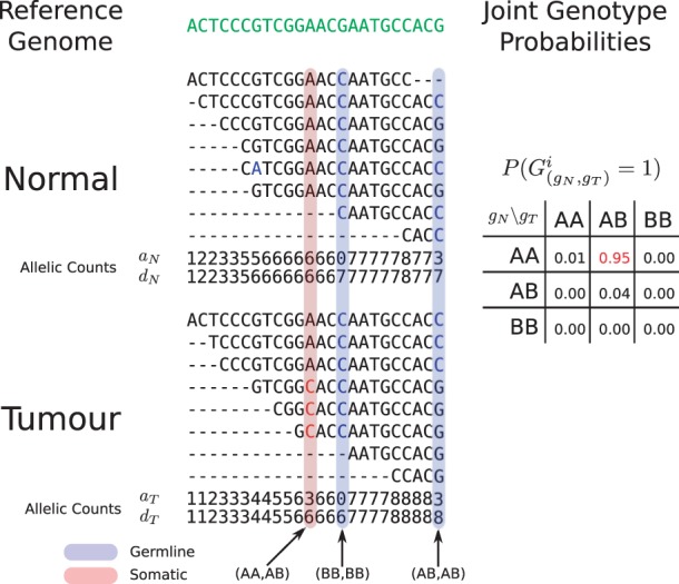
Hypothetical example of the JointSNVMix analysis process. Reads are first aligned to the reference genome (green). Next the allelic counts, which are the number of matches and depth of reads at each position are tabulated. Allelic count information can then be used to identify germline (blue) and somatic positions (red). At the bottom of the Figure, we show the hypothetical probabilities of the nine joint genotypes based on the count data for the somatic position (AA, AB).

For a diploid genome, we consider all pairs of alleles that gives rise to the set, ={AA, AB, BB}, the set of diploid genotypes. Now given two diploid samples, the set of possible joint-genotypes consists of all combinations of diploid genotypes, which is equivalent to the Cartesian product of with itself, i.e. ×={(g_N, g_T):g_N, g_T∈}.

We assume the joint genotype of a given position can be mapped onto the more biologically interpretable set of marginal genotypes according to Table 1. This can be done by assigning the joint genotype to the most probable state, or marginalizing together the joint genotype probabilities for a given state. As an example of marginalization, we compute ℙ(Somatic)=ℙ((AA, AB))+ℙ((AA, BB)), i.e. the sum of probabilities of a wild-type genotype in the normal data and a variant genotype in the tumour data.

Table 1.

The nine possible joint genotypes and their associated mappings onto biologically interpretable marginal genotypes

gN\gT	AA	AB	BB
AA	Wild-type	Somatic	Somatic
AB	LOH	Germline	LOH
BB	Errora	Error	Germline

Wild-type [no change: ℙ(AA, AA)], Somatic [wild-type normal and variant tumour: ℙ(AA, AB)+ℙ(AA, BB)], Germline [variant normal and tumour: ℙ(AB, AB)+ℙ(BB, BB)] and loss of heterozygosity [LOH–heterozygous normal and homozygous tumour: ℙ(AB, AA)+ℙ(AB, BB)].

^aWe treat the joint genotypes (BB, AB) and (BB, AA) as errors since this would imply that a homozygous variant mutates back to the reference base, which is a possible, but unlikely event. It is more plausible that these cases are simply errors due to alignment or base calling.

2.2 JointSNVMix models

JointSNVMix1 and JointSNVMix2 are generative probabilistic models that describe the joint emission of the allelic count data observed at position i in the normal and tumour samples. Figure 2 shows the graphical models representing JointSNVMix1 and JointSNVMix2. A complete description of the notation and model parameters is given in Table 2.

Fig. 2.

Probabilistic graphical model representing the (a) JointSNVMix1 and (b) JointSNVMix2 model. Shaded nodes represent observed values or fixed values, while the values of unshaded nodes are learned using EM. Only the distributions for the normal are shown below, the tumour distributions are the same. We have defined f(q|a, z)=z[qa+(1 − q)(1 − a)]+0.5(1 − z) and g(r|z)=zr+(1 − z)(1 − r). Description of all random variables is given in Table 2.

Table 2.

Parameters in the model are learned using the EM algorithm as discussed below, while hyper-parameters are fixed to the value given

Parameter	Description	Value
δ	Pseudo counts in Dirichlet prior on π	gN\gT	AA	AB	BB
		AA	1e5	1e2	1e2
		AB	1e2	1e3	1e2
		BB	1e1	1e1	1e3
π	Multinomial distribution over joint genotypes	Estimated by EM (M-step)
Gi	Genotype at position i	Estimated by EM (E-step)
axi	Number of bases matching the reference genome at position i in genome x∈{N, T}	Observed (JointSNVMix1 only)
ax:jxi	Indicator that base jx at position i matches reference in genome x∈{N, T}	Latent (JointSNVMix2 only)
zx:jxi	Indicator that base jx at position i is correctly aligned x∈{N, T}	Latent (JointSNVMix2 only)
dxi	Depth of coverage at position i in genome x∈{N, T}	Observed
qx:jxi	Probability that base call is correct in genome x∈{N, T}	Observed (JointSNVMix2 only)
rx:jxi	Probability that alignment is correct in genome x∈{N, T}	Observed (JointSNVMix2 only)
μx:gx	Parameter of Binomial distribution for genotype gx in genome x∈{N, T}	Estimated by EM (M-step)
αx:gx	α parameter in Beta prior distribution on μx:gx		AA	AB	BB
		Normal	1000	500	2
		Tumour	1000	500	2
βx:gx	β parameter in Beta prior distribution on μx:gx		AA	AB	BB
		Normal	2	500	1000
		Tumour	2	500	1000

We introduce a random variable Gⁱ as a Multinomial indicator vector representing the joint genotype of the samples. More explicitly Gⁱ=(G_(AA,AA)ⁱ, G_(AA,AB)ⁱ,…, G_(BB,BB)ⁱ) where G_(gN,gT)ⁱ=1 if the joint genotype of position i is (g_N, g_T), and G_(gN,gT)ⁱ=0 otherwise. We assume the count data from the two samples are jointly emitted from Gⁱ thus capturing correlations between the variables, and allowing statistical strength to be borrowed across the samples. This is the key insight that differentiates this model from running an independent analysis of each sample and joining the inferred genotypes post hoc.

Given the joint genotype of the sample, we model the normal and tumour sample as being conditionally independent. For JointSNVMix1, the conditional distribution for each sample is modelled as a three component mixture of Binomial densities, where the densities correspond to the genotypes AA, AB, BB. These conditional densities are the same as used by SNVMix1 model (Goya et al., 2010). For JointSNVMix2, the conditional densities are the same as SNVMix2 (Goya et al., 2010), which allows for the incorporation of base and mapping quality information. A complete description of the model is available in the Supplementary Material.

2.3 Inference and parameter estimation

We use the expectation maximisation (EM) algorithm to perform maximum a posteriori (MAP) estimation of the values of the model parameters and latent variables. One could hand-set parameters of the model to intuitive values; however, we expect that fitting the model will allow for sample-specific adjustments to inter-experimental technical variability and inter-sample variation from tumour–normal admixture (so called tumour cellularity) in the tumour samples. A full derivation of the update equations for JointSNVMix1 and JointSNVMix2 is given in the Supplementary Material.

We initialize training with user supplied parameter values. Local minima are a potential pitfall when training with EM. To check the models sensitivity to initial parameter values, we generated 100 sets of random parameters and started training from these parameters. We observed that the trained parameters consistently converge to the same values, suggesting local optima are not a major problem for this model (Supplementary Figs S2 and S3).

Storing the posterior marginals generated in the E-step requires (n) memory, thus for a large dataset training may exhaust available memory. To circumvent this problem, we subsample every n-th position with coverage exceeding a specified threshold in both the tumour and normal. For the results presented below, we subsampled every 100-th position with a coverage of at least 10 reads. Lower values of n and hence larger subsample sizes will lead to improved parameter estimates at the cost of using more memory and CPU time.

2.4 Implementation and performance

The JointSNVMix software package is implemented using the Python programming language with computationally intensive portions written in Cython. The input is aligned sequence data in base space stored in the SAM/BAM format (Li et al., 2009) from a tumour–normal pair. The program implements two main commands, train and classify. A typical analysis consists of training to learn the model parameters. These can then be used with the classify command. Doing both steps of the analysis using coding space positions from a 30× genome takes ∼6 h on a four core Intel i7 processor running at 1.73 GHz with 8 GB memory.

2.5 Datasets

Synthetic data: we generated the synthetic data by sampling 10⁶ sites from the JointSNVMix1 model in Figure 2a. We used the following parameters:

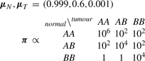π is normalized so that the sum over all entries equals 1. The depths d_Nⁱ, d_Tⁱ were sampled for a Poisson distribution with parameter λ=10. The synthetic data along with class labels is available in Supplementary Material.

We set parameters for the AB class in the vectors μ_N, μ_T to 0.6, which is slightly skewed towards the reference allele. We did this to ensure the parameters would be different than the hand-set defaults used in the untrained version of JointSNVMix1 and SNVMix1.

For the SNVMix1 and JointSNVMix1 models, we used a threshold ℙ(Somatic)≥0.5 to call mutations somatic in this experiment. We did not benchmark SNVMix2 and JointSNVMix2 because our simulation technique does not generate quality scores.

DLBCL: we analysed matched tumour/normal data from Morin et al. (2011) (dbGAP study accession phs000235.v2.p1). Exome data for patients A and B was captured using Agilent SureSelect, and subsequently sequenced on the Illumina GA II platform and aligned with Burrows-Wheeler Aligner (BWA). For patients C-M, the data were generated by whole genome shotgun sequencing (WGSS) and was run on the Illumina Hiseq2000 platform and aligned with BWA as described in Morin et al. (2011).

Ground truth data was predicted from the primary tumour genome and RNA-Seq data with the SNVMix software package followed by manual curation to remove artefacts. Support on both strands was required and variants near gapped alignments disregarded. Two or more high-quality bases matching SNV were required. Finally, putative variants were visually inspected in IGV. Validation of the non-synonymous curated predictions by targeted Sanger sequencing of the normal and tumour samples was performed to establish the true somatic mutations. There were 312 unique positions validated as somatic mutations across all patients in this study. Complete details are available in Morin et al. (2011).

In the analysis presented below, only coding space positions were analysed. For SNVMix2 and JointSNVMix2, no pre-processing was performed. For the other models, we removed bases with base or mapping qualities <10. Summary statistics for the aligned data are included in the Supplementary Material.

2.6 Alternative methods

In order to evaluate the effect of modelling the joint distribution of the tumour and normal data, we compared the JointSNVMix1 and JointSNVMix2 models to their independent analogues, SNVMix1 and SNVMix2. We re-implemented the SNVMix models in order to compare classifier performance without introducing variation due to implementation. We also considered independent and joint methods for classification which use Fisher's exact test. We include these two methods to verify the performance difference we observe in the SNVMix models are due to joint analysis.

Independent Fisher: this method uses a right-tailed Fisher's exact test in order to test the null hypothesis that the number of variant bases observed is due to random error. If the null hypothesis is not rejected at P-value of 0.05, the site is assigned the genotype AA. Otherwise, a site is assigned a genotype AB if the frequency of the B-allele is between 0.2 and 0.8, and a genotype of BB if this frequency is >0.8.

Joint Fisher: this method first applies the Fisher method to call the genotypes in normal and tumour separately. Putative somatic sites are identified and a two-tailed Fisher's exact test is run to test the null hypothesis that the normal and tumour count data do not differ significantly. If the null hypothesis is not rejected at P-value of 0.05, the putative somatic site is reassigned the reference genotype (AA,AA).

SNVMix1: we re-implemented the SNVMix1 model used in the published SNVMix software (Goya et al., 2010). To assign joint genotype probabilities, we take the genotype probabilities from the normal and tumour samples and multiply them to obtain the joint genotype probabilities.

SNVMix2: we re-implemented the SNVMix2 model used in the published SNVMix software (Goya et al., 2010). Joint genotype probabilities are derived as for SNVMix1.

2.7 Performance metrics

Since exhaustive validation of both somatic and non-somatic events was not available for the datasets used, we measured the concordance of the somatic predictions with databases known to be enriched for somatic or germline mutations. In theory, classifiers that predict more true somatic mutations should show higher concordance with the database of somatic mutations and lower concordance with the germline database.

To generate a database of somatic mutations, we took the complete set of 312 unique somatic mutations validated across the cases and joined them with COSMIC v54 database (Forbes et al., 2011). We used the SNP predictions from the 2010/11/23 release of the 1000 genomes projects (Durbin et al., 2010), with the positions found in COSMIC v54 removed, as the database of likely germline variants.

For the SNVMix and JointSNVMix methods, which assign probabilities to their predictions, we plot curves based on the rank ordering of somatic predictions. We do this by computing concordance as the probability threshold for classification is lowered. For the Fisher methods, which do not assign scores to their predictions, we plot a point in space for the complete set of predictions.

To estimate the recall rate of the JointSNVMix models, we computed how many of the validated mutations for a case were found by the models using a threshold of ℙ(Somatic)≥0.5. There were 307 validated positions across the 12 cases used for this analysis. This number differs from the 312 unique positions because some mutations are found across multiples cases, and some cases from the original study were not included in our analysis.

We note that copy number variation (CNV) due to segmental aneuploides and abnormal karyotypes could affect predictions. To assess the effect of CNV on prediction accuracy, we repeated the recall experiment using positions found in regions of predicted CNVs. CNVs were predicted (Supplementary Fig. S4) using an in-house tool, HMMCopy, available from http://compbio.bccrc.ca. This tool requires whole genome data, so patients A and B had to be excluded from this analysis. When we excluded these cases there were 187 validated somatic positions, 44 (23.5%) of which were found in regions of CNV.

3 RESULTS

3.1 Joint modelling shows increased ability to detect shared signals on simulated data

We summarize the results from our synthetic experiment in Table 3. The F-measure and Matthews correlation coefficient (MCC) for the trained JointSNVMix1 model is the highest among all models, reflecting a good trade-off between sensitivity and specificity. The trained SNVMix1 model had the most true positives of all models; however, the F-measure and MCC were lower than JointSNVMix1. This is due to the high number of false positives (823) associated with the method, the bulk of which are false positive germline events (743).

Table 3.

Results from synthetic data

Caller	TP	FP	TN	FN	F-meas	MCC	FP Germlines	FP Wild-types
JointSNVMix1 (Trained)	140	13	999788	59	0.795	0.802	8	2
JointSNVMix1	153	50	999751	46	0.761	0.761	42	0
SNVMix1 (Trained)	190	823	998978	9	0.314	0.423	743	70
Joint Fisher	159	1155	998646	40	0.21	0.311	1109	0
SNVMix1	178	1653	998148	21	0.175	0.295	1632	0
Independent Fisher	159	2538	997263	40	0.11	0.217	2464	0

We report the number of true positives (TP), false positives (FP), true negatives (TN), false negatives (FN), F-measure (F-meas), Matthews correlation coefficients (MCC), false positives which are germline (FP Germlines), and false positives which are wild-type (FP Wild-types). The best results for each category are shown in bold.

There is an obvious bias associated with simulating from the JointSNVMix1 model to generate the synthetic data. We only present this data to emphasize the relatively high false positive rate that can be expected from post hoc methods, which treat the data as being independently sampled. When comparing number of false positives for JointSNVMix1 and SNVMix1, we observed an 80-fold reduction with the joint modelling approach. This trend is supported by the Fisher models where we see a 2-fold reduction in false positives when using the joint approach.

3.2 Joint modelling increases enrichment of true somatics in high ranking predictions

In Figure 3, we show the aggregated concordance analysis results for the 12 DLBCL cases. (Supplementary Fig. S1 shows concordance results for each case separately.) The circles at the start of the lines for the JointSNVMix and SNVMix models represents the set of predictions for which ℙ(Somatic)=1. The JointSNVMix models show higher somatic concordance (left) in the top mutations predicted, while showing lower germline concordance (right) than their SNVMix analogues. This suggests that by distinguishing and removing false positive germline events, JointSNVMix enriches the top ranked somatic predictions for true somatic mutations.

Fig. 3.

Concordance analysis of the 12 DLBCL datasets. The Somatic column represents concordance with the merged COSMIC and ground truth set. The germline column represents concordance with the 1000 Genomes positions with the cosmic positions removed. The horizontal axis shows the number of somatic predictions made and the vertical axes shows the fraction of those predictions found to be in the respective set. Lines are drawn by computing concordance as the threshold for classification is lowered. Lines start always from the left side because multiple positions may have ℙ(Somatic)=1. Circles at the start of lines indicate this positions, these points are also labelled with the number of somatic predictions (in 1000's) and concordance.

Comparing the Fisher methods, we see that the joint model significantly improves performance. The independent Fisher method produces an unrealistically large number of predictions; however, the joint Fisher approach seems much better. A major limitation of the Fisher methods is the lack of ranking information. As a result, we can only compare these methods to JointSNVMix and SNVMix models at a single point. At this single point, the Fisher methods have similar somatic concordance, but higher germline concordance. This suggests that the sensitivity of the Fisher methods is similar to the SNVMix family of models, but the specificity is lower.

JointSNVMix2 has a recall rate of 0.935 (287/307) on the validated mutations, which is higher than JointSNVMix1's rate of 0.915 (281/307). JointSNVMix2 shows similar or higher somatic and germline concordance than JointSNVMix1 model. This suggests that JointSNVMix2 is erring on the side of recall versus specificity when compared with JointSNVMix1, though the performance is not dramatically different. One benefit of the JointSNVMix2 model as previously discussed in Goya et al. (2010), is that it frees the user from setting arbitrary thresholds on base and mapping quality.

The recall rates for both JointSNVMix1 and 2 was 0.864 (38/44) in regions of CNV, while in copy neutral regions recall rates were 0.916 (131/143) and 0.923 (132/143). This suggests that CNV slightly degrades the performance of both methods, although neither method showed statistically worse performance (Fisher's exact test, P=0.3787, P=0.2383, respectively.)

In total, there were 2496 somatic variants called by JointSNVMix2 at the highest stringency (P=1) of which 559 were non-synonymous variants not present in 1000 genomes polymorphism database. As discussed earlier, Morin et al. (2011) used stringent criteria, manual curation and validation to establish the 307 true mutations. We did not validate the non-intersecting predictions in this contribution, leaving the possibility of false positive events due to technical artefacts. We suggest a robust solution to mitigate against technical artefacts in Section 4.

4 DISCUSSION

In this article, we examined the problem of simultaneous analysis of tumour–normal pair NGS data for the purpose of identifying somatic point mutations. We developed a probabilistic framework called JointSNVMix to allow us to benchmark a model that can borrow statistical strength between samples against standard independent analysis. We showed that joint modelling of genotypes confers an increased specificity over simpler or independent analysis (Section 3.2). Interestingly, the frequentist statistics-based method, ‘joint Fisher’ method, which considers both datasets simultaneously shows an increased specificity over its ‘independent’ analogue, albeit considerably lower than what was achieved for JointSNVMix.

4.1 Limitations and extensions

Data preprocessing: in our study, we assume that the input data is aligned correctly and focus specifically on the problem of identifying somatic mutations from allelic counts extracted from perfectly aligned data. The scope of this study is thus restricted to examining the effects of model-based classifiers for identifying somatic mutations from count-based data. The alignment and pre-processing steps leading to the generation of the count data are expected to have a dramatic effect on the quality of the classifiers we considered. The simple approach we used of filtering (JointSNVMix1) or modelling (JointSNVMix2) mapping and base qualities is likely suboptimal since they both do not consider technical artefacts such as strand bias. However, all classifiers are presented with the same data, and all will likely benefit to the same degree from improved pre-processing. As our software makes use of BAM files as inputs, it is agnostic to any upstream processing in the generation of these files, and as such should be compatible with more sophisticated pre-processing strategies and efforts such as Samtools and GATK will likely continually improve this important aspect of analysis. In our experience, post-processing JointSNVMix predictions with mutationSeq (Ding et al., 2012) removes the majority of technical artefacts.

Model extensions: the JointSNVMix models make several simplifying assumptions that may negatively affect performance. In future work, it would be interesting to extend the framework presented here to model tumour–normal admixture, aneuploidy, CNV and nucleotide identity. We note in Section 3.2 that although ∼25% of mutations fell in regions of CNV, sensitivity was not significantly affected when copy neutral mutations and mutations in regions of CNV were compared. The effect of substantially altered karyotypes (typically exhibited by epithelial malignancies) on the ability to detect somatic mutations remains an open question. However, we expect that explicit modelling of the genomic complexities of cancer such as CNVs and subclonal populations would lead to enhanced interpretability of somatic mutation prediction and enhanced performance. In addition, the iid nature of the model easily allows for location-specific prior knowledge of germline polymorphisms to be incorporated into the joint genotype prior. As population-level databases mature, this extension to the model should increase the specificity of somatic mutation predictions.

5 CONCLUSIONS

In this article, we formulated the joint genotype problem for somatic mutation discovery from a tumour–normal pair of NGS datasets. We have developed a novel statistical model JointSNVMix, which explicitly models the process that jointly generates a pair of samples. The joint modelling approach employed JointSNVMix allows us to reduce the number of germline events falsely predicted to be somatic. This increased specificity comes with little to no decrease in sensitivity.

Additionally, we have provided a complete software package for detecting somatic mutations in paired sequence data. This package includes not only the JointSNVMix1/2 classifiers, but the other four methods presented in the article. The Python implementation of our software is available under an open-source license from http://compbio.bccrc.ca.

Funding: Canadian Institutes for Health Research (CIHR) grant #202452. A.R. is supported by the CIHR. S.P.S. is supported by the Canadian Breast Cancer Foundation and the Michael Smith Foundation for Health Research.

Conflict of Interest: none declared.

REFERENCES

- Berger M.F., et al. The genomic complexity of primary human prostate cancer. Nature. 2011;470:214–220. doi: 10.1038/nature09744. [DOI] [PMC free article] [PubMed] [Google Scholar]
- Campbell P.J., et al. The patterns and dynamics of genomic instability in metastatic pancreatic cancer. Nature. 2010;467:1109–1113. doi: 10.1038/nature09460. [DOI] [PMC free article] [PubMed] [Google Scholar]
- DePristo M., et al. A framework for variation discovery and genotyping using next-generation DNA sequencing data. Nat. Genet. 2011;43:491–498. doi: 10.1038/ng.806. [DOI] [PMC free article] [PubMed] [Google Scholar]
- Ding L., et al. Genome remodelling in a basal-like breast cancer metastasis and xenograft. Nature. 2010;464:999–1005. doi: 10.1038/nature08989. [DOI] [PMC free article] [PubMed] [Google Scholar]
- Ding J., et al. Feature based classifiers for somatic mutation detection in tumour-normal paired sequencing data. Bioinformatics. 2012;28:167–175. doi: 10.1093/bioinformatics/btr629. [DOI] [PMC free article] [PubMed] [Google Scholar]
- Durbin R.M., et al. A map of human genome variation from population-scale sequencing. Nature. 2010;467:1061–1073. doi: 10.1038/nature09534. [DOI] [PMC free article] [PubMed] [Google Scholar]
- Forbes S.A., et al. COSMIC: mining complete cancer genomes in the Catalogue of Somatic Mutations in Cancer. Nucleic Acids Res. 2011;39:D945–D950. doi: 10.1093/nar/gkq929. [DOI] [PMC free article] [PubMed] [Google Scholar]
- Goya R., et al. SNVMix: predicting single nucleotide variants from next-generation sequencing of tumors. Bioinformatics. 2010;26:730–736. doi: 10.1093/bioinformatics/btq040. [DOI] [PMC free article] [PubMed] [Google Scholar]
- Hudson T., et al. International network of cancer genome projects. Nature. 2010;464:993–998. doi: 10.1038/nature08987. [DOI] [PMC free article] [PubMed] [Google Scholar]
- Jones S.J., et al. Evolution of an adenocarcinoma in response to selection by targeted kinase inhibitors. Genome Biol. 2010;11:R82. doi: 10.1186/gb-2010-11-8-r82. [DOI] [PMC free article] [PubMed] [Google Scholar]
- Koboldt D.C., et al. VarScan: variant detection in massively parallel sequencing of individual and pooled samples. Bioinformatics. 2009;25:2283–2285. doi: 10.1093/bioinformatics/btp373. [DOI] [PMC free article] [PubMed] [Google Scholar]
- Larson D., et al. SomaticSniper: identification of somatic point mutations in whole genome sequencing data. Bioinformatics. 2012;28:311–317. doi: 10.1093/bioinformatics/btr665. [DOI] [PMC free article] [PubMed] [Google Scholar]
- Ley T.J., et al. DNA sequencing of a cytogenetically normal acute myeloid leukaemia genome. Nature. 2008;456:66–72. doi: 10.1038/nature07485. [DOI] [PMC free article] [PubMed] [Google Scholar]
- Li H., et al. The sequence alignment/map format and SAMtools. Bioinformatics. 2009;25:2078. doi: 10.1093/bioinformatics/btp352. [DOI] [PMC free article] [PubMed] [Google Scholar]
- Mardis E.R. Cancer genomics identifies determinants of tumor biology. Genome Biol. 2010;11:211. doi: 10.1186/gb-2010-11-5-211. [DOI] [PMC free article] [PubMed] [Google Scholar]
- Mardis E.R., et al. Cancer genome sequencing: a review. Hum. Mol. Genet. 2009;18:R163–R168. doi: 10.1093/hmg/ddp396. [DOI] [PMC free article] [PubMed] [Google Scholar]
- McKenna A., et al. The Genome Analysis Toolkit: a MapReduce framework for analyzing next-generation DNA sequencing data. Genome Res. 2010;20:1297. doi: 10.1101/gr.107524.110. [DOI] [PMC free article] [PubMed] [Google Scholar]
- McLendon R., et al. Comprehensive genomic characterization defines human glioblastoma genes and core pathways. Nature. 2008;455:1061–1068. doi: 10.1038/nature07385. [DOI] [PMC free article] [PubMed] [Google Scholar]
- Morin R., et al. Frequent mutation of histone-modifying genes in non-Hodgkin lymphoma. Nature. 2011;476:298–303. doi: 10.1038/nature10351. [DOI] [PMC free article] [PubMed] [Google Scholar]
- Morin R.D., et al. Somatic mutations altering EZH2 (Tyr641) in follicular and diffuse large B-cell lymphomas of germinal-center origin. Nat. Genet. 2010;42:181–185. doi: 10.1038/ng.518. [DOI] [PMC free article] [PubMed] [Google Scholar]
- Pleasance E., et al. A comprehensive catalogue of somatic mutations from a human cancer genome. Nature. 2009a;463:191–196. doi: 10.1038/nature08658. [DOI] [PMC free article] [PubMed] [Google Scholar]
- Pleasance E., et al. A small-cell lung cancer genome with complex signatures of tobacco exposure. Nature. 2009b;463:184–190. doi: 10.1038/nature08629. [DOI] [PMC free article] [PubMed] [Google Scholar]
- Shah S.P., et al. Mutation of FOXL2 in granulosa-cell tumors of the ovary. N. Engl. J. Med. 2009a;360:2719–2729. doi: 10.1056/NEJMoa0902542. [DOI] [PubMed] [Google Scholar]
- Shah S.P., et al. Mutational evolution in a lobular breast tumour profiled at single nucleotide resolution. Nature. 2009b;461:809–813. doi: 10.1038/nature08489. [DOI] [PubMed] [Google Scholar]
- Sherry S., et al. dbSNP: the NCBI database of genetic variation. Nucleic Acids Res. 2001;29:308. doi: 10.1093/nar/29.1.308. [DOI] [PMC free article] [PubMed] [Google Scholar]
- Wiegand K.C., et al. ARID1A mutations in endometriosis-associated ovarian carcinomas. N. Engl. J. Med. 2010;363:1532–1543. doi: 10.1056/NEJMoa1008433. [DOI] [PMC free article] [PubMed] [Google Scholar]
- Yachida S., et al. Distant metastasis occurs late during the genetic evolution of pancreatic cancer. Nature. 2010;467:1114–1117. doi: 10.1038/nature09515. [DOI] [PMC free article] [PubMed] [Google Scholar]
Associated Data
This section collects any data citations, data availability statements, or supplementary materials included in this article.