Review of Fast Monte Carlo Codes for Dose Calculation in Radiation Therapy Treatment Planning

Abstract

An important requirement in radiation therapy is a fast and accurate treatment planning system. This system, using computed tomography (CT) data, direction, and characteristics of the beam, calculates the dose at all points of the patient's volume. The two main factors in treatment planning system are accuracy and speed. According to these factors, various generations of treatment planning systems are developed. This article is a review of the Fast Monte Carlo treatment planning algorithms, which are accurate and fast at the same time. The Monte Carlo techniques are based on the transport of each individual particle (e.g., photon or electron) in the tissue. The transport of the particle is done using the physics of the interaction of the particles with matter. Other techniques transport the particles as a group. For a typical dose calculation in radiation therapy the code has to transport several millions particles, which take a few hours, therefore, the Monte Carlo techniques are accurate, but slow for clinical use. In recent years, with the development of the ‘fast’ Monte Carlo systems, one is able to perform dose calculation in a reasonable time for clinical use. The acceptable time for dose calculation is in the range of one minute. There is currently a growing interest in the fast Monte Carlo treatment planning systems and there are many commercial treatment planning systems that perform dose calculation in radiation therapy based on the Monte Carlo technique.

INTRODUCTION

Radiation therapy is the use of high-energy particles or rays to damage cancer cells and prevent them from growing. This treatment modality can be used alone or in conjunction with surgery, chemotherapy or hormonal therapy to treat cancer. The source of radiation could be X-rays, gamma rays, electrons, neutrons, protons, and so on. The goal of radiation therapy is to damage as many cancer cells as possible, while limiting harm to the nearby healthy tissue and irradiating a minimal dose in the critical organs.[1]

In the treatment planning stage, using all available information, including that obtained from the simulation, the final plan will determine the technique, type of therapy, size, the number of X-ray beams, and the direction of each beam. Next, using the role of the physics of radiation therapy in the treatment planning software, the dose and various voxels of the CT scan are calculated. Each voxel in the CT corresponds to a point in the patient. Finally, the dose distribution is illustrated for evaluation of the treatment. This illustration is usually in the form of isodose lines. Isodose lines are the lines through the points, with the same amount of dose.

There are several methods for dose calculation in radiation therapy, such as, the pencil beam algorithm,[2] superposition-convolution algorithm,[3] and the Monte Carlo techniques.[4] In the pencil beam algorithm, an electron beam is modeled as a collection of forward-directed ‘pencils’ after the collimation device of the accelerator. The electron pencil beams at subsequent planes are redistributed in a Gaussian distribution due the scatter in the medium and air.

In the superposition-convolution algorithm the ‘total energy released per unit mass’ is convolved with the ‘energy deposition kernels’[5] generated in the homogeneous media of different densities, to obtain the dose distribution.

The Monte Carlo (MC) method is a statistical simulation method based on random sampling.[4] For radiation transport problems, this technique simulates the tracks of individual particles by sampling appropriate quantities from the probability distributions governing the individual physical processes, using machine-generated random numbers.

The MC technique is the most accurate method for radiotherapy treatment planning dose calculation, which is capable, in principle, of accurately computing the dose under almost all circumstances. Extensive efforts have been made to improve the MC dose calculation algorithms used in the treatment planning systems to accurately reproduce all beam geometries and beam modification devices and to account for the effects of heterogeneities in the full three-dimensional (3D) patient geometry.

MONTE CARLO TECHNIQUE

The Monte Carlo (MC) methods are stochastic techniques that are based on the use of random numbers and probability statistics, to investigate problems.[6] Thus, the MC methods are a collection of different methods that perform the same process: This process involves performing many simulations using random numbers and probability distributions to get an approximation of the answer to the problem. The defining characteristic of the MC methods is its use of random numbers throughout the simulation process. One of the most important usages of the MC methods is in the evaluation of difficult integrals such as multi-dimensional integrals.[7]

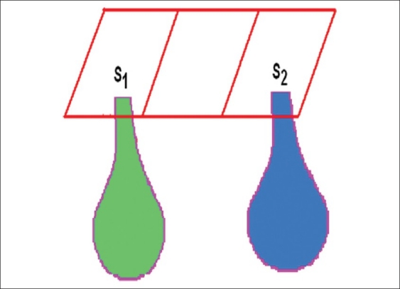
An example of a MC technique is illustrated in Figure 1 In this example, the area s₂, with an irregular shape, is to be calculated. First, we place the area s₂ inside a regular (rectangular) shape s₁, the area of which is known. Subsequently, we cover the s₂ with many (n₁) randomly distributed dots and we count the number of dots that hit s₂. The ratio of the two numbers is proportional to the ratio of the surfaces:

Figure 1.

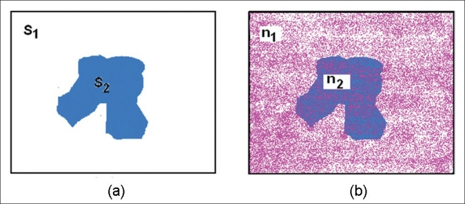
An example of Monte Carlo technique for area calculation of an irregular shape

There are two requirements to have an acceptable answer:

1. The number of the points has to be large so that the ratio of the numbers approaches the ratio of the areas

2. The points have to be distributed randomly to avoid a systematic error

The obligation of having a large number of points (or simulations for other types of the problems) generally makes the Monte Carlo method a slow technique.

MONTE CARLO IN RADIATION THERAPY

The Monte Carlo techniques have been used in various branches of radiation therapy,[8,9] from simulation of radiation therapy equipments and sources to dose calculation in various geometries.[10–18] For simulation of the photon and electron particles one has to apply the physics of transport for modeling, which requires the knowledge of interactions of the particle, probability of each interaction, and other information. When an electron traverses matter, it interacts with the electrons and the nuclei of the medium and begins to lose energy as it penetrates the medium.

The interaction can be generally categorized as collisions between the electron and either the atomic electrons or the nucleus.[19] The collisions are described as soft and hard collisions. In soft collisions, the electron passes an atom at a relatively large distance, and the Coulomb force field affects the whole atom with an excitation or ionization. In this kind of collision, a small amount of energy can be transferred to the medium. A hard collision is the interaction of the particle with a single bound electron, which leads to the ionization of the atoms in the matter, in which knock-on electrons (or δ-rays) are produced.

An electron, in reality, undergoes a very large number of elastic and inelastic interactions and it is not possible to simulate each electron collision explicitly. Therefore, in MC calculations, inelastic collisions are grouped into a discrete process, with continuous energy loss (condensed history simulation, Figure 2).[8] In a discrete process (hard collisions) secondary particles are produced with an energy above a user defined threshold. The energy of the electrons is supposed to be deposited in the surrounding medium continuously between the hard collisions [Figure 2a and b]. The elastic collisions are described by changes in the direction of movement after each electron step.

Figure 2.

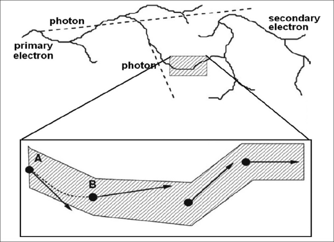
Illustration of the condensed history algorithm. The track of the electron (above) includes many secondary electrons and photons (dashed line in the upper panel). The electron track in the shaded box is simulated with a condensed history algorithm. The initial and final positions of the electron in one step are A and B, which include the scattering of the electron in the medium. However, condensed history implementation does not provide information on how the particle goes from A to B. The curved dashed line connecting A and B is a more realistic representation of the trajectory than a straight line from A to B. (Figure modified from Ref.[8])

The particles in the MC calculations are transported until they reach a user defined energy cut-off (e.g., 0.01 MeV for photons and 0.6 MeV for electrons). Through a large number of simulations (histories) the quantity of interest can be calculated, for example, the deposited energy in each voxel.

As for the statistical nature of MC calculations, each calculated parameter is subject to a statistical uncertainty and one can reduce the uncertainty with a larger number of histories or many variance reduction techniques.[20–23] Variance reduction techniques reduce the time for particle simulations and improve the speed of the code. These techniques (few of which are discussed in the following sections) are important elements of any MC code and may be different for various applications and geometries.

A general purpose MC code should consider all aspects of the electron and photon transport and it should be able to produce accurate results in a heterogeneous phantom. Several general purpose MC codes have been developed for radiation transport calculation, which are used in medicine, such as, EGS4,[24] EGSnrc,[25] MCNP,[26] and GEANT.[27] The MC codes for simulation of linear accelerators and dose calculation in the patient are BEAMnrc[28] and DOSXYZnrc,[29] which are based on EGS4/EGSnrc.

EGSnrc/BEAMnrc/DOSXYZnrc are some of the most widely used packages in radiation therapy.[9] EGSnrc is a version of the program Electron Gamma Shower 4 (EGS4) and has been applied to all areas of radiation protection, dosimetry, and medical physics, and has been extensively validated.[30–37] BEAMnrc is used to simulate many types of radiotherapy sources and clinical accelerators.[38–40] BEAMnrc can produce a phase-space output of the beam (including energy, charge, position, and direction) at any specified plain in geometry. DOSXYZnrc is designed for dose calculations in 3D rectilinear voxel geometry. The output data calculated by BEAMnrc can be used as an input file for DOSXYZnrc. All three codes (EGSnrc/BEAMnrc/DOSXYZnrc) can run under the UNIX or Windows Operating Systems.[41]

The simulation of a linear accelerator with BEAMnrc is combined with DOSXYZnrc, in which a CT data set can be used as an input file and simulation of each particular patient can be handled.

THE NEED FOR A FAST MONTE CARLO CODE

The general-purpose MC codes transport the particles in a wide range of energies and materials with the best available transport algorithms and cross-sections.[42] The general-purpose codes have been designed for all application types and have not been optimized for clinical situations. Hence, despite clever variance reduction techniques, they are relatively slow for dose calculations in the treatment planning systems.[43] Consequently in the past decade, several fast MC codes have been developed to improve the efficiency and decrease the calculation time, such as, Macro Monte Carlo,[44,45] Superposition Monte Carlo,[46,47] Voxel-based Monte Carlo (VMC, VMC++),[48–51] Dose Planning Method (DPM),[52] and MCDOSE.[53]

Although with the speed of recent computer hardware and using parallel processing techniques, it has become possible to run a general purpose code in a reasonable amount of time, fast MC techniques are still essential for applications such as a four-dimensional MC (Monte Carlo for moving components).[54–57] All the mentioned fast MC codes benchmark their results to the EGS4 or the EGSnrc code and the gain of speed has been 10–50 times faster for electron transport. Most of the fast MC codes have been improved from their original versions over the past few years; they have also been compared with benchmark experiments and produce mostly accurate results.[58–67] MMC, SMC, and VMC++ have reached speed up factors 20, 30, and 50 times faster than EGS4, respectively, and their dose distributions are typically within 3–4, 2, and 1% of the EGS4 results, respectively. The details of different approaches for a fast MC are discussed in the following sections.

MACRO MONTE CARLO

Sphere by Sphere Transport of the Electron

Macro Monte Carlo (MMC) is one of the very first fast MC codes that was developed in 1992.[44] At that time, the pencil beam algorithm was the most successful methods to calculate the electron beam dose in radiation therapy.[68,69] However, large differences between pencil beam calculations and experiments were reported.[70–72] The MC methods were also very slow with the available computers and the MMC code was developed to apply the MC techniques in a more efficient manner.

The MMC code transports the MMC in sphere-by-sphere macroscopic steps, as illustrated in Figure 3 The characteristics of the electron after each sphere are determined from the pre-calculated database. The resulting parameters of the electron after each step are sampled from a pre-calculated probability distribution.

Figure 3.

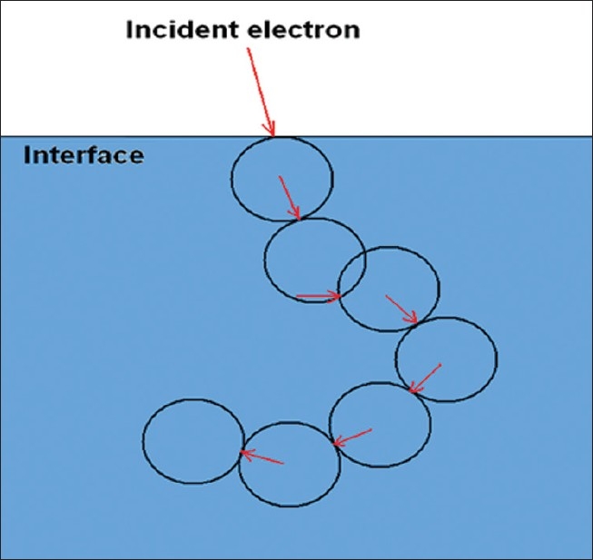
Electron transport in MMC. The direction of an electron after each spherical step is indicated by arrows and is determined by using per-calculated data

Generation of Probability Functions

Pre-calculated data are generated by EGS4, in which an electron is vertically incident on the surface of the macroscopic sphere. The geometry of the incident electron and the sphere is illustrated in Figure 4. The initial parameters for generation of pre-calculated data are the radius of the sphere, density and material of the sphere, and incident energy of the electron.

Figure 4.

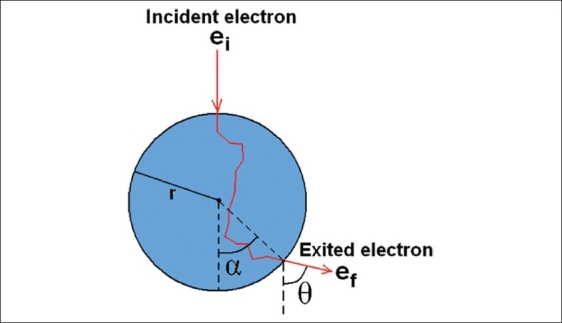
The geometry of the incident electron and various parameters used for the database of MMC

The radius of the sphere has a constant value of r=0.2 cm. Keeping the radius constant certainly produces some artifacts near the inhomogeneities, which will be discussed later. In this method, the sphere is like a black box, from which several secondary particles as well as primary electrons come out. The electron with the highest energy is considered the primary electron.

For various material and energies, the following parameters are stored in the database:

1. The distribution of the scattering angle (θ in Figure 4) and the angle of the exited primary electron (α). The α angle technically determines the exited position of the primary electrons, as the radius is known. The possible range of the angles is split up into 18 bins. In the stored set, the probability of emergence in each angular beam and the mean angles (θ ,α) are saved as a discrete cumulative density function.

2. Energy distribution of the exited primary electron (ef in Figure 4). The possible range of ef (which is from 0 to the energy of the primary electron) is divided in 20 bins and the probability of each bin is saved in a discrete cumulative energy function.

3. Probability of absorption of the primary electron in the sphere. This probability is calculated by dividing the number of exited primary electrons by the total number of incident primary electrons.

4. Probability that ‘transferred energy’ (e_i–e_f) is deposited in a sphere or transferred to a secondary electron or secondary photon.

5. A few other parameters that are required for complete transport of the particle are also saved. These include the range of the exited secondary electrons with Continuous Slowing Down Approximation (CSDA range). The secondary electrons in MMC are not transported explicitly and the energy is deposited according to CSDA approximation.

The pre-calculated data was generated for different materials such as lung (ρ=0.3 g/cm³), water (ρ=1 g/cm³), Lucite (ρ=1.19 g/cm³), solid bone phantom material (ρ=1.84 g/cm3), and aluminum (ρ=2.7 g/cm³). The energy cut-offs were set at 190 keV for electrons and 100 keV for photons. For each material the simulations were done using an energy range of 0.2–20 MeV (0.2, 0.4, 0.6, 0.8, 1, 1.5, 2, 3, …, 19, 20 MeV). For a statistical uncertainty of 1% in the primary electron parameters in MMC, 30000 electrons were simulated for each sphere (with various energies and materials).

Comparison of MMC Results with EGS4

An interesting illustration of the results for distribution of exited primary electrons on the surface of the sphere for various energies is illustrated in Figure 5. The length of the vectors is proportional to the number of electrons, and the results are illustrated for three sets of the incident parameters: water-8 MeV, water-1.5MeV, and bone-1.5 MeV. At high energies, the electrons emerge in the forward direction with a small scattering angle. On account of the larger scattering power of the bone, the emerged electrons are widely scattered in the orthogonal direction.

Figure 5.

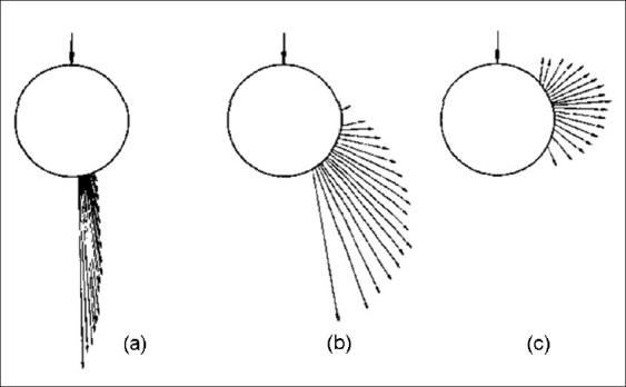
Spatial distributions of exited primary electrons on the surface of the sphere. (a) Water sphere, incident energy (ei)=8 MeV, (b) water sphere ei=1.5 MeV, (c) bone sphere ei=1.5 MeV (Figure from Ref.[44])

The results of MMC are compared to EGS4 with the same cut-off parameters. Figure 6a illustrates the depth-dose distribution for monoenergetic electron beams of various energies, incident normal to the surface of a water phantom. The data are collected on the central axis for a 20 cm×20 cm field and the differences between MMC and EGS4 are 2–4%. Figure 6b illustrates an example of MMC results in a heterogeneous medium in which a slab of bone and lung is embedded in a water phantom. The energy of the incident electron is 20 MeV and there are relatively large discrepancies of up to 8% near the interfaces. The MMC code is implemented in many clinical cases such as the head phantom, and the errors compared to EGS4 are in the range of 2–7%.

Figure 6.

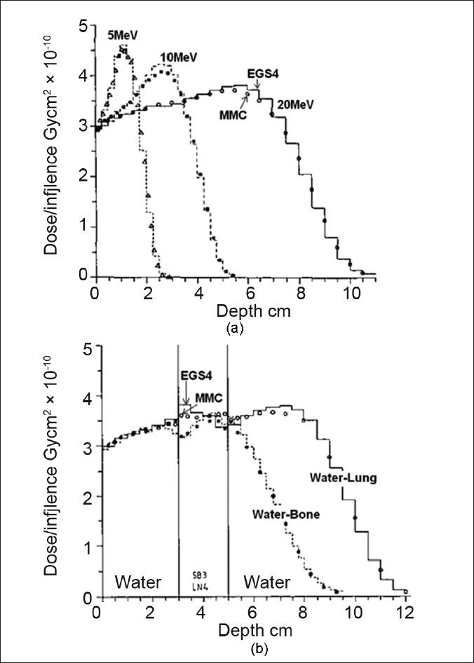
(a) Depth dose of central axis for various energies in the water phantom in comparison with EGS4. The field size of the electrons beams were 20×20 cm². (b) Central axis depth dose of 20 MeV electrons in water with a lung and bone slab (Figures modified from Ref.[44])

Discussion of MMC Results

The MMC generally has a large discrepancy in the buildup region of the dose distribution and near the interfaces of different materials. The errors are mainly due to several approximations for the transport of primary and secondary electrons. An approximation that produces large errors in the buildup region is due to the transport of the electrons in a straight path between the entrance and the exit point, as illustrated in Figure 7. In MMC, the path of the electrons is lost in pre-calculated spheres, although the real path of the electrons is a random path. This assumption particularly produces large errors for regions with large dose gradients, such as the buildup region. It is possible to reduce the size of the spheres in the pre-calculated data, however, the total size of the pre-calculated data will increase as a result.

Figure 7.

Transport of the electron in MMC in a voxel-based phantom. The energy of the electron is deposited in a straight line from the entrance to the exit point of the sphere

Other approximations that produce large errors are: (1) Constant radius of the sphere. An extension of the pre-calculated data for various size spheres increases the size of the pre-calculated data; however, it improves the accuracy of the results as will be discussed later. (2) Transport of the secondary electrons with CSDA approximation. (3) Approximation of angular distribution of the exited electrons in bin angles.

The above-mentioned approximations in MMC had been imposed by a limited available computer RAM at that time. The size of the pre-stored data in the MMC for each material was around 100 kb, which was also suitable for parallel processing. The speed factor of the MMC with respect to EGS4 was 4–10 for various geometries. MMC is commercially available for linear accelerators and the performance of the clinical implementation has been evaluated in the literature.[61,73]

Further Developments in MMC

As mentioned earlier, the early version of the MMC produced large artifacts in the buildup region and near the interfaces of different materials. In a follow-up development,[45] the original version of MMC was significantly modified, in order to increase the speed and address the relatively large errors of the code.

The constant size of the sphere was recognized as the major reason for the poor performance of the code near the interfaces.

The authors implemented a newly developed adaptive step size algorithm in which the size of the spheres depended on the distance of the electron from the interface. There were other features in the new version of the MMC which improved the results of the code, and these will be discussed in this section.

Adaptive step size algorithm: The original MMC database contained a single sphere size of r=0.2 cm. To develop an adaptive step size algorithm, the database had to be expanded to include data for different sphere sizes. In the new version, five different sphere sizes were used for the generation of pre-calculated data (0.05, 0.1, 0.15, 0.2, and 0.3 cm). The size of the spheres had to be smaller than 3 mm, as the larger size of the sphere produced large artifacts in the dose buildup region. The resulting MMC database required 200 kb of memory.

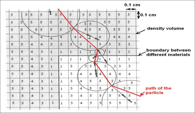
Pre-process of the absorber volume: To use various sphere sizes, at each step, the distance of the electron from the closest boundary should be calculated. This calculation in-the-fly is time consuming and an algorithm is developed that allows the determination of the sphere sizes and mean density in each voxel of the CT phantom, by pre-processing of the whole CT volume, prior to MMC simulation. For this purpose, first the CT volume is converted to a density volume with a user-defined resolution (0.1–0.2 cm) through the application of CT to density conversion factors.

In the second step, the resulting density volume is scanned for heterogeneities. A sphere size is assigned to each voxel, with a volume that corresponds to the maximum radius of the sphere that can be placed in the center of the voxel, without reaching into the other materials. This process results in small sphere sizes near the interfaces of different materials, and large spheres to the point, at a large distance from the interfaces. The interface is defined between the voxels in which the ratio of densities are larger than 1.5. An example of a pre-processed head phantom is illustrated in Figure 8. The importance of this technique is that a similar idea can also be used for fast transport of the particles in other MC codes.

Figure 8.

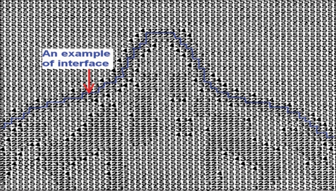
A pre-processed CT slice of the head. The resolution of the voxels are 2 mm in each direction. The numbers illustrate the sphere size that can be used for that voxel without crossing the interfaces. The number, two, is related to the smallest spheres size, 2 mm (Figure modified from Ref.[45])

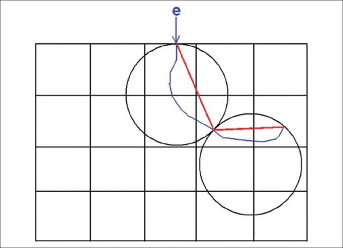
Transport algorithm: An illustration of an adaptive step size algorithm is shown in Figure 9. Using the pre-processed volume, the step size of the electron in each voxel is already available. The center of the sphere is placed at the distance of one radius of the maximum allowed sphere size in the current position of the electron. The direction of the motion is determined from the direction of the exited electron from the previous sphere.

Figure 9.

Transport of the electron using the adaptive step size algorithm. The arrows illustrate the direction of the exited primary electron and the straight line illustrates the path of the electron. The position of the spheres is determined by the number of the voxel (representing the size of the sphere) and direction of the emerged primary electron from the surface of the previous sphere (Figure modified from Ref.[45])

The energy of the primary electron is deposited along a straight line from the point the electrons enter the sphere to the exit point, as illustrated in Figure 9. Ray tracing is performed by the Siddon ray tracing algorithm,[74] through the voxels of the dose volume. This algorithm is discussed in Section 3.5.

Other developments: Another important development of the MMC is increasing the resolution of the angular bins. In the original version of the MMC, the angle of emerged primary electron was approximated in 18 bins, as illustrated in Figure 10. For example, all the electrons that came out with angles between 10 and 20 degrees were approximated to 15 degrees. In the new version of the MMC, the data is stored for 100 bins, which produces a more accurate sampling of the angular distribution of the primary electrons around the surface of the sphere and improves the accuracy of the results.

Figure 10.

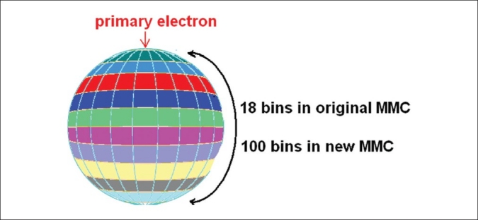
The angular range of the exited primary electron in the original MMC is 18 bins and it has been increased to 100 bins in new version of MMC, to improve the accuracy

The results of MMC are improved in the new version for homogeneous and heterogeneous phantoms. An example for a heterogeneous phantom is illustrated in Figure 11. The discrepancy between EGS4 and MMC reaches 4% (this is in contrast to the original MMC version, in which discrepancies of up to 8% were observed).

Figure 11.

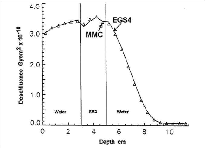
Comparison of central axis depth dose between EGS4 and MMC for 20 MeV electron beam, and 20×20 cm² field size (Ref.[14])

SUPERPOSITION MONTE CARLO

Implementation of Pre-calculated Tracks

The Superposition Monte Carlo (SMC) for electron transport is based on a simple and accurate technique, in which the code transports each electron explicitly through a microscopic ‘pre-calculated’ track.[46,47] The general purpose code, EGS4, is used for generation of the pre-calculated data. Using EGS4, electrons are transported in a large water phantom to avoid the track cut-off. The maximum allowable step size of the particle (SMAX) 24 was set to 0.05. The default setup configuration of EGS4 assigns a large step to the electron in such a medium, as the electron is far from the boundaries of the phantom; however, with decreasing maximum allowable step size, the code transports the electron in smaller steps.

In each step, various parameters such as position (x, y, z), deposited energy, and kinetic energy of the electron are saved in a file. The tracks of the secondary electrons are also saved with a different flag. The track of 3000 electrons with energies of 6 MeV and 15 MeV are simulated and saved in this way. The total energy cut-off for electron transport is ECUT=0.611 MeV, which means that the secondary electrons with kinetic energies above 100 keV are transported, while those with energies below that are deposited locally. In the final step, for generation of pre-calculated data, the stored data is post-processed. At each step, the position of the electron is converted to spherical coordinates such as step length, azimuthal angles, and polar angles (r, θ, Φ).

In SMC the electron tracks are generated in water (ρ=1 g/cm³). To transport the electrons in water-like materials (similar composition, but different density), each step is multiplied by the inverse of the density.[75] However, for other materials with a different composition and atomic number, various parameters of the electron track in water have to be modified, such as, change in scattering, stopping power ratios, collision energy loss, and bremsstrahlung production. These modifications are discussed in detail in the related article.[47]

Electron Transport in SMC

The tracks of electrons with energies of 6 or 15 MeV are picked up from the pre-calculated data and transported step by step in the voxel-based phantom. If the material of the voxel is not water, modification and scaling is done in each step. An example of an electron track for water and the same track modified for aluminum is illustrated in Figure 12. The track of the electron in aluminum is shorter because of a larger stopping power.[76] The aluminum track also has a larger lateral deflection due to the larger scattering power of the aluminum.

Figure 12.

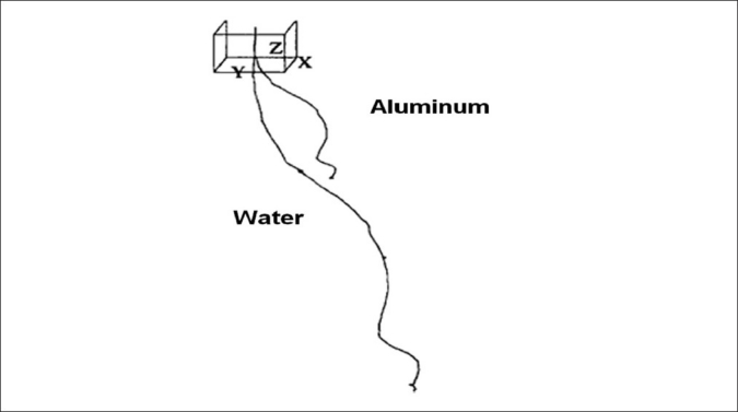
A track of the electron in water and the same track modified for aluminum. Secondary electrons are not shown. (Figure from Ref.[47])

For boundary crossing and ray tracing, in each step, if the step goes beyond the boundary of the voxel, the deposited energy is decremented by the ratio of the path length in the original voxel divided by the total length of the step. The energy deposition of the bremsstrahlung photons generated by electrons in water is ignored, as the contribution of these photons to the dose for tissue equivalent materials are negligible.[77] In the track of the primary electron, if a secondary electron is generated, the position of the primary is saved on the stack and the secondary electron is transported using the pre-generated track.

Results and Discussion of the SMC

Comparison of the SMC and EGS4 results as a reference generally shows good agreement. An example of SMC results in a water-bone phantom is illustrated in Figure 13. The results are generally in agreement to within 2–3% and the maximum difference between EGS4 and SMC is 5%. Differences of the same magnitude are observed in other homogeneous and heterogeneous cases.

Figure 13.

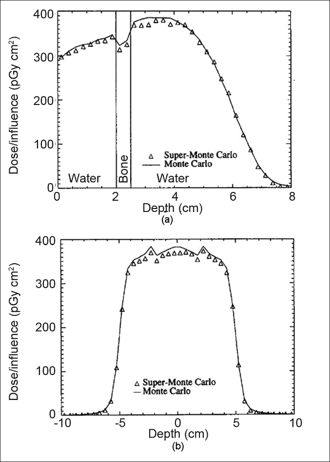
The depth dose curve of the central axis (a) and the dose profile curves of the water-bone phantom (b) for SMC and EGS4. The energy of the electrons is 15 MeV and the field size is 10×10 cm². (Figure from Ref.[47])

For the same geometry and energy cut-off, SMC runs 20 times faster than EGS4 to reach the same uncertainty. The size of the pre-calculated data for 15 MeV electrons is 15 Mb. Although the algorithm has the capability of transporting electrons with various energies, the pre-calculated electron tracks are done only for 6 and 15 MeV and no further development has been made toward including various electron energies or implementing a code using a real phase-space data (including the energy, charge, angular, and spatial distributions). Many optimizations for improvement of SMC are possible in transport parameters, such as, the number of the electron tracks, energy cut offs, and pre-processing of an electron track to join very small steps. Finally, further development of the SMC was required for its potential clinical application.[47]

VOXEL-BASED MONTE CARLO

Introduction to VMC/VMC++

Voxel based MC (VMC) was developed by Kawrakow et al. in 1996,[48] which applied some approximations and simplifications to the electron transport algorithm. One of the main approximations of VMC was the simplified treatment of multiple scattering compared to EGS4. The VMC code was very fast and produced good results, and it was improved from its original version.[78] The code was originally developed for electron transport and then extended to photon transport (XVMC).[49] In XVMX, the transport of the photon was speeded up using several variance reduction techniques. VMC simulation of the electron/photon transport was among the fastest MC codes.[8]

The VMC and XVMC have been re-developed in C++ along with other improvements in the modeling of the physical processes and variance reduction techniques, and have been introduced as the VMC++ code.[50,51] The history repetition is also implemented in the VMC and VMC++ (known as STOPS) technique, which is discussed in the following sections.

Transport Modeling in VMC

The VMC uses some approximations and modifications applicable in a typical radiation therapy problem in which the energy range is 1–30 MeV and the density of the material is in the range of 1–3 g/cm³. The transport of the electron is approximated with a simplified multiple scattering algorithm, with respect to the general purpose MC codes. With the new simplified multiple scattering model the code takes a ‘smaller number of steps’ with respect to EGS4 transport (the detail of calculation and formulations are discussed in Ref[24]).

In VMC there are also approximations in the production of secondary electrons, production of bremsstrahlung photons, and continuous energy loss of electrons. In some of these approximations, the behavior of various parameters such as the stopping power, are formulated considering the specific situation in radiation therapy (e.g., energy range 0.2–30 MeV and water-like materials). These formulations are used instead of the exact values and they are more efficient than the Table lookup, which is used in a general purpose MC code.

Reducing the number of histories with track repetition

First we assume that there are two sources of tracks with similar energy and direction. The two sources are far enough from each other, hence none of the tracks intersect with tracks from the other source, as illustrated in Figure 14. As the two beams, s₁ and s₂, do not interfere with each other, they have the same statistical uncertainty. Instead of generating new histories for s₂, the source s₁ can be reused, as it is calculated only once. Therefore, once the electron history is generated, it can be used at various positions on the surface of the phantom or patient. The only condition is that they have the same energy. In this way, computing time can be saved significantly, as parameters such as path length to discrete interactions, energies from secondary particles, and scattering angles can be removed from each other, for example, for 15 MeV electrons the points have to be more than 2 cm away from each other.[48]

Figure 14.

Two identical sources of radiation that are far from each other without any interference

Track repetition is subject to change in a heterogeneous phantom. For this purpose, the track of the electron is initially produced in water. The characteristics of the electron track such as deposited energy, path length, scattering angle, and electron energy are saved on the fly. The path length and scattering angles are then adjusted according to the material and the density of the medium. The difference between the track repetition in SMC and VMC is that in SMC the entire track is already available in the pre-calculated data, while in VMC the track is generated on the fly and it is repeated for various positions. Each of these techniques has its own advantages, which are discussed later in the text.

Results of VMC

The calculations using the original version of VMC were done with a 0.2 MeV energy cut-off for electrons and 0.01 MeV cut off for photons. The results were compared with the EGS4 that served as a reference. As an example of track repetition, for a 10×10 cm² field and one million histories, 50000 electrons were generated and repeated 20 times in 20 different locations. Figure 15a illustrates the results of VMC for monoenergetic electrons in comparison with EGS4.

Figure 15.

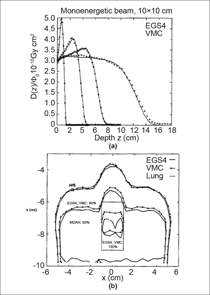
(a) Depth dose calculation of VMC for 2, 9, 30 MeV electron beams with EGS4 code. The uncertainties in calculations are less than 1%. (b) Comparison of isodose lines of VMC and EGS4 in the water phantom with a lung slab, density=0.26 g/cm³. (Figures from Ref.[48])

In the discussion on the results for monoenergetic electrons, about the big discrepancies, it is mentioned that:[48] “When performing dose calculation for beams used in radiation therapy, these deviations will be removed in homogeneous phantoms due to the fact that different energy spectra are required for VMC and EGS4 in order to describe measured dose distribution.”

The VMC code performs well in various heterogeneous cases such as water-lung and -air phantoms, as illustrated in Figure 15b. There is generally a good agreement between the two codes and deviations are due to approximations in the cross sections and in the multiple scattering method. The computational speed is increased by a factor of 35 with respect to EGS4. In the first article on VMC,[48] the linear accelerator is modeled in a very simple manner and good agreement between the VMC results and measurements of dose distribution for a 16 MeV electron beam is found. As no pre-calculated data is needed for VMC dose calculation, the amount of needed memory is very small and depends on the resolution of the 3D phantom, for example, for a 128×128×50 matrix representing a CT phantom, 16 Mb of RAM is required. In the follow-up articles VMC has been improved and licensed to a number of manufactuturers.[35]

VMC++ and STOPS

VMC++ was developed by Kawrakow in 2000, with the C++ programming language, using an object-oriented design.[50] The code includes all VMC/XVMC variance reduction techniques, but incorporates several improvements in the modeling of the underlying physical processes:

1. Use of the exact multiple elastic scattering theory employed in EGSnrc[51]

2. Use of STOPS technique instead of history repetition

3. Refinements in the simulation of various scattering processes such as corrections for Compton scattering

VMC++ is used as the dose calculation tool for the first commercial electron MC algorithm from Nucletron and is being incorporated into the Masterplan (Nucletron) and Eclipse (Varian) treatment planning systems, for photon beam dose calculations.[79]

Simultaneous transport of particle sets (STOPS)

Track repetition in VMC introduces systematic uncertainties and limits the applicability of the algorithm to low z materials discussed in the previous section. VMC++ uses a new technique for track repetition that removes the systematic uncertainties. In the STOPS technique, a group of the particles are transported at the ‘same time’ from various positions. The particles have the same energy, but different positions and directions. The interaction type of the particle is sampled separately based on the interaction probabilities of each medium. For all particles, in each group, several material independent parameters are sampled once, such as interpolation indices, azimuthal scattering angles, and distances to discrete interactions.

An example of VMC++ in comparison with EGSnrc is illustrated in Figure 16. 20 MeV electrons inside a lead medium with a 10×10 cm² field size have been simulated. As one sees there is an excellent agreement between the results of the code, with errors up to 1%.

Figure 16.

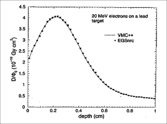
Comparison of VMC++ code with EGSnrc general purpose code for 20 MeV electrons. The material is lead and field size is 10×10 cm² (Figure from Ref[27])

In discussion of the STOPS technique there is a very important hint about track repetition and its effect on statistical uncertainties, which is discussed here.

The efficiency of the Monte Carlo code is defined as

in which T is the computing time and σ is the statistical uncertainty. Each particle group in STOPS can have various numbers of particles; however, after a certain number of repetitions, the tracks of the particles are correlated, although the efficiency is not improved.

An example of the effect of track repetition on efficiency, denoted by Kawrakow,[27] is illustrated in Figure 17. The Figure shows the relative efficiency of the VMC++ code for 20 MeV electrons and 10×10 cm² field size in a phantom of four randomly distributed materials (lung, carbon, water, aluminum). The size of the voxels is 5 mm in each direction and the efficiency is plotted versus the number of repetitions.

Figure 17.

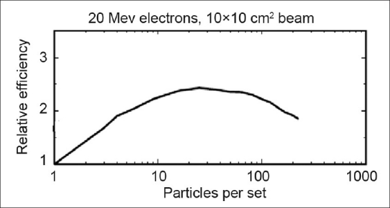
The relative efficiency of the VMC++ code as a function of the number of track repetitions (particle per set). (Figure from Ref.[27])

As one can see, the change in the efficiency versus the number of repetitions is initially increased, reaches a maximum, and then decreases for a large number of repetitions. The initial rise is because of the time that is saved by STOPS (up to 20 to 30 repetitions) and then the efficiency decreases, as the uncertainty reaches a limit and the time still increases in Eq. 3.

VMC++ is benchmarked with various clinical situations and it is also evaluated and implemented in photon–electron transport by other groups.[65,79–85] The results of the code agree with EGSnrc in the sub-percent level, while the code itself runs 50 times faster than the EGS4, for electron transport.

CONCLUSION

In the past decade, many fast MC codes have been developed for application in medical physics.[86–90] Considering the detailed discussion of MMC, SMC, and VMC, fast MC codes take two general approaches to accelerate dose calculations. In one approach, the transport parameters and algorithms of the particles are formulated in an efficient form, considering the specific conditions that one encounters in clinical situations. These specific conditions include a relatively smaller energy range, that is, < 30 MeV, and low-Z materials with densities up to 3 g/cm³. This general feature is employed in ‘from scratch’ MC codes such as the VMC,[48] Dose Planning Method (DPM),[52] and MCDOSE[53] code suites. DPM[91–96] and MCDOSE[96–99] are integrated into the treatment planning systems and they are currently being used for a variety of electron–photon beam treatment planning studies.

In another approach fast MC codes use pre-generated data for particle transport. An important advantage of developing a fast MC code using pre-generated data is that the physics can be handled accurately by a general purpose code and after generation of the pre-calculated tracks, one technically needs only simple methods to apply the tracks to the problem of interest. In this manner, various particles can be simulated with the same transport algorithm. The dramatic evolution in computer speed and large available memory has enabled several groups to develop their own fast MC codes based on pre-calculated data for application in radiation therapy.[100–103] Most of the codes use the EGS4/EGSnrc code for generation of pre-calculated data and they need a relatively large amount of memory to load the data.

BIOGRAPHY

Keyvan Jabbari received B.S. degree in physics from Isfahan University of Technology, Isfahan, IRAN in 1999, M.S. degree in medical radiation engineering from Amir Kabir University, Tehran in 2002, M.S. degree in medical physics from University of Manitoba , Winnipeg, Canada, in 2004. Then he got Ph.D. of Medical Physics from McGill University, Montreal, Canada in 2008.

Since then, he is assistant professor in Department of Medical Physics and Medical Engineering, School of Medicine, Isfahan University of Medical Sciences. He is also clinical medical physicist in Milad Hospital and Seyed-o-Shohada cancer center.

His research interest is fast Monte Carlo in treatment planning, dose calculation and plan optimization.

REFERENCES

- 1.Goitein M, Busse J. Immobilization error: Some theoretical considerations. Radiology. 1975;117:407–12. doi: 10.1148/117.2.407. [DOI] [PubMed] [Google Scholar]
- 2.Ito A. In: In Monte Carlo Transport of Electrons and Photons. Nelson W. R, Jenkins T. M, Rindi A, Nahum A. E, Rogers D. W. O, editors. New York: Plenum Press; 1988. pp. 573–98. [Google Scholar]
- 3.Nahum A. E. In: In Monte Carlo Transport of Electrons and Photons. Nelson W. R, Jenkins T. M, Rindi A, Nahum A. E, Rogers D. W, editors. New York: Plenum Press; 1988. pp. 3–20. [Google Scholar]
- 4.Berger M. J. In: In Methods in Computational Physics. Fernbach S, Alder B, Rothenberg M, editors. Vol. 1. New York: Academic; 1963. [Google Scholar]
- 5.Rogers D. W, Bielajew A. F. The Dosimetry of Ionization Radiation. Vol. 3. New York: Academic Press; 1990. Monte Carlo techniques of electron and photon transport for radiation dosimetry. Chapter 5. [Google Scholar]
- 6.Andreo P. Monte Carlo techniques in medical radiation physics. Phys Med Biol. 1991;36:861–920. doi: 10.1088/0031-9155/36/7/001. [DOI] [PubMed] [Google Scholar]
- 7.Raeside D. E. Monte Carlo principles and applications. Phys Med Biol. 1976;21:181–97. doi: 10.1088/0031-9155/21/2/001. [DOI] [PubMed] [Google Scholar]
- 8.Chetty I, Curran B, Cygler J, DeMarco J, Faddegon B, Liu H, et al. Guidance report on clinical implementation of the Monte Carlo method in external beam radiation therapy treatment planning: Report of the AAPM Task Group No. 105. Med Phys. 2007;34:4818–53. doi: 10.1118/1.2795842. [DOI] [PubMed] [Google Scholar]
- 9.Verhaegen F, Seuntjens J. Monte Carlo modelling of external radiotherapy photon beams. Phys Med Biol. 2003;48:R107–64. doi: 10.1088/0031-9155/48/21/r01. [DOI] [PubMed] [Google Scholar]
- 10.Fippel M, Soukup M. A Monte Carlo dose calculation algorithm for proton therapy. Med Phys. 2004;31:2263–73. doi: 10.1118/1.1769631. [DOI] [PubMed] [Google Scholar]
- 11.Ma C. M, Jiang S. B. Monte Carlo modelling of electron beams from medical accelerators. Phys Med Biol. 1999;44:R157–89. doi: 10.1088/0031-9155/44/12/201. [DOI] [PubMed] [Google Scholar]
- 12.Doucet R, Olivares M, DeBlois F, Podgorsak E. B, Kawrakow I, Seuntjens J. Comparison of measured and Monte Carlo calculated dose distributions in inhomogeneous phantoms in clinical electron beams. Phys Med Biol. 2003;48:2339–54. doi: 10.1088/0031-9155/48/15/307. [DOI] [PubMed] [Google Scholar]
- 13.Wang L, Chui C. S, Lovelock M. A patient-specific Monte Carlo dose-calculation method for photon beams. Med Phys. 1998;25:867–78. doi: 10.1118/1.598262. [DOI] [PubMed] [Google Scholar]
- 14.Pacilio M, Aragno D, Rauco R, D’Onofrio S, Pressello M. C, Bianciardi L, et al. Monte Carlo dose calculations using MCNP4C and EGSnrc / BEAMnrc codes to study the energy dependence of the radiochromic film response to beta-emitting sources. Phys Med Biol. 2007;52:3931–48. doi: 10.1088/0031-9155/52/13/018. [DOI] [PubMed] [Google Scholar]
- 15.Berger M, Seltzer S. Oak Ridge National Laboratory: Oak Ridge, TN; 1973. ETRAN Monte Carlo code system for electron and photon transport through extended media, Radiation Shielding Information Center (RSIC) Report CCC-107. [Google Scholar]
- 16.Sheikh-Bagheri D, Rogers D. W. Sensitivity of megavoltage photon beam Monte Carlo simulations to electron beam and other parameters. Med Phys. 2002;29:379–90. doi: 10.1118/1.1446109. [DOI] [PubMed] [Google Scholar]
- 17.Ding G. X. Energy spectra, angular spread, fluence profiles and dose distributions of 6 and 18 MV photon beams: Results of Monte Carlo simulations for a Varian 2100EX accelerator. Phys Med Biol. 2002;47:1025–46. doi: 10.1088/0031-9155/47/7/303. [DOI] [PubMed] [Google Scholar]
- 18.Tyagi N, Moran J. M, Litzenberg D. W, Bielajew A. F, Fraass B. A, Chetty I. J. Experimental verification of a Monte Carlo-based MLC simulation model for IMRT dose calculation. Med Phys. 2007;34:651–63. doi: 10.1118/1.2428405. [DOI] [PubMed] [Google Scholar]
- 19.Podgorsak E. B. New York: Plenum Press; 2005. Radiation Physics for Medical Physicists. [Google Scholar]
- 20.Chetty I. J. Monte Carlo treatment planning: The influence of ‘variance reduction’ techniques (ECUT, PCUT, ESTEP) on the accuracy and speed of dose calculations. Med Phys. 2005;32:2018. (abstract) [Google Scholar]
- 21.Rogers D. W, Faddegon B. A, Ding G. X, Ma C. M, We J, Mackie T. R. BEAM: A Monte Carlo code to simulate radiotherapy treatment units. Med Phys. 1995;22:503–24. doi: 10.1118/1.597552. [DOI] [PubMed] [Google Scholar]
- 22.Kawrakow I, Rogers D. W, Walters B. R. Large efficiency improvements in BEAMnrc using directional bremsstrahlung splitting. Med Phys. 2004;31:2883–98. doi: 10.1118/1.1788912. [DOI] [PubMed] [Google Scholar]
- 23.Rogers D. W, Bielajew A. F. In: In Monte Carlo Transport of Electrons and Photons. Nelson W. R, Jenkins T. M, Rindi A, Nahum A. E, Rogers D. W, editors. New York: Plenum Press; 1988. pp. 407–19. [Google Scholar]
- 24.Nelson W. R, Hirayama H., Rogers D. W. The EGS4 Code System. SLAC Report No. SLAC-265. 1985 [Google Scholar]
- 25.Kawrakow I, Rogers D. W. The EGSnrc code system: Monte Carlo simulation of electron and photon transport. NRC, Report PIRS–701. 2000 [Google Scholar]
- 26.Briesmeister J. F. MCNP-A general Monte Carlo N-particle transport code, Version 4C. Report LA-13709-M, Los Alamos National Laboratory,NM. 2000 [Google Scholar]
- 27.Agostinelli S, Allison J, Amako K, Apostolakis J, Araujo H, Arce P, et al. GEANT4-A simulation toolkit. Nucl Instrum Methods Phys Res A. 2003;506:250–303. [Google Scholar]
- 28.Rogers D. W, Walters B, Kawrakow I. BEAMnrc Users Manual. NRC Report PIRS 509(a)revH. 2004 [Google Scholar]
- 29.Walters B. R, Kawrakow I, Rogers D. W. DOSXYZnrc Users Manual. NRC Report PIRS 794 (rev B) 2005 [Google Scholar]
- 30.Wang L. L, Rogers D. W. Calculation of the replacement correction factors for ion chambers in megavoltage beams by Monte Carlo simulation. Med Phys. 2008;35:1747–55. doi: 10.1118/1.2898139. [DOI] [PubMed] [Google Scholar]
- 31.Joshi C. P, Darko J, Vidyasagar P. B, Schreiner L. J. Investigation of an efficient source design for Cobalt-60-based tomotherapy using EGSnrc Monte Carlo simulations. Phys Med Biol. 2008;53:575–92. doi: 10.1088/0031-9155/53/3/005. [DOI] [PubMed] [Google Scholar]
- 32.La Russa D. J, McEwen M, Rogers D. W. An experimental and computational investigation of the standard temperature-pressure correction factor for ion chambers in kilovoltage x rays. Med Phys. 2007;34:4690–9. doi: 10.1118/1.2799580. [DOI] [PubMed] [Google Scholar]
- 33.Toye W. C, Das K. R, Todd S. P, Kenny M. B, Franich R. D, Johnston P. N. An experimental MOSFET approach to characterize (192)Ir HDR source anisotropy. Phys Med Biol. 2007;52:5329–39. doi: 10.1088/0031-9155/52/17/015. [DOI] [PubMed] [Google Scholar]
- 34.Fogliata A, Vanetti E, Albers D, Brink C, Clivio A, Knöös T. On the dosimetric behaviour of photon dose calculation algorithms in the presence of simple geometric heterogeneities: comparison with Monte Carlo calculations. Phys Med Biol. 2007;52:1363–85. doi: 10.1088/0031-9155/52/5/011. [DOI] [PubMed] [Google Scholar]
- 35.Strigari L, Menghi E, D’Andrea M, Benassi M. Monte Carlo dose voxel kernel calculations of beta-emitting and Auger-emitting radionuclides for internal dosimetry: A comparison between EGSnrcMP and EGS4. Med Phys. 2006;33:3383–9. doi: 10.1118/1.2266255. [DOI] [PubMed] [Google Scholar]
- 36.Abdel-Rahman W, Seuntjens J. P, Verhaegen F, Podgorsak E. B. Radiation induced currents in parallel plate ionization chambers: Measurement and Monte Carlo simulation for megavoltage photon and electron beams. Med Phys. 2006;33:3094–104. doi: 10.1118/1.2208917. [DOI] [PubMed] [Google Scholar]
- 37.Verhaegen F. Evaluation of the EGSnrc Monte Carlo code for interface dosimetry near high-Z media exposed to kilovolt and 60Co photons. Phys Med Biol. 2002;47:1691–705. doi: 10.1088/0031-9155/47/10/306. [DOI] [PubMed] [Google Scholar]
- 38.Holmes M. A, Mackie T. R, Sohn W, Reckwerdt P. J, Kinsella T. J, Bielajew A. F, et al. The application of correlated sampling to the computation of electron beam dose distributions in heterogeneous phantoms using the Monte Carlo method. Phys Med Biol. 1993;38:675–88. doi: 10.1088/0031-9155/38/6/003. [DOI] [PubMed] [Google Scholar]
- 39.Court L. E, Jahnke L, Chin D, Song J, Cormack R, Zygmanski P, et al. Dynamic IMRT treatments of sinus region tumors: Comparison of Monte Carlo calculations with treatment planning system calculations and ion chamber measurements. Technol Cancer Res Treat. 2006;5:489–95. doi: 10.1177/153303460600500505. [DOI] [PubMed] [Google Scholar]
- 40.Cho S. H, Vassiliev O. N, Lee S, Liu H. H, Ibbott G. S, Mohan R. Reference photon dosimetry data and reference phase space data for the 6 MV photon beam from varian clinac 2100 series linear accelerators. Med Phys. 2005;32:137–48. doi: 10.1118/1.1829172. [DOI] [PubMed] [Google Scholar]
- 41.Kawrakow I, Walters B. Efficient photon beam dose calculations using DOSXYZnrc with BEAMnrc. Med Phys. 2006;33:3046–56. doi: 10.1118/1.2219778. [DOI] [PubMed] [Google Scholar]
- 42.Furhang E. E, Chui C. S, Kolbert K. S, Larson S. M, Sgouros G. Implementation of a Monte Carlo dosimetry method for patient specific internal emitter therapy. Med Phys. 1997;24:1163–72. doi: 10.1118/1.598018. [DOI] [PubMed] [Google Scholar]
- 43.Ma C.-M, Mok E, Kapur A, Pawlicki T, Findley D, Brain S, et al. Clinical implementation of a Monte Carlo treatment planning system. Med Phys. 1999;26:2133–43. doi: 10.1118/1.598729. [DOI] [PubMed] [Google Scholar]
- 44.Neuenschwander H, Born E. J. A Macro Monte Carlo method for electron beam dose calculations. Phys Med Biol. 1992;37:107–25. [Google Scholar]
- 45.Neuenschwander H, Mackie T. R, Reckwerdt P. J. MMC— A highperformance Monte Carlo code for electron beam treatment planning. Phys Med Biol. 1995;40:543–74. doi: 10.1088/0031-9155/40/4/005. [DOI] [PubMed] [Google Scholar]
- 46.Keall P. J, Hoban P. W. Super-Monte Carlo: A 3D electron beam dose calculation algorithm. Med Phys. 1996;23:2023–34. doi: 10.1118/1.597842. [DOI] [PubMed] [Google Scholar]
- 47.Keall P. J, Hoban P. W. Superposition dose calculation incorporating Monte Carlo generated electron track kernels. Med Phys. 1996;23:479–85. doi: 10.1118/1.597679. [DOI] [PubMed] [Google Scholar]
- 48.Kawrakow I, Fippel M, Friedrich K. 3D Electron Dose Calculation using a Voxel based Monte Carlo Algorithm. Med Phys. 1996;23:445–57. doi: 10.1118/1.597673. [DOI] [PubMed] [Google Scholar]
- 49.Kawrakow I, Fippel M. Investigation of variance reduction techniques for Monte Carlo photon dose calculation using XVMC. Phys Med Biol. 2000;45:2163–84. doi: 10.1088/0031-9155/45/8/308. [DOI] [PubMed] [Google Scholar]
- 50.Kawrakow I, Fippel M. in Proceedingsof the 22nd Annual International Conference of the IEEE (Engineering in Medicine and Biology Society) Piscataway, NJ: 2000. VMC++, a MC algorithm optimized for electron and photon beam dose calculations for RTP. [Google Scholar]
- 51.Kawrakow I. VMC++, electron and photon Monte Carlo calculations optimized for Radiation Treatment Planning, Advanced Monte Carlo for Radiation Physics, Particle Transport Simulation and Applications. In: Kling A, Barao F, Nakagawa M, Távora L, Vaz P, editors. Proceedings of the Monte Carlo 2000 Meeting Lisbon. Berlin: Springer; 2001. pp. 229–36. [Google Scholar]
- 52.Sempau J, Wilderman S. J, Bielajew A. F. DPM, a fast, accurate Monte Carlo code optimized for photon and electron radiotherapy treatment planning dose calculations. Phys Med Biol. 2000;45:2263–91. doi: 10.1088/0031-9155/45/8/315. [DOI] [PubMed] [Google Scholar]
- 53.Ma C, Li J. S, Pawlicki T, Jiang S. B, Deng J, Lee M. C, et al. MCDOSE- A Monte Carlo dose calculation tool for radiation therapy treatment planning. Phys Med Biol. 2002;47:1671–89. doi: 10.1088/0031-9155/47/10/305. [DOI] [PubMed] [Google Scholar]
- 54.Rosu M, Balter J. M, Chetty I. J, Kessler M. L, Mc Shan D. L, Balter P, et al. How extensive of a 4D dataset is needed to estimate cumulative dose distribution plan evaluation metrics in conformal lung therapy? Med Phys. 2007;34:233–45. doi: 10.1118/1.2400624. [DOI] [PubMed] [Google Scholar]
- 55.Keall P. J, Siebers J. V, Joshi S, Mohan R. Monte Carlo as a fourdimensional radiotherapy treatment-planning tool to account for respiratory motion. Phys Med Biol. 2004;49:3639–48. doi: 10.1088/0031-9155/49/16/011. [DOI] [PubMed] [Google Scholar]
- 56.Jeraj R, Keall P. The effect of statistical uncertainty on inverse treatment planning based on Monte Carlo dose calculation. Phys Med Biol. 2002;45:3601–13. doi: 10.1088/0031-9155/45/12/307. [DOI] [PubMed] [Google Scholar]
- 57.Jeraj R, Keall P. J. Monte Carlo-based inverse treatment planning. Phys Med Biol. 1999;44:1885–96. doi: 10.1088/0031-9155/44/8/303. [DOI] [PubMed] [Google Scholar]
- 58.Chetty I. J, Charland P. M, Tyagi N, Mc Shan D. L, Fraass B. A, Bielajew A. F. Photon beam relative dose validation of the DPM Monte Carlo code in lung-equivalent media. Med Phys. 2003;30:563–73. doi: 10.1118/1.1555671. [DOI] [PubMed] [Google Scholar]
- 59.Chetty I. J, Moran J. M, Nurushev T. S, McShan D. L, Fraass B. A, Wilderman S. J, et al. Experimental validation of the DPM Monte Carlo code using minimally scattered electron beams in heterogeneous media. Phys Med Biol. 2002;47:1837–51. doi: 10.1088/0031-9155/47/11/301. [DOI] [PubMed] [Google Scholar]
- 60.Fippel M, Kawrakow I, Friedrich K. Electron beam dose calculations with the VMC algorithm and the verification data of the NCI working group. Phys Med Biol. 1997;42:501–20. doi: 10.1088/0031-9155/42/3/005. [DOI] [PubMed] [Google Scholar]
- 61.Popple R. A, Weinberg R, Antolak J. A, Ye S. J, Pareek P. N, Duan J, et al. A Comprehensive evaluation of a commercial macro Monte Carlo electron dose calculation implementation using a standard verification data set. Med Phys. 2006;33:1540–551. doi: 10.1118/1.2198328. [DOI] [PubMed] [Google Scholar]
- 62.Ding G. X, Duggan D. M, Coffey C. W, Shokrani P, Cygler J. E. First macro Monte Carlo based commercial dose calculation module for electron beam treatment planning-new issues for clinical consideration. Phys Med Biol. 2006;51:2781–99. doi: 10.1088/0031-9155/51/11/007. [DOI] [PubMed] [Google Scholar]
- 63.Gardner J, Siebers J, Kawrakow I. Dose calculation validation of VMC++ for photon beams. Med Phys. 2007;34:1809–18. doi: 10.1118/1.2714473. [DOI] [PubMed] [Google Scholar]
- 64.Hasenbalg F., Fix M. K., Born E. J., Mini R., Kawrakow I. VMC++ versus BEAMnrc: A comparison of simulated linear accelerator heads for photon beams. Med Phys. 2008;35:1521. doi: 10.1118/1.2885372. [DOI] [PubMed] [Google Scholar]
- 65.Siebers J. V., Kawrakow I., Ramakrishnan V. Performance of a hybrid MC dose algorithm for IMRT optimization dose evaluation. Med Phys. 2007;34:2853. doi: 10.1118/1.2745236. [DOI] [PubMed] [Google Scholar]
- 66.Kawrakow I. Improved modeling of multiple scattering in the Voxel Monte Carlo model. Med Phys. 1997;24:505–17. doi: 10.1118/1.597933. [DOI] [PubMed] [Google Scholar]
- 67.Ma C., Li J., Deng J., Fan J. Investigation of Fast Monte Carlo Dose Calculation for CyberKnife SRS / SRT Treatment Planning. Med Phys. 2007;34:2589–90. [Google Scholar]
- 68.Hogstrom K. R. Evaluation of electron pencil beam dose calculation. Med Phys. 1985;12:554. [Google Scholar]
- 69.Shiu A. S., Hogstrom K. R. Pencil-beam redefinition algorithm for electron dosedistributions. Med Phys. 1991;18:7–18. doi: 10.1118/1.596697. [DOI] [PubMed] [Google Scholar]
- 70.Cygler J., Battista J. J., Scrimger J. W., Mah E., Antolak J. Electron dose distributions in experimental phantoms: A comparison with 2D pencil beam calculations. Phys Med Biol. 1987;32:1073–86. doi: 10.1088/0031-9155/32/9/001. [DOI] [PubMed] [Google Scholar]
- 71.Lax I. Inhomogeneity corrections in electron beam dose planning. Limitations with the semi-infinite slab approximation. Phys Med Biol. 1986;31:879–92. doi: 10.1088/0031-9155/31/8/006. [DOI] [PubMed] [Google Scholar]
- 72.Cris C., Born E., Mini R., Neuenschwander H., Volken W. A scaling method for multiple source models, in Proceedings of the 13th ICCR. In: Bortfeld T., Schlegel W., editors. Heidelberg: Springer-Verlag; 2000. pp. 411–3. [Google Scholar]
- 73.Pemler P., Besserer J., Schneider U., Neuenschwander H. Evaluation of a commercial electron treatment planning system based on Monte Carlo techniques (eMC) Med Phys. 2006;16:313–29. doi: 10.1078/0939-3889-00330. [DOI] [PubMed] [Google Scholar]
- 74.Siddon R. L. Prism representation: A 3D ray-tracing algorithm for radiotherapy applications. Phys Med Biol. 1985;30:817–24. doi: 10.1088/0031-9155/30/8/005. [DOI] [PubMed] [Google Scholar]
- 75.Connor J. E. The variation of scattered X-rays with density in an irradiated body. Phys Med Biol. 1957;1:352–69. doi: 10.1088/0031-9155/1/4/305. [DOI] [PubMed] [Google Scholar]
- 76.Report of the Task Group on Reference Man. Vol. 23. Pergamon, New York: 1974. International Commission on Radiological Protection. [Google Scholar]
- 77.Rustgi S. N., Rodgers J. E. Analysis of the bremsstrahlung component in 6-18 MeV electron beams. Med Phys. 1987;14:884–8. doi: 10.1118/1.596018. [DOI] [PubMed] [Google Scholar]
- 78.Kawrakow I., Bielajew A. F. On the representation of electron multiple elastic-scattering distributions for Monte Carlo calculations. Nucl Instrum Methods Phys Res B. 1998;134:325–36. [Google Scholar]
- 79.Scherf C., Scherer J., Bogner L. Verification and application of the Voxel-based Monte Carlo (VMC++) electron dose module of oncentratrade mark MasterPlan. Strahlenther Onkol. 2007;183:81–8. doi: 10.1007/s00066-007-1602-8. [DOI] [PubMed] [Google Scholar]
- 80.Fogliata A., Nicolini G., Vanetti E., Clivio A., Winkler P., Cozzi. L. The impact of photon dose calculation algorithms on expected dose distributions in lungs under different respiratory phases. Phys Med Biol. 2008;53:2395–90. doi: 10.1088/0031-9155/53/9/011. [DOI] [PubMed] [Google Scholar]
- 81.Vatanen T., Traneus E., Lahtinen T. Dosimetric verification of a Monte Carlo electron beam model for an add-on eMLC. Phys Med Biol. 2008;53:391–404. doi: 10.1088/0031-9155/53/2/007. [DOI] [PubMed] [Google Scholar]
- 82.Gardner J. K., Siebers J. V., Kawrakow I. Comparison of two methods to compute the absorbed dose to water for photon beams. Phys Med Biol. 2007;52:439–47. doi: 10.1088/0031-9155/52/19/N02. [DOI] [PubMed] [Google Scholar]
- 83.Hasenbalg F., Neuenschwander H., Mini R., Born E. J., et al. Collapsed cone convolution and analytical anisotropic algorithm dose calculations compared to VMC++ Monte Carlo simulations in clinical cases. Phys Med Biol. 2007;52:3679–91. doi: 10.1088/0031-9155/52/13/002. [DOI] [PubMed] [Google Scholar]
- 84.Lindsay P. E., Naqa I. El, Hope A. J., Vicic M., Cui J., Bradley J. D., et al. Retrospective monte carlo dose calculations with limited beam weight information. Med Phys. 2007;34:334–46. doi: 10.1118/1.2400826. [DOI] [PubMed] [Google Scholar]
- 85.Zakarian C., Deasy J. O. Beamlet dose distribution compression and reconstruction using wavelets for intensity modulated treatment planning. Med Phys. 2004;31:368–75. doi: 10.1118/1.1636560. [DOI] [PubMed] [Google Scholar]
- 86.Eklund K., Ahnesjö A. Fast modelling of spectra and stoppingpower ratios using differentiated fluence pencil kernels. Phys Med Biol. 2008;53:4231–47. doi: 10.1088/0031-9155/53/16/002. [DOI] [PubMed] [Google Scholar]
- 87.Oliver M., Staruch R., Gladwish A., Craig J., Chen J., Wong E. Monte Carlo dose calculation of segmental IMRT delivery to a moving phantom using dynamic MLC and gating log files. Phys Med Biol. 2008;53:187–96. doi: 10.1088/0031-9155/53/10/N03. [DOI] [PubMed] [Google Scholar]
- 88.Fippel M. Fast Monte Carlo dose calculation for photon beams based on the VMC electron algorithm. Med Phys. 1999;26:1466–75. doi: 10.1118/1.598676. [DOI] [PubMed] [Google Scholar]
- 89.Li J. S., Shanine B., Fourkal E., Ma. C.-M. A particle track-repeating algorithm for proton beam dose calculation. Phys Med Biol. 2005;50:1001–10. doi: 10.1088/0031-9155/50/5/022. [DOI] [PubMed] [Google Scholar]
- 90.Semenenko V. A., Stewart R. D. Fast Monte Carlo simulation of DNA damage formed by electrons and light ions. Phys Med Biol. 2005;51:1693–706. doi: 10.1088/0031-9155/51/7/004. [DOI] [PubMed] [Google Scholar]
- 91.Chetty I. J., Tyagi N., Rosu M., Charland P. M., McShan D. L., Haken R. K. Ten, et al. Nuclear Mathematical and Computational Sciences: A Century in Review, A Century Anew, Gatlinburg, TN. Vol. 119. LaGrange Park: American Nuclear Society; 2003. Clinical implementation, validation and use of the DPM Monte Carlo code for radiotherapy treatment planning; pp. 1–17. [Google Scholar]
- 92.Tyagi N., Bose A., Chetty I. J. Implementation of the DPM Monte Carlo Code on a parallel architecture for treatment planning applications. Med Phys. 2004;31:2271–5. doi: 10.1118/1.1786691. [DOI] [PubMed] [Google Scholar]
- 93.Chetty I. J., Charland P. M., Tyagi N., McShan D. L., Fraass B., Bielajew A. F. Experimental validation of the DPM Monte Carlo code for photon beam dose calculations in inhomogeneous media. Med Phys. 2002;29:1351. (abstract) [Google Scholar]
- 94.Weng X., Yan Y., Shu H., Wang J., Jiang S. B., Luo L. A vectorized Monte Carlo code for radiotherapy treatment planning dose calculation. Phys Med Biol. 2003;48:N111–20. doi: 10.1088/0031-9155/48/7/401. [DOI] [PubMed] [Google Scholar]
- 95.Lee T. K., Sandisonm G. A. The energy-dependent electron loss model: Backscattering and application to heterogeneous slab media. Phys Med Biol. 2003;48:259–73. doi: 10.1088/0031-9155/48/2/308. [DOI] [PubMed] [Google Scholar]
- 96.Rosu M., Chetty I. J., Tatro D. S., Ten Haken R. K. The impact of breathing motion versus heterogeneity effects in lung cancer treatment planning. Med Phys. 2007;34:1462–73. doi: 10.1118/1.2713427. [DOI] [PubMed] [Google Scholar]
- 97.Ma C.M-, Li J. S., Pawlicki T., Jiang S. B., Deng J. MCDOSE—A Monte Carlo dose calculation tool for radiation therapy treatment planning, in Proceedings of the 13th ICCR. In: Bortfeld T., Schlegel W., editors. Heidelberg: Springer-Verlag; 2000. pp. 411–3. [Google Scholar]
- 98.Blomquist M, Li J., Ma C. M., Zackrisson B., Karlsson M. Comparison between a conventional treatment energy and 50 MV photons for the treatment of lung tumors. Phys Med Biol. 2002;47:889–97. [PubMed] [Google Scholar]
- 99.Lee M. C., Jiang S. B., Ma. C. M. Monte Carlo and experimental investigations of multileaf collimated electron beams for modulated electron radiation therapy. Med Phys. 2000;27:2708–18. doi: 10.1118/1.1328082. [DOI] [PubMed] [Google Scholar]
- 100.Sheu R, Chui C., LoSasso T., Lim S., Kirov A. Accurate and Efficient Monte Carlo Dose Calculation for Electron Beams. Med Phys. 2006;33:2067. [Google Scholar]
- 101.Stathakis S., Li J., Ma. C. M. Monte Carlo determination of radiation-induced cancer risks for prostate patients undergoing intensity- modulated radiation therapy. J Appl Clin Med Phys. 2007;8:2685. doi: 10.1120/jacmp.v8i4.2685. [DOI] [PMC free article] [PubMed] [Google Scholar]
- 102.Flampouri S., Jiang S. B., Sharp G. C., Wolfgang J., Patel A. A., Choi N. C. Estimation of the delivered patient dose in lung IMRT treatment based on deformable registration of 4D-CT data and Monte Carlo simulations. Phys Med Biol. 2006;51:2763–79. doi: 10.1088/0031-9155/51/11/006. [DOI] [PubMed] [Google Scholar]
- 103.Yang J., Li J. S., Qin L., Xiong W., Ma C. M. Modelling of electron contamination in clinical photon beams for Monte Carlo dose calculation. Phys Med Biol. 2004;49:2657–73. doi: 10.1088/0031-9155/49/12/013. [DOI] [PubMed] [Google Scholar]